Anomaly Detection Using Predictive Convolutional Long Short-Term Memory Units

Rochester Institute of Technology

RIT Scholar Works

Theses Thesis/Dissertation Collections

11-2016

Anomaly Detection Using Predictive

Convolutional Long Short-Term Memory Units

[email protected]

Follow this and additional works at:http://scholarworks.rit.edu/theses

This Thesis is brought to you for free and open access by the Thesis/Dissertation Collections at RIT Scholar Works. It has been accepted for inclusion in Theses by an authorized administrator of RIT Scholar Works. For more information, please [email protected].

Recommended Citation

Anomaly Detection Using Predictive Convolutional Long

Short-Term Memory Units

by

Jefferson Ryan Medel

A Thesis Submitted in Partial Fulfillment of the Requirements for the Degree of Master of Science in Computer Engineering

Supervised by

Dr. Andreas Savakis

Department of Computer Engineering Kate Gleason College of Engineering

Rochester Institute of Technology Rochester, NY

November 2016

Approved By:

_______________________________________________________________________________

Dr. Andreas Savakis

Primary Advisor – R.I.T. Dept. of Computer Engineering

_______________________________________________________________________________

Dr. Andres Kwasinski

Secondary Advisor – R.I.T. Dept. of Computer Engineering

_______________________________________________________________________________

Dr. Roy Melton

Dedication

I would like to dedicate this thesis to my loving parents, Ric and Juliet Medel, and sister,

Acknowledgements

I would like to thank my advisor Dr. Andreas Savakis for his assistance and work guiding

me through the development of this thesis, and my committee members Dr. Andres

Kwasinski and Dr. Roy Melton for their time. I also want to thank my colleagues in the

Computer Vision Lab, Peter Muller, Dan Chianucci, and Breton Minnehan, for their

Abstract

Automating the segmentation of anomalous activities within long video sequences

is complicated by the ambiguity of how such events are defined. This thesis approaches

the problem by learning generative models with which meaningful sequences can be

identified in videos using limited supervision. We propose two types of end-to-end

trainable Convolutional Long Short-Term Memory (Conv-LSTM) networks that are able

to predict the subsequent video sequence from a given input. The first is an

encoder-decoder based model that learns spatio-temporal features from stacked non-overlapping

image patches, and the second is an autoencoder based model that utilizes max-pooling

layers to learn an abstraction of the entire image. The networks learn to model “normal”

activities from usual events. Regularity scores are derived from the reconstruction errors

of a set of predictions with abnormal video sequences yielding lower regularity scores, as

they diverge further from the actual sequence with time. The models utilize a composite

structure and examine the effects of “conditioning” to learn more meaningful

representations. The best model is chosen based on the reconstruction and prediction

accuracies. The Conv-LSTM models are evaluated both qualitatively and quantitatively,

demonstrating competitive results on multiple anomaly detection datasets. Conv-LSTM

units are shown to provide competitive results for modeling and predicting learned events

Table of Contents

Dedication ... ii

Acknowledgements ... iii

Abstract ... iv

List of Figures ... vii

List of Tables ... xii

Glossary ... xiii

Chapter 1 Introduction ...1

1.1. Thesis Contributions ... 2

1.2. Thesis Outline ... 2

Chapter 2 Background ...4

2.1. Feed Forward Neural Networks ... 4

2.2. Convolutional Neural Networks ... 5

2.3. Recurrent Neural Networks ... 7

2.3.1 Long Short-Term Memory ... 8

2.3.2 Convolutional Long Short-term Memory ... 10

2.4. Future Video Prediction... 13

2.5. Anomaly Detection in Videos ... 17

Chapter 3 Anomaly Detection through Future Prediction ...19

3.1. Proposed Architectures ... 19

3.1.2 Proposed Conv-LSTM Autoencoder ... 22

3.1.3 Parameters of Note ... 24

3.2. Evaluation Algorithm ... 26

3.2.1 Parameters of Note ... 28

Chapter 4 Experimental Results ...30

4.1. Experimental Setup... 30

4.1.1 Dataset Selection ... 31

4.2. Preliminary Code Validation ... 34

4.3. Parameter Selection ... 36

4.3.1 Model Parameters ... 36

4.3.2 Evaluation Parameters ... 38

4.4. Results ... 39

4.4.1 Predicting Past and Future Video Sequences ... 39

4.4.2 Preliminary Anomaly Detection Evaluation ... 46

4.4.3 Improved Anomaly Detection Evaluation... 46

Chapter 5 Conclusion ...66

List of Figures

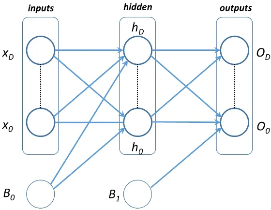
Figure 1: A Simple Feed Forward Neural Network. The nodes in the input layer is the input data, while the nodes in the hidden and output layers are perceptrons. Each

connection between nodes represents a weighted connection. ...4

Figure 2: Diagram illustrating the relationship between the input and layers. Each resulting feature map in the hidden layer uses its own convolutional filter. The filters process the input with a sliding window that sums the convolutional results across every channel at the same coordinate. ...6

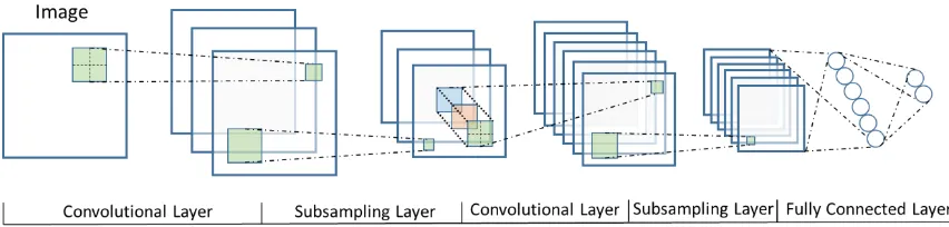
Figure 3: A visualization of the LeNet architecture. It combined convolutional, pooling, and fully connected layers to learn a model that can solve classification problems...7

Figure 4: Unrolled Recurrent Unit ...8

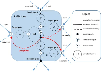
Figure 5: Long Short-term Memory Cell ...9

Figure 6: Inner Structure of a Conv-LSTM Unit ...12

Figure 7: The composite structure for unrolled LSTM unit. Blue lines represent potential conditioning ...14

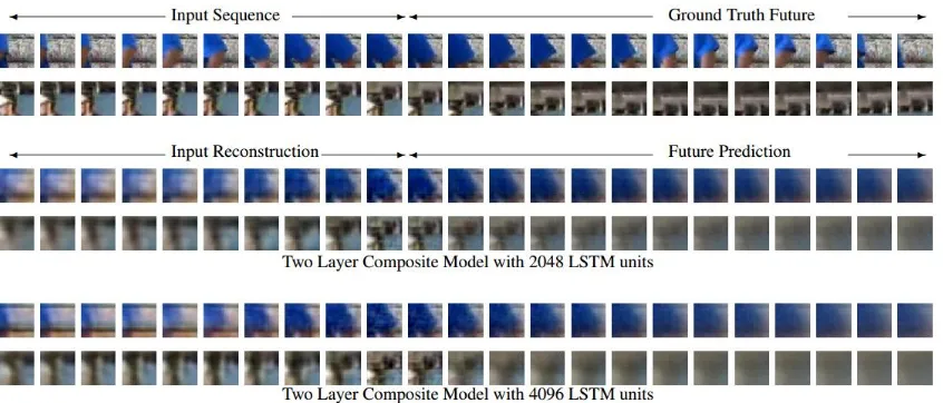
Figure 8: Reconstruction and future prediction obtained from the Composite Model on a dataset of Bouncing MNIST images [19] ...15

Figure 9: Reconstruction and future prediction obtained from the Composite Model on a dataset of natural image patches. [19] ...16

Figure 10: Two prediction examples. All of the predictions and ground truths are sampled with an interval of 3. From top to bottom: input frames; ground truth frames; prediction by the ConvLSTM forecasting network. [17]...17

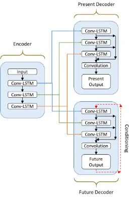
Figure 11: High-level view of the Conditioned Composite Conv-LSTM Encoder-Decoder. The right side is the encoder, while the left is the decoder. The decoder is split into a present and future decoder, where the future decoder is potentially conditioned with the output of the current time-step feeding into the input of the next. ...20

input of the next. The full composite model has a duplicate of the decoder with the target output being the input frames. ...23

Figure 13: Three samples of the first ten frames from three sequences of the Bouncing MNIST dataset ...31

Figure 14: Images from the UCSD Pedestrian dataset. The left and right columns are from the Pedestrian 1 and 2 subsets respectively...32

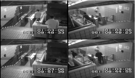
Figure 15: Images from the Subway dataset. The left and right columns are from the Exit and Entrance videos respectively. ...32

Figure 16: Images from the Avenue Dataset. ...33

Figure 17: A comparison between prototype network outputs. Each column denotes a time-step sequentially from left to right starting at T+1. Each row from top to bottom represent the input sequence, the target ground truth future sequence, the forecasting model [17], the encoder-decoder prototype, and the autoencoder prototype. ...35

Figure 18: Input reconstruction obtained from the Composite Conv-LSTM Autoencoder Model on a non-anomalous sequence from test clip 1 of the UCSD Pedestrian 1 dataset. The first row is the input ground truth video sequences, while the second is the input reconstruction. Each column denotes a time-step. Regions of interest that change through time are highlighted by a yellow bounding box. ...40

Figure 19: Future prediction obtained from the Composite Conv-LSTM Autoencoder Model on the non-anomalous sequence from test clip 1 of the UCSD Pedestrian 1 dataset used in Figure 18. The first row is the future ground truth video sequences, while the second is the output prediction. Each column denotes a time-step. Regions of interest that change through time are highlighted by a yellow bounding box. ...41

Figure 20: Input reconstruction obtained from the Composite Conv-LSTM Encoder-Decoder Model on a non-anomalous sequence from test clip 1 of the UCSD Pedestrian 1 dataset. The first row is the input ground truth video sequences, while the second is the input reconstruction. Each column denotes a time-step. Regions of interest that change through time are highlighted by a yellow bounding box. ...41

time-step. Regions of interest that change through time are highlighted by a yellow bounding box. ...42

Figure 22: Input reconstruction obtained from the Composite Conv-LSTM Encoder-Decoder Model on an anomalous sequence from test clip 1 of the UCSD Pedestrian 1 dataset. The first row is the input ground truth video sequences, while the second is the input reconstruction. Each column denotes a time-step. Regions of interest that change through time are highlighted by a yellow bounding box. ...43

Figure 23: Future prediction obtained from the Composite Conv-LSTM Encoder-Decoder Model on the anomalous sequence from test clip 1 of the UCSD Pedestrian 1 dataset used in Figure 22. The first row is the future ground truth video sequences, while the second is the output prediction. Each column denotes a time-step. Regions of interest that change through time are highlighted by a yellow bounding box. ...43

Figure 24: Input reconstruction obtained from the Composite Conv-LSTM Encoder-Decoder Model on an anomalous sequence from test clip 29 of the UCSD Pedestrian 1 dataset. The first row is the input ground truth video sequences, while the second is the input reconstruction. Each column denotes a time-step. Regions of interest that change through time are highlighted by a yellow bounding box. ...45

Figure 25: Future prediction obtained from the Composite Conv-LSTM Encoder-Decoder Model on the anomalous sequence from test clip 29 of the UCSD Pedestrian 1 dataset used in Figure 24. The first row is the future ground truth video sequences, while the second is the output prediction. Each column denotes a time-step. Regions of interest that change through time are highlighted by a yellow bounding box ...45

Figure 26: A comparison between the original and improved model’s regularity scores for testing clip 36 of the UCSD Pedestrian 1 dataset...50

Figure 27: Regularity score (Eq.7) of test clip 29 of the UCSD Pedestrian 1 dataset. Distinct local minima are represented by a blue dot, distinct local maxima are represented by a red dot, the anomalous ground truth regions are highlighted in red, and the proposed anomalous regions are highlighted in green. ...50

Figure 28: Anomaly evaluation graphs of test clips from the UCSD Pedestrian 1 dataset. Smaller areas of interest are highlighted with a yellow bounding box. ...51

Figure 29: Regularity score (Eq.7) of test clip #2 of the UCSD Pedestrian 2 dataset ...53

Figure 31: Input reconstruction obtained from the (224x224) Composite Conv-LSTM Encoder-Decoder Model on an anomalous sequence from test clip 1 of the UCSD Pedestrian 2 dataset. The first row is the input ground truth video sequences, while the second is the input reconstruction. Each column denotes a time-step. Regions of interest that change through time are highlighted by a yellow bounding box. ...55

Figure 32: Future prediction obtained from the (224x224) Composite Conv-LSTM Encoder-Decoder Model on the anomalous sequence from test clip 1 of the UCSD Pedestrian 2 dataset used in Figure 32. The first row is the future ground truth video sequences, while the second is the output prediction. Each column denotes a time-step. Regions of interest that change through time are highlighted by a yellow bounding box ...55

Figure 33: Regularity score (Eq.7) of frames 40,000–60,000 of the subway entrance. Distinct local minima are represented by a blue dot, distinct local maxima are represented by a red dot, the anomalous ground truth regions are highlighted in red, and the proposed anomalous regions are highlighted in green. ...57

Figure 34: Regularity score (Eq.7) of frames 100,000-120,000 (top) and 120,000 – 144,000 (bottom) from the Subway Entrance video. ...57

Figure 35: Input reconstruction obtained from the (224x224) Composite Conv-LSTM Encoder-Decoder Model on an anomalous sequence from the Subway Entrance video. The first row is the input ground truth video sequences, while the second is the input reconstruction. Each column denotes a time-step. ...58

Figure 36: Future prediction obtained from the (224x224) Composite Conv-LSTM Encoder-Decoder Model on the anomalous sequence from the Subway Entrance video used in Figure 35. The first row is the future ground truth video sequences, while the second is the output prediction. Each column denotes a time-step. ...58

Figure 37: Regularity score (Eq.7) of frames 37,500–52,500 of the subway exit video. ..60

Figure 38: Regularity score (Eq.7) of frames 7,500-22,500 (top) and 22,500 – 37,500 (bottom) from the Subway Entrance video. ...60

Figure 40: Future prediction obtained from the (224x224) Composite Conv-LSTM Encoder-Decoder Model on the anomalous sequence from the Subway Exit video used in Figure 39. The first row is the future ground truth video sequences, while the second is the output prediction. Each column denotes a time-step. Regions of interest that change through time are highlighted by a yellow bounding box. ...61

Figure 41: Input reconstruction obtained from the (224x224) Composite Conv-LSTM Encoder-Decoder Model on an anomalous sequence from test clip 1 of the Avenue dataset. The first row is the input ground truth video sequences, while the second is the input reconstruction. Each column denotes a time-step. ...63

Figure 42: Future prediction obtained from the (224x224) Composite Conv-LSTM Encoder-Decoder Model on the anomalous sequence from the Avenue test clip used in Figure 41. The first row is the future ground truth video sequences, while the second is the output prediction. Each column denotes a time-step...63

Figure 43: Anomaly evaluation graphs of test sequences from the Avenue dataset. ...64

List of Tables

Table 1: A comparison of Loss between the prototype networks trained on the Bouncing MNIST dataset. ...35

Table 2: Comparing reconstruction accuracy performance ...37

Table 3: Comparing reconstruction accuracy performance ...40

Table 4: Comparing anomaly detection performance of the proposed models on UCSD Pedestrian 1 dataset. There are a total of 40 anomalous events. ...47

Table 5: Average MSE per frame when evaluated on 64x64 pixel images using the specified parameters...48

Table 6: Comparing abnormal event detection performance across multiple datasets.

Ours is the Composite Conv-LSTM Encoder-Decoder (64x64) model. * Improved

Glossary

LSTM Long Short-Term Memory

Conv-LSTM Convolutional Long Short-Term Memory

FC-LSTM Fully Connected Long Short-Term Memory

CNN Convolutional Neural Network

RNN Recurrent Neural Network

MSE Mean Squared Error

FC-LSTM Fully Connected Long Short-Term Memory

ReLU Rectified Linear Unit

TP True Positive

Chapter 1

Introduction

Anomalies in videos are broadly defined as events that are unusual and signify

irregular behavior. Detecting such irregularities is important, as errors and bugs must first

be found before they can be addressed. Consequently, anomaly detection is an extensive

field that can be applied in many different areas. One such area is in computer vision

detecting irregular activities of interest in videos and can be applied to many real-world

scenarios including surveillance and security.

Meaningful events that are of interest in long video sequences, such as surveillance

footage, often have an extremely low probability of occurring. As such, manually detecting

such events, or anomalies, is a very meticulous job that often requires more manpower than

is generally available. This has prompted the need for automated detection and

segmentation of sequences of interest [1]-[15].

In contrast to the related field of action recognition where events of interest that are

clearly defined, anomalies in videos are often vaguely defined and may cover a wide range

of activities. Since it is less clear-cut, models that can be trained using little to no

supervision, including spatio-temporal features, dictionary learning and autoencoders [15]

are more applicable to the problem of evaluating anomalies. The methodologies used by

[1]-[15] were developed to detect anomalies within video sequences specifically and are

effective in doing so. A description of these methodologies and their limitations are

1.1. Thesis Contributions

This thesis aims to make two main contributions. The first is the development of a

model architecture able to encode an input video sequence, reconstruct it, and predict the

subsequent sequence. Two such networks are proposed, an encoder-decoder and an

autoencoder based model. The model utilizes Convolutional Long Short-Term Memory

(Conv-LSTM) units that allow the neural network to better learn spatio-temporal features.

Conv-LSTM units merge convolutional operations into traditional fully connected LSTM

(FC-LSTM) units, and are further discussed in Section 2.3.2. The second is the ability to

detect anomalous video segments through the model’s output using a regularity evaluation

algorithm. The regularity of a video sequence is relative to other sequences of the same

source. A preliminary investigation on the validity of the network architectures using

simplified versions are evaluated on the Bouncing MNIST dataset. The proposed networks

are then evaluated on the UCSD Pedestrian 1 dataset. The best model is improved upon

and further evaluated on the UCSD Pedestrian 2 dataset, Subway dataset, and Avenue

dataset.

1.2. Thesis Outline

This document is organized as follows: Chapter 2 discusses the prior work relative

to the thesis domain and its influence on the proposed design. Chapter 3 discusses the

proposed architectures, their various implementations, and the evaluation algorithm. The

proposed architectures include a Conv-LSTM Autoencoder and a Conv-LSTM

results on various datasets. Chapter 5 provides a conclusion summarizing the potential and

Chapter 2

Background

2.1. Feed Forward Neural Networks

The Artificial Neural Network was first proposed by Rosenblatt in 1958 [32]. Neural

networks are a biologically inspired model simulating the way a brain works. It connects

multiple “neurons,” such that each individual neuron performs simple functions that

include a nonlinearity, to model more complex tasks. A typical feed forward neural

network consists of an input layer, output layer, and one or more hidden layers (Figure 1).

The hidden and output layers are made up of perceptrons that weight their input

connections and only activate when the values used within the unit’s function exceed a

given threshold value. Every perceptron’s weights are updated through a backpropagation

algorithm that aims to minimize the error between network output and target value.

Since the network learns its own weights, it is able to determine on its own what

features are important and applicable to the task. While a strong tool, feed forward neural

networks utilizing only perceptrons are not as effective on problems that rely on spatial or

temporal information. This weakness has led to the development of Convolutional and

Recurrent Neural Networks [39].

2.2. Convolutional Neural Networks

Images and videos of similar articles are subject to inconsistency in properties that

include translation, rotation and scaling. As such, invariance to transformations is a

desirable property in any neural network dealing with vision. Invariance can generally be

introduced into models in three ways: pre-processing the data to be invariant so any

subsequent manipulation of the data will remain invariant, use regularization techniques

like tangent propagation to penalize transformed data, and building the invariance

properties into the network’s structure [21]. The Convolutional Neural Network (CNN)

initially proposed by LeCun [22], uses the third approach.

Convolutional Neural Networks (Figure 2) utilize three mechanisms: local

receptive fields, weight sharing, and subsampling. The local receptive fields are organized

into a plane called a feature map, with every field sharing the same weight. Each field

captures local patterns within an image by connecting each neuron only to small regions of

the input. This takes advantage of the fact that pixels that are close to one another are more

strongly correlated than pixels that are far apart. Since the local receptive fields share the

of the weight kernel with the sampled region of image pixel intensities. The neurons

making up a plane are known as the convolutional layer. Sliding the local receptive field

across the entire image allows features to be found regardless of position.

As the weights of a local receptive field are the same for each neuron in the

convolutional layer, it can be seen that the convolutional layer is just an image convolution

of the previous layer. The weights are therefore specified by the convolutional filter, and

are learned alongside a bias. When the input is made up of multiple channels, the neuron

becomes the summation of convolutional operations across all channels within the same

region.

Figure 2: Diagram illustrating the relationship between the input and layers. Each resulting feature map in the hidden layer uses its own convolutional filter. The filters process the input with a sliding window that sums the convolutional results across every channel at the same coordinate.

The output of the convolutional layer feeds into a sub-sampling layer that computes

a function of sub-regions of the input. The function is generally an average or maximum,

through a sample-based discretization process [20]. This helps prevent overfitting from

highly detailed representations of the topic and reduces the complexity of the problem. The

output also becomes invariant to small changes in rotation and translation [21]. Its smaller

size also decreases the complexity of the problem. This layer is generally followed by a

fully connected layer when performing classification problems. Convolutional neural

networks are not limited to two-dimensions. Networks for multi-dimensional data are

possible as long as the filter sizes are adjusted accordingly. It should be noted that a fully

connected layer can be thought of as a special case of a convolutional layer, where the filter

size is equal to the input size, and only a single convolution is performed.

Figure 3: A visualization of the LeNet architecture. It combined convolutional, pooling, and fully connected layers to learn a model that can solve classification problems.

2.3. Recurrent Neural Networks

Neural networks generally work under the assumption that the inputs are

independent from one another. This limits their effectiveness when applied to tasks that

may require the use of sequential information. A variety of Recurrent Neural Networks

(RNN) have been proposed, [21], [24], and [25], all of which create an internal network

evaluation of activation of current neurons, thereby allowing past data to influence current

outputs (Figure 4). This means that recurrent neural networks can learn temporal patterns

in data sequences. They have been applied to problems such as text generation where the

network learns to predict the next character or word based on the input text sequence [38].

Unfortunately, RNNs are limited in the range of context they retain and suffer from the

vanishing gradient problem, making it difficult to perform tasks with more than ten time

steps between the target and relevant inputs.

Figure 4: Unrolled Recurrent Unit

2.3.1 Long Short-Term Memory

The long short-term memory (LSTM) architecture seeks to overcome the

limitations of the typical RNN by adding the ability to selectively remember and forget

previous data. First proposed by [15], it has since been used in applications dealing with

sequences that require a way to discriminatively select what should be remembered. The

long short-term memory cell, as seen in Figure 5, utilizes three gates that control the

information received, retained, and output by the cell to find and exploit long-term

Figure 5: Long Short-term Memory Cell

There are three unique activation functions, the input, output, and gate activation

functions. The former two usually use a tanh activation function, while the latter, denoted

in the Figure 5 as “σ”, is always a sigmoid activation function. The gate activations are

calculated using a logistic sigmoid function of the dot product of the input and weights,

with each gate containing its own weights. The weights are shared by the unit through each

time step. The cell and hidden states are controlled by a input and output gates. The input

gate controls whether or not the input is considered, the forget gate controls whether or not

the previous cell data is considered, and the output gate controls if the current cell

information is released to the next state. The formulation of the LSTM cell can be

summarized as shown in (1) through (5). The inputs, outputs, and weights all represent a

Element-wise multiplication operations are denoted by “∘”. The input, forget, cell, output, and

hidden states for each timestep are denoted by i, f, c, o, and h, respectively, σ represents the

activation functions, and the connections between the input and each state in the LSTM

unit are denoted by a set of weights, W. The output state controls the information that is

propagated from the previous timestep, while the hidden state is the actual output of the

LSTM unit. The peephole connections allow the LSTM unit to access and propagate

information recorded from the preceding timestep. An LSTM encoder-decoder model was

used by [19] to reconstruct and predict video sequences. While It performed reasonably

well on Bouncing MNIST video sequences, it was less effective on patches of natural

images taken from the UCF-101 dataset [28]. The reconstructed images were fuzzy while

the predictions were little more than colored blobs. This is likely due to the fact that spatial

information within the data is lost while it propagates temporally though the unit. However,

[28] does use the weights from the encoder trained on the UCF-101 dataset to initialize an

LSTM classifier that performed well on in.

𝑖_𝑡 = 𝜎(𝑊_𝑥𝑖𝑥_𝑡+ 𝑊_ℎ𝑖ℎ_𝑡−1+ 𝑊_𝑐𝑖∘ 𝑐_𝑡−1+ 𝑏_𝑖) (1)

𝑓𝑡 = 𝜎(𝑊𝑥𝑓𝑥𝑡+ 𝑊ℎ𝑓ℎ𝑡−1+ 𝑊𝑐𝑓∘ 𝑐𝑡−1+ 𝑏𝑓) (2)

𝑐_𝑡 = 𝑓_𝑡∙ 𝑐_𝑡−1+ 𝑖_𝑡∘ (𝑊_𝑥𝑐𝑥_𝑡+ 𝑊_ℎ𝑐ℎ_𝑡−1+ 𝑏_𝑐) (3)

𝑜_𝑡 = 𝜎(𝑊_𝑥𝑜𝑥_𝑡+ 𝑊_ℎ𝑜ℎ_𝑡−1+ 𝑊_𝑐𝑜∙ 𝑐_𝑡−1+ 𝑏_𝑜) (4)

ℎ_𝑡 = 𝑜_𝑡∘ tanh⁡(𝑐_𝑡) (5)

2.3.2 Convolutional Long Short-term Memory

The Convolutional Long Short-term Memory architecture has been recently utilized by Shi

the usual fully connected LSTM (FC-LSTM) by using convolution for both

input-to-hidden and input-to-hidden-to-input-to-hidden connections. The formulation of the Conv-LSTM unit can be

summarized with (6) through (10). While the equations are similar in nature to (1) through

(5), the input x is fed in as images, while the set of weights for every connection is replaced

by convolutional filters. This allows the Conv-LSTM unit to keep track of less weights and

perform convolutional operations that yield better spatial feature maps. The Conv-LSTM

is more advantageous when working with images than the FC-LSTM due to its ability to

propagate spatial characteristics temporally through each Conv-LSTM state.

𝐼 = 𝜎(𝑊_𝑋𝐼∗ 𝑋_𝑡+ 𝑊_𝐻𝐼∗ 𝐻_𝑡−1+ 𝑊_𝐶𝐼∘ 𝐶_𝑡−1+ 𝑏_𝐼) (6)

𝐹_𝑡= 𝜎(𝑊_𝑋𝐹∗ 𝑋_𝑡+ 𝑊_𝐻𝐹∗ 𝐻_𝑡−1+ 𝑊_𝐶𝐹∘ 𝐶_𝑡−1+ 𝑏_𝐹) (7)

𝐶_𝑡 = 𝐹 ∙ 𝐶 + 𝑖_𝑡∘ (𝑊_𝑋𝐶∗ 𝑥_𝑡+ 𝑊_𝐻𝐶∗ ℎ_𝑡−1+ 𝑏_𝐶) (8)

𝑂𝑡 = 𝜎(𝑊𝑋𝑂∗ 𝑋𝑡+ 𝑊𝐻𝑂 ∗ 𝐻𝑡−1+ 𝑊𝐶𝑂∙ 𝐶𝑡−1+ 𝑏𝑜) (9)

𝐻𝑡= 𝑂 ∘ tanh⁡(𝐶𝑡) (10)

Convolutional and element-wise multiplication operations are denoted by “∗” and

“∘” respectively. Similar to the LSTM unit, the input, forget, cell, output, and hidden state

of each timestep are denoted by I, F, C, O, and H respectively, the activation by σ, and the

weighted connections between states by a set of weights, W. However, each state is now a

matrix representing the image, while the set of weights W is a convolutional filter. Just as

the convolutional filters of the input-to-hidden connections determine the resolution of

feature maps created from the input, the convolutional filter size of the hidden-to-hidden

connections determine the aggregate information the Conv-LSTM unit receives from the

previous time-step. The transition of states between time-steps for a Conv-LSTM unit can

capture faster motions while smaller transitional kernels capture slower motions [17]. A

visualization of the process can be seen below in Figure 6. The size of the convolutional

filters in the input-to-hidden and hidden-to-hidden connections may differ depending on

both the size and speed of the observed objects. The models used in [17] and [18] are able

to successfully reconstruct a recognizable prediction of an input video sequence from the

bouncing MNIST dataset [19]. Patraucean et al. however, does not make use of peephole

connections, showing that the effectiveness of such connections in an LSTM architecture

is debatable [18]. It should be noted that a FC-LSTM can be thought of as a special case of

a Conv-LSTM, where the filter size is equal to the input image and only a single

convolutional operation is performed, and that each Conv-LSTM unit shares the same

parameter through all time-steps.

Figure 6: Inner Structure of a Conv-LSTM Unit

The models in [17] and [18] are able to successfully reconstruct a recognizable

prediction of an input video sequence from the bouncing MNIST dataset [19]. The model

effectiveness of such connections in an LSTM architecture is still unresolved. It should be

noted that a FC-LSTM can be thought of as a special case of a Conv-LSTM, where the

filter size is equal to the input image and only a single convolutional operation is

performed.

2.4. Future Video Prediction

Long Short-Term Memory networks are capable of learning long-term

dependencies. As such, they are able to extrapolate temporally sequential data given certain

inputs. Srivastava et al. [19] takes advantage of this property to train a composite

encoder-decoder model able to reconstruct the past and predict the future video sequences. More

specifically, the encoder maps an input video representation to a fixed length

representation, while the decoder extrapolates the learned encoding into the past and future

video sequences. When using only a normal encoder-decoder model, the target values of

the model determine what the model can be used for. When the target output is of the input,

the model is able to create a reconstruction of the input video sequence. When the target

output is of subsequent frames, however, the model learns to predict the subsequent video

sequence.

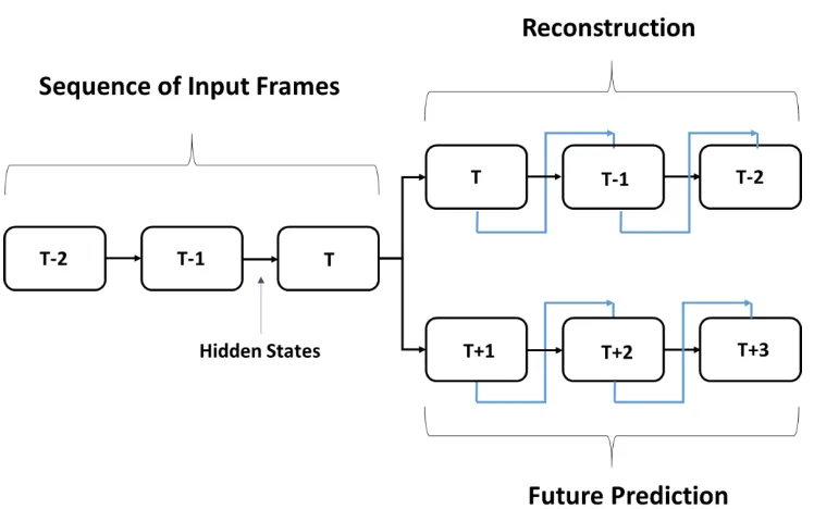
The model is further improved by combining both the reconstruction and prediction

models into a composite model, using both the current and future video sequences as target

outputs and potentially conditioning each step with the output of the previous

time-step (Figure 7). Reconstruction models have the tendency to learn trivial representations

the most recent frames, as they are generally the most immediately relevant, i.e, {vt-1, . . .

,vt-k} are more important than v0 when predicting vt While this is effective for specific

predictions, the loss of information from older time-steps will lead to less accurate

predictions for more general video sequences during testing. The reconstruction of both the

past and future video sequences forces the learned encoding to contain more meaningful

data, thus improving the overall performance of the system.

Figure 7: The composite structure for unrolled LSTM unit. Blue lines represent potential conditioning

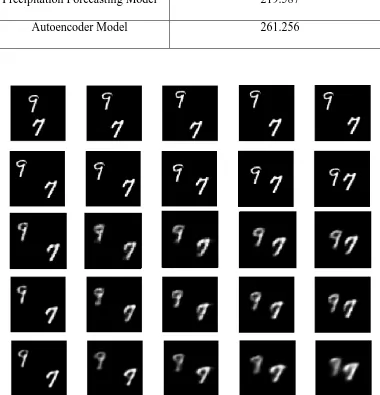
Srivastava et al. evaluates his proposed model on the Bouncing MNIST dataset,

comprised of 64x64 grayscale images (Figure 8), and a set of 32x32 natural image patches

(Figure 9) from the UCF-101 dataset [28]. It is able to successfully reconstruct and predict

a sequence of images accurately on the Bouncing MNIST images, with the best

reconstruction nor the prediction maintaining spatial resolution. The input reconstruction

does show a blurred approximation of both structure and motion though time, but the future

prediction loses cohesion in both by the fourth time-step. While the reconstructions get

sharper when more LSTM units are added to each layer, the predictions remain the same,

showing the model’s inability to extrapolate the future from the encoding. The results by

Srivastava et al. show that while the model is effective on simple synthetic images, it is

unable to learn and temporally propagate spatial features on more complex images,

regardless of size.

Figure 9: Reconstruction and future prediction obtained from the Composite Model on a dataset of natural image patches. [19]

Shi et al. propose the use of Convolutional LSTMs with the encoder-decoder

structure for future video prediction that is able to better retain spatio-temporal information.

Its decoder is unique in that it performs a 1x1 convolutional operation across the output of

each layer to obtain an output, as opposed to looking solely at the last layer. The proposed

architecture was shown to outperform the LSTM models used by [19] when predicting

future video sequences for a synthetic Bouncing MNIST Dataset. It was also successfully

applied to a precipitation forecasting problem that used satellite imagery of clouds to

predict weather patterns (Fig. 10), showing its applicability in predicting non-synthetic

Figure 10: Two prediction examples. All of the predictions and ground truths are sampled with an interval of 3. From top to bottom: input frames; ground truth frames; prediction by the ConvLSTM forecasting network. [17]

2.5. Anomaly Detection in Videos

When labels are provided as a ground truth for anomalous actions, anomaly

detection is a problem that can be evaluated by building predictive models and considering

a binary classification problem. However, such labels are often uncommon, or unwieldy,

and the data available for training a model are limited to containing little to no anomalous

events. The available training data often result in the formulation of semi-supervised

models that can be adapted to operate in an unsupervised mode by using a sample of the

unlabeled data set as training data. Scoring techniques can be used to evaluate the output

of the models on testing data and used to label the data using domain-specific thresholds

[16].

Such techniques have been used to great effect in [5], [19], [1], [18], and [4], where

models are trained with little to no supervision and used to classify anomalous sequences

in a given video. Handcrafted features comprised of a mixture of dynamic textures and

spatial anomaly maps are used by Cong et al. in [5] to learn the “normalcy” of a video

in [19] by creating a probability distribution of low-level observations. Given a new

observation, it can calculate the likelihood of occurrence to determine whether or not it is

anomalous. The issue with hand-crafted features is that they may be too specialized, which

makes them unable to adapt to or learn unexpected events effectively. Neural networks

deal with this issue by allowing the network to learn what features are important. Zhao et

al. utilizes an unsupervised dynamic sparse coding algorithm in [1] to train dictionaries

with which anomalies are detected through the reconstruction error. Lu et al. improves

upon this in [18] by introducing an approach that directly learns sparse combinations

instead of a dictionary, thereby significantly speeding up testing. While sparse coding has

been shown to be effective, dictionaries may still contain unused or noisy elements within

the dictionary, reducing their effectiveness. Hasan et al. employs a convolutional neural

network in [4] to learn the temporal regularity of given video sequences. A regularity score

is computed from the reconstruction error and used to detect anomalous segments. While

effective, convolutional neural networks were not developed with temporal features in

Chapter 3

Anomaly Detection through Future Prediction

This chapter describes the approach used to perform anomaly detection through

future prediction using convolutional long short-term memory units. The proposed

approach is inspired by the idea that an encoder-decoder model will be able to learn and

reconstruct “regular” video sequences from the training data. This will force anomalous

data to be more difficult to reconstruct with each subsequent time-step due to error

propagation. The design of the proposed architectures used to predict future video

sequences are discussed in Section 3.1, and the evaluation algorithms used to identify

anomalous video segments is discussed in Section 3.2.

3.1. Proposed Architectures

Convolutional LSTM (Conv-LSTM) units have recently been proposed and used

by [17] and [18] (Section 2.3.2). It takes advantage of the spatial information retained by

training convolutional weights to better propagate spatial features temporally in the LSTM.

These units have been utilized to create two distinct network architectures, a Composite

Conv-LSTM Encoder Decoder, described in Section 3.1.1, and a Composite Conv-LSTM

Autoencoder, described in Section 3.1.2. The results can be found in Section 4.

3.1.1 Proposed Composite Convolutional LSTM Encoder-Decoder

The architecture is inspired by the models discussed in Section 2.4. The network

by Shi et al. utilizes only a future encoding-decoder model to predict future video

sequences, while the model by Srivastava et al. utilizes a composite conditioned structure,

but is comprised of FC-LSTM units. The proposed architecture utilizes multiple stacked

parts, the encoder, and the decoder. A high level view of the proposed model using three

Conv-LSTM layers can be seen in Figure 11.

Figure 11: High-level view of the Conditioned Composite Conv-LSTM Encoder-Decoder. The right side is the encoder, while the left is the decoder. The decoder is split into a present and future decoder, where the future decoder is potentially conditioned with the output of the current time-step feeding into the input of the next.

3.1.1.1

Encoder

The encoder accepts a sequence of reshaped frames in chronological order as input.

non-overlapping patches, the model will lose detail but learn more significant data. Each

Conv-LSTM layer is made up of multiple Conv-Conv-LSTM units that span across the specified

number of time-steps. The outputs of the last time-step of each Conv-LSTM layer are used

as the encoding. Unlike traditional convolutional neural networks [10], the proposed model

does not utilize max-pooling layers. It instead feeds the output of each Conv-LSTM layer

directly into the next one, allowing each subsequent layer to accrue temporal changes and

focus on different features.

3.1.1.2

Decoder

The decoder is split into two parts, the past, and the future. The past decoder

reconstructs the input video segment, while the future decoder creates a prediction of what

the future video segment will be. The first time-step of both portions of the decoder are

initialized with the same encoding provided by the corresponding layers of the encoder.

The past decoder does not use anything as input to the first layer, and the output is

determined solely from the information extracted from its initialization. The outputs of

each layer are concatenated together and summed through a 1x1 convolutional filter to

obtain the reconstruction of the input. This final step essentially forces each layer to

represent the same set of input patches at different temporal features. The first layer is the

most static and will focus on still objects while the last layer will focus on larger

movements. We consider two options for the future decoder, one in which it is not

conditioned, and one in which it is. An unconditioned decoder has the same architecture as

the past decoder. A conditioned decoder uses the summed output of each time-step as the

input to the first layer of the subsequent time-step, thus “conditioning” it to the previous

As stated in [19], only the future decoder is conditioned, because the past only has

one possible outcome, while the future may vary. Conditioning potentially limits the

variation by providing more information from the previous time-step. The proposed

architecture uses a composite conditioned structure comprised of Conv-LSTM units. By

combining the approaches taken by Shi et al. and Srivastava et al., a better prediction can

be obtained for more accurate reconstruction errors. This potentially allows the model to

better learn a video’s normality, thus making anomalous video segments containing

sequences that are hard to reconstruct more likely to stand out.

3.1.2 Proposed Conv-LSTM Autoencoder

This architecture is inspired by the convolutional autoencoder network used by

Hasan et al, and is adapted for future prediction by the inclusion of an additional encoder.

The proposed architecture utilizes multiple stacked Conv-LSTM layers in conjunction with

max-pooling layers in an end-to-end trainable model. The design utilizes a two-step

encoder-decoder format, where the decoder is structured as an autoencoder (Fig. 12). The

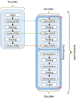
Figure 12: High-level view of the Conditioned Conv-LSTM Autoencoder. The right side is the encoder, while the left is the decoder. The decoder uses an autoencoder format and is conditioned with the output of the current time-step feeding into the input of the next. The full composite model has a duplicate of the decoder with the target output being the input frames.

3.1.2.1

Encoder

A sequence of frames is used as input to the first Conv-LSTM layer. It is then

immediately followed by a max-pooling layer. The max-pooling layer helps consolidate

the activation of neurons representing the features while increasing spatial invariance and

reducing dimensionality. The output is then fed back into any additional Conv-LSTM

layers, with the process repeating. This allows the features within large images to found

Conv-LSTM layer is an encoding and used to initialize the corresponding Conv-Conv-LSTM layers of

the decoder.

3.1.2.2

Decoder

The decoder employs an autoencoder structure, with its own encoder and decoder.

The encoder portion utilizes the same structure as the first encoder, but initializes its

Conv-LSTM layers with the encoding of the corresponding layer from the encoder. This encoder

is responsible for transforming the initialization into a traditional convolutional

autoencoder encoding at each time-step. The new encoding at each time-step is decoded

through deconvolution followed by unpooling layers to restore the image to its former size.

The deconvolution weights are tied to the input-to-cell convolutional weights from the

respective Conv-LSTM layer. Two decoders are also employed, one for the past input

video sequence, and one for the future prediction. As with the Encoder Decoder model, we

consider both an unconditional and a conditional structure for the future decoder. The

conditioned decoder accepts the output of the last layer in the previous time-step as the

input to the first layer of the current time-step.

It should be noted that this architecture does not utilize tied weights between the

encoding and decoding portions of the autoencoder. This is due to the fact that the input of

the encoder portion is not the same as the output of the decoder, as the architecture

extrapolates the future.

3.1.3 Parameters of Note

The proposed architecture has many more parameters than a convolutional or

size of each connection in a Conv-LSTM unit, the number of Conv-LSTM units in a layer,

the number of layers, the input and target segment lengths, and the patch size by which a

frame is reshaped.

The number of Conv-LSTM layers is important in that it determines the number of

chances temporal information have to be transmitted in a model. For instance, the third

time-step in the first layer could only receive information from the input and the previous

two time-steps. The same time-step at the third layer would receive the same, but the input

of each step from the second layer may receive information from the previous

time-steps of that layer. At the same time, only so many layers can be added before the data

propagated through time becomes redundant. The input-to-hidden filters serve a similar

purpose to the convolutional filters in traditional convolutional neural networks. As

discussed in Section 2.3.2 however, the filter size of hidden-to-hidden connections is

responsible for both controlling the propagation of information between states and

capturing motion between frames. It is therefore important to examine the speed of objects

in the target domain when selecting this parameter.

The input and target lengths determine the amount of information to be encoded

and extrapolated, respectively. The longer the input length is, the more information it will

have to learn, i.e. what data is meaningful and should be propagated into the encoding. At

the same time, this comes at the cost of additional parameters that increase the memory

and computational cost. Conversely, a longer output requires more information to be

extrapolated from a single encoding. The patch size determines the complexity of the

model.A large patch size will result in more detailed feature maps. However, not all

down into smaller motions that can be modeled together. A larger patch size is therefore

more likely to produce more noise and contain non-essential information.

It is also important to select a proper non-linearity function to prevent the issue of

vanishing gradients, a suitable loss function to calculate the deviation between the target

and model outputs, and an appropriate update function to learn weights efficiently.

3.2. Evaluation Algorithm

A trained model can be used to obtain a reconstruction of the input video sequence and

prediction of its subsequent frames. This reconstruction can be visualized for a qualitative

inspection by the user, or quantified for use in evaluation algorithms. In a qualitative

inspection of the reconstruction and predictions, anomalous events will be more likely to

stand out, as the trained model does not have the necessary information to properly

reconstruct or predict it. For a quantitative assessment, the reconstruction and prediction

errors will be recorded and used in an evaluation algorithm. The reconstruction error, e, is

obtained by taking the total Mean Squared Error (MSE) as defined in Eq. (11), where 𝜃̂ is

the pixel value of the model’s output, 𝜃 is the target value, n is the number of pixels per

frame, and p is the number of frames.

⁡⁡⁡⁡⁡⁡⁡⁡⁡⁡⁡⁡⁡⁡⁡⁡⁡⁡⁡⁡⁡⁡⁡⁡⁡⁡⁡⁡⁡⁡⁡⁡⁡⁡⁡⁡⁡⁡⁡⁡⁡⁡⁡⁡⁡⁡⁡⁡𝑒 = ⁡ ∑ ∑(𝜃̂_𝑘𝑖− 𝜃_𝑘𝑖)2

𝑝

𝑖=1 𝑛

𝑘=1

⁡⁡⁡⁡⁡⁡⁡⁡⁡⁡⁡⁡⁡⁡⁡⁡⁡⁡⁡⁡⁡⁡⁡⁡⁡⁡⁡⁡⁡⁡⁡⁡⁡⁡⁡⁡⁡⁡(11)

The quantitative evaluation algorithm used in this thesis is based on the one used

by [19]. A regularity score is computed from the error values. The regularity score

reconstructions from the same video, as different videos may have different notions of

abnormality. The regularity 𝑔(𝑥) of a sequence can be computed as follows:

⁡⁡⁡⁡⁡⁡⁡⁡⁡⁡⁡⁡⁡⁡⁡⁡⁡⁡⁡⁡⁡⁡⁡⁡⁡⁡⁡⁡⁡⁡⁡⁡⁡⁡⁡⁡⁡⁡⁡⁡⁡⁡⁡𝑔(𝑥) = 1 −

𝑒(𝑥) − min

𝑥 ⁡𝑒(𝑥)

max

𝑥 ⁡𝑒(𝑥)

⁡⁡⁡⁡⁡⁡⁡⁡⁡⁡⁡⁡⁡⁡⁡⁡⁡⁡⁡⁡⁡⁡⁡⁡⁡⁡⁡⁡⁡⁡⁡(12)

where x is the output reconstruction sequence and 𝑒(𝑥) is the reconstruction error of that

sequence. Video sequences containing normal events will have a high regularity score since

it is similar to the data used to train the model, while sequences containing abnormal events

will have a low regularity score. Abnormal events will cause the prediction reconstructions

to diverge further from the target output, as the model will not contain information to

support it. Distinct local minima or scores below a certain threshold from a time series of

regularity scores can therefore be used to determine the location of abnormal video

sequences.

This thesis improves upon the methodology by Hasan et al. by using Conv-LSTMs

to learn better spatio-temporal features and making use of both distinct local minima and

maxima within the evaluation algorithm to determine anomalous regions more accurately.

The distinct points are found with a filter using the Persistence 1D algorithm [30]. The

algorithm finds such points by finding local minima and maxima after smoothing the

function using a biharmonic reconstruction. Distinct local minima represent video

sequences that are highly likely to contain anomalies. Regions of anomalous video

segments are proposed based on the minima found. Points that are within a certain

threshold can be considered to be part of the same anomalous sequence. Distinct local

maxima potentially represent regular video sequences that take place immediately before

limiting the length of the proposed anomalous segment. More specifically, the new

proposed region border is midway between the maxima and minima. This constraint is

precluded when the distinct maxima is between two distinct minima that are considered to

be of the same anomalous sequence. The proposed anomalous regions are recorded for

every video evaluated and compared to the ground truth. Anomalies are considered

detected if a certain percentage of the proposed detection is overlapped by the ground truth

anomaly. Multiple detections of the same anomaly are considered a single true positive

detection.

3.2.1 Parameters of Note

The evaluation algorithm has several tunable parameters. The length of the

proposed anomalous segment directly impacts how likely it is for it to overlap the ground

truth anomalous segment. A large area may include the actual anomaly, but contain large

sequences of data that are normal. Conversely, it is more likely for a small area to include

only the anomalous region, but is less likely to do so and may not encompass the entire

thing. The overlap percentage is responsible for determining if the proposed anomalies are

actually anomalies. A low percentage means that it would be correct even if only a tiny

portion of the proposal is correct, while a high percentage would require very high

precision for it to match the ground truth. The distance by which two distinct minima would

be considered of the same anomaly ties into this by affecting the area of the anomalous

segment, as it merges the proposed segments based on both minima.

anomalous video segment, while each distinct maximum helps constrain the regions for

more accuracy. It should be noted that the evaluation algorithm is more likely to be accurate

in longer video clips. Shorter videos are more likely to have anomalies near the beginning

of end of the video, thus reducing the amount of information provided and making it harder

Chapter 4

Experimental Results

4.1. Experimental Setup

The proposed system is designed, coded, and trained using Lasagne. Lasagne is a

lightweight library used to build and train neural networks in Theano. Its supports many

different neural network implementations including, but not limited to, dense networks,

Convolutional Neural Networks, and recurrent networks. It is also highly modular with

every part able to be used independently of Lasagne, transparent with its source code easily

understandable and available in Python, and easily modified. The last part is especially

important, as the source code for the Conv-LSTM unit used in [6] was not yet available

when work for this thesis was started. Caffe was considered but not chosen. While it is

easy to implement existing networks in Caffe, it is much more difficult to modify the source

code. Classes in Lasagne were modified to allow for a Conditioned Encoder-Decoder

implementation of a Conv-LSTM network.

MATLAB was chosen as the tool used to evaluate the model outputs and detect

anomalies. It is a powerful tool that allows for a quick visualization of both the regularity

scores and reconstructions. A prototype of each proposed network was first tested and

evaluated to ensure that the code written was working as intended. The proposed networks

were then evaluated to determine the most effective one. The best model was then trained

and evaluated over multiple datasets. The outputs were analyzed qualitatively through a

visualization of the past reconstruction and future prediction, and quantitatively by

comparing the average loss and detection rates. Matlab was used to visualize the

4.1.1 Dataset Selection

The datasets used in the experiments are the Bouncing MNIST dataset [19], UCSD

Pedestrian Datasets [8], Avenue Dataset [14], and Subway Datasets [3]. The results used

for comparison were obtained from [15] and [9].

The Bouncing MNIST dataset is a synthetic dataset comprised of 10,000 video

sequences, with each sequence depicting two MNIST [21] figures moving around in a

64x64 pixel area, and 20 frames long (Figure 13). It is used by [17] and [19] to show that

their models are able to predict and reconstruct future video sequences.

Figure 13: Three samples of the first ten frames from three sequences of the Bouncing MNIST dataset

The UCSD Pedestrian dataset is comprised of two subsets, Pedestrian 1 and

Pedestrian 2, that each depict the activities of a different pedestrian walkway and are further

split into training and testing data. The training data contains only the “regular” activity of

pedestrians, while the test data contains “anomalous” events including but not limited to

people skateboarding, cycling, and driving small vehicles (Figure 14).

The Subway dataset is split into two subsets, Enter and Exit (Figure 15). The first

subset depicts people entering a subway station, while the second shows them leaving.

Figure 14: Images from the UCSD Pedestrian dataset. The left and right columns are from the Pedestrian 1 and 2 subsets respectively.

The Avenue dataset captures activity on a CUHK campus avenue (Figure 16). The

images are in RGB and contain images of activity that are generally larger than those found

in the UCSD and Subway datasets. Like the other two, it also contains both a training and

testing dataset.

Figure 16: Images from the Avenue Dataset.

The Bouncing MNIST dataset is only evaluated on the baseline Future Conv-LSTM

Encoder Decoder model seen in Section 2.4. As it was also used by [17] and [19] in their

experiments, the preliminary results obtained from it are used as a benchmark to ensure

that the base code is working correctly. While useful as an initial validation for the base

network code, it is unable to show whether or not the model is applicable to the problem

explored in this thesis. The Bouncing MNIST dataset is synthetic and simplistic, while the

videos relevant to the problem domain are all natural footage.

The UCSD Pedestrian 1 dataset was chosen as the benchmark dataset for all

experiments done in this thesis. It is used to find the most effective model by tuning the

parameters discussed in Section 4.3.1. Once the optimal model was found, it was then

4.2. Preliminary Code Validation

Prototypes of the encoder-decoder and autoencoder networks that are only able to

perform future prediction are evaluated on Bouncing MNIST data. The initial parameters

selected for the preliminary future Conv-LSTM encoder-decoder used to evaluate the

Bouncing MNIST (BMNIST) dataset are based on the parameters used in [17]. The

convolutional filter size used for both the input-to-hidden and hidden-to-hidden

connections was 5x5. Since the target pixels are either black or white, a sigmoid

nonlinearity was applied to the output of the convolutional layer, and a binary cross entropy

was used as the loss function. Three Conv-LSTM layers were used, with 256, 128, and 128

filters respectively. As in [6], RMSProp [31] with a learning rate of 10−4 and decay rate of

0.9 is used. An input and output length of five frames each was selected, as the accuracy

of the reconstructions is prioritized over an abstraction of predicted motion. As the

parameters for the Conv-LSTM Autoencoder model are similar, the same parameters are

chosen for use when applicable.

The models are compared with an implementation of the precipitation forecasting

model used by Shi et al. While it is not stated in [17], the released code by Shi et al. also

reconstructs the output of the last time-step of the input. A comparison of the average

binary cross entropy per frame between the model output and ground truth, as seen in Table

1, would show that the forecasting model performed the best while the autoencoder model

performed the worst. This is misleading because it averages in the input reconstruction

output of the encoder. A visualization of the outputs in Figure 17 shows that output of the

encoder-decoder model has a much higher resolution than the autoencoder model, whose

were evaluated to make sure the code was written correctly, they were only trained using

a mini-batch for 20,000 iterations, and the parameters were not optimized.

Table 1: A comparison of Loss between the prototype networks trained on the Bouncing MNIST dataset

Average Binary Cross Entropy Per Frame

Encoder-Decoder Model 238.406

Precipitation Forecasting Model 219.587

Autoencoder Model 261.256

4.3. Parameter Selection

4.3.1 Model Parameters

The input images are resized to 224x224 pixels and converted to grayscale. A

preliminary Conv-LSTM Encoder-Decoder baseline model was evaluated for use as

reference in parameter selection. The baseline model utilizes parameters similar to the

prototypes tested in Section 4.2, with an input length of five, output length of five, a filter

size of 5x5, three Conv-LSTM layers, and a total of 512 Conv-LSTM filters. A sigmoid

non-linearity is also applied to the final convolutional layer.

The parameters tested in variations of the baseline model include the length of both

the input and output, the filter size, and the non-linearity function (Table 2). The model

with an input length of ten outputs a slightly lower MSE per frame, but takes 1.5 times the

amount of time to train, making it largely inefficient. Furthermore, the more time-steps into

the future the model predicts, the worse each prediction becomes (Table 1). A filter size of

3x3 was considered as the objects in the datasets utilized move more slowly than the one

used by [17]. As most convolutional neural networks use a rectified linear unit (ReLU)

nonlinearity function, that is tested as well. Ultimately, the parameters used by the baseline

model are shown to be the most effective. As the parameters for the Conv-LSTM

Autoencoder model are similar, the same parameters are chosen for use when applicable.

The binary cross entropy loss function is not suitable for natural images like those

seen in the UCSD Pedestrian dataset. The loss function for the baseline model is therefore

changed to Mean Square Error. All other parameters remain the same. Evaluations using

The parameters changed include the number of layers, and the number of

Conv-LSTM units per layer. While traditional convolutional layers apply a rectified linear unit

(ReLU) nonlinearity to the output, a sigmoid nonlinearity is also considered. The total

number of units remain the same though, (i.e., one layer has 512 units, while two layers

may have 256 units in each). The input and output length are set at ten for two different

experiments. The best model parameters are then used to evaluate a composite and

conditioned composite model.

Table 2: Comparing reconstruction accuracy performance

Parameters Modified

(Input Length, Output Length, Filter Size, Output Nonlinearity)

Average MSE Per Frame

(5, 5, 5x5, Sigmoid) 20.5076

(10, 5, 5x5, Sigmoid) 17.46702

(5, 10, 5x5, Sigmoid) 23.0266

(10, 10, 5x5, Sigmoid) 24.8644

(5, 5, 3x3, Sigmoid) 30.183

(5, 5, 5x5, ReLU) 24.8302

For the UCSD Pedestrian 1 and 2 datasets, the last training video sample was held

out for validation. For the Subway and Avenue datasets that have only one video for

training, the last twentieth of the video was held out for use as validation. Early stopping

4.3.1.1

Optimization and Initialization

The cost function of eq. (11) was optimized with RMSProp [31]. It uses a running

average over the root mean squared of recent gradients to normalize the gradients and

divide the learning rate. A learning rate of 10−3 and decay rate of 0.9 are used. Adagrad

[33] and Adam [34] were both considered and tested as well, but RMSProp was empirically

chosen for its smaller resulting loss values. The learning rate is set to .0001. We use a

mini-batch of five video sequences and train the models for up to 25,000 iterations. Early

stopping is performed based on the validation loss if necessary. The weights are initialized

using the Xavier algorithm [35]. The algorithm automatically scales the initialization based

on the number of input and output neurons to prevent the weights from starting out too

small or large. This is significant, as weights that start too small cause a reduction of

variance in the output that propagate a decrease in both the weights and values until they

become too small to matter. Similarly, too large of a starting weight will cause the learned

weights and outputs to explode in magnitude [31]. It is also an important factor in speeding

up and ensuring the convergence of the network. The convolutional filters within the

input-to-hidden and hidden-input-to-hidden states in the Conv-LSTM units all use the same filter size

in this thesis. It should be noted that while units share the same parameters at each timestep,

the filter sizes of different states within the unit may differ in size if necessary.

4.3.2 Evaluation Parameters

A temporal window of fifty frames before and after distinct local minima is used

to propose anomalous regions, as most anomalous activities are approximately one hundred

be a part of same abnormal event. We consider a detected abnormal region as a correct

detection if it has at least fifty percent overlap with the ground truth. A parameter-sweep

at intervals of 0.05 is performed to determine the threshold parameter for the Persistence1D

algorithm [30]. Since abnormal events are unique to each target video domain, a different

threshold is selected for each dataset.

To make the results easier to visualize, the regularity score and its evaluation are

graphed. Distinct local minima are represented by a blue dot, distinct local maxima are

represented by a red dot, the anomalous ground truth regions are highlighted in red, and

the proposed anomalous regions are highlighted in green. It should be noted that the last

nine frames are not evaluated since the model requires a minimum of ten frames, five as

the input and five as the target, to return a reconstruction score.

4.4. Results

4.4.1 Predicting Past and Future Video Sequences

The learned models are able to successfully reconstruct the past and predict the

future. The encoder-decoder based model performs significantly better than the

autoencoder based models (Table 3), with the former an average MSE per frame of less

than a tenth of the latter. Contrary to our expectations, the unconditioned model performed

slightly better that the conditioned version. We were not able to test the conditio