Variational Models and Algorithms for Blind Image
Deconvolution with Applications
by
Bryan M. Williams
under the supervision of
Professor Ke Chen
Thesis submitted in accordance with the requirements of the University of Liverpool for the
degree of Doctor in Philosophy.
Contents
Acknowledgement . . . vi
Abstract . . . vii
List of Figures . . . ix
List of Tables . . . xix
List of Algorithms . . . xxii
Publications . . . xxiii
1 Introduction 1 1.1 Introduction to Image Deblurring . . . 1
1.1.1 The Problem of Blur Degradation of Images . . . 1
1.1.2 Modelling the Blurring Process . . . 2
1.1.3 Restoring Images from Blur Degradation . . . 3
1.2 Thesis Outline . . . 4
2 Mathematical Preliminaries 7 2.1 Normed Linear Spaces . . . 7
2.1.1 Convex Functions . . . 9
2.1.2 Differentiable Functions . . . 10
2.2 Calculus of Variations . . . 11
2.2.1 Variation of a Functional . . . 11
2.2.2 The Divergence Theorem and Integration by Parts . . . 12
2.3 Functions of Bounded Variation . . . 13
2.4 The Coarea Formula . . . 15
2.5 Inverse Problems and Regularisation . . . 16
2.5.1 Well and Ill-Posed Problems . . . 16
2.5.2 Inverse Problems . . . 16
2.5.3 Regularisation . . . 17
2.5.4 Regularisation Parameter Selection . . . 18
2.6 Image Representation . . . 18
2.6.1 Computational Representation . . . 18
2.6.2 Mathematical Representation . . . 19
2.7 Discretisation of Partial Differential Equations . . . 19
2.8.1 Convolution Theorem . . . 23
2.9 Iterative Methods for Solving Linear Systems of Equations . . . 24
2.9.1 The Jacobi Method (JAC) . . . 25
2.9.2 The Gauss-Seidel Method (GS) . . . 26
2.9.3 Lexicographic Ordering . . . 27
2.9.4 Convergence . . . 28
2.10 Iterative Solutions of Nonlinear Equations . . . 32
2.10.1 Newton’s Method . . . 33
2.10.2 Steepest Descent Method . . . 34
2.10.3 Conjugate Gradient Method . . . 34
2.10.4 Additive Operator Splitting (AOS) . . . 39
3 Review of Variational Models for Image Reconstruction 44 3.1 Introduction . . . 44
3.2 Image Denoising . . . 45
3.2.1 Gaussian Noise . . . 46
3.2.2 Other Noise Types . . . 46
3.2.3 Total Variation Denoising . . . 47
3.2.4 Alternative Regularisation . . . 48
3.3 Image Deblurring . . . 49
3.3.1 Filtering Model . . . 50
3.3.2 Variational Approach . . . 53
3.3.3 Tikhonov Regularised Deblurring . . . 54
3.3.4 L2 Regularised Deblurring . . . 55
3.3.5 Total Variation Deblurring . . . 57
3.3.6 Alternative Regularisation Models . . . 57
3.3.7 Deblurring in the Presence of Poisson Noise . . . 58
3.3.8 Semi-Blind Models . . . 61
3.4 Blind Image Deblurring (BID) . . . 64
3.4.1 You and Kaveh (1996) . . . 64
3.4.2 Chan and Wong (1998) . . . 66
3.4.3 Perrone and Favaro (2014) . . . 69
3.4.4 Matlab Deblurring . . . 70
3.4.5 Deblurring of Multi-Channel Images . . . 71
3.5 Image Segmentation . . . 74
3.5.1 Mumford-Shah Segmentation Model . . . 74
3.5.2 Chan-Vese Segmentation Model . . . 75
4 Application to Blurred Images and some Refinements 76 4.1 Initial Applications . . . 76
4.1.2 Image Deblurring given the Blur Function . . . 77
4.1.3 Solving the System and Results . . . 79
4.1.4 Alternative Boundary Conditions . . . 80
4.1.5 Image Deblurring without Knowledge of the Blur Function . . . 83
4.1.6 Conclusion . . . 88
4.2 An Accelerated Deblurring Model by Variable Splitting . . . 88
4.2.1 Dense and Non-Linear System . . . 89
4.2.2 Separating Deblurring and Denoising . . . 89
4.2.3 Experimental Results . . . 92
4.2.4 Blind Deblurring . . . 93
4.2.5 Solution Algorithm . . . 95
4.2.6 Experimental Results . . . 95
4.2.7 Conclusion . . . 97
4.3 A Constrained Kernel Filtering Model for Blind Deconvolution . . . 98
4.3.1 Simultaneous Blind Image Deblurring . . . 98
4.3.2 Optimisation Constraints for Blind Deblurring . . . 99
4.3.3 Alternative Optimisation Constraints . . . 100
4.3.4 Intensity Based Constraints for Local Support Kernels . . . 100
4.3.5 Solution Algorithm . . . 101
4.3.6 Experimental Results . . . 103
4.3.7 A Blind Deblurring Model for Gaussian Blur . . . 103
4.3.8 Location Based Constraints for Global Support Kernels . . . 104
4.3.9 Solution Algorithm . . . 106
4.3.10 Experimental Results . . . 106
4.3.11 Conclusion . . . 106
5 A New Constrained Deblurring Model 109 5.1 Introduction . . . 109
5.2 The Total Variation based Deblurring Models . . . 110
5.3 A Transform Based Method for Implicitly Constrained Reconstruction . 111 5.4 Refinements and other Solution Strategies . . . 115
5.4.1 Alternative Linearisation . . . 115
5.4.2 Alternative Regularisation . . . 115
5.4.3 Initialisation of u and k . . . 116
5.4.4 An Acceleration Algorithm for the Model . . . 116
5.4.5 A Convex Accelerated Model . . . 118
5.5 Experimental Results . . . 123
5.5.1 Methods and Test Images . . . 123
5.5.2 Error Measures . . . 124
5.5.3 Result Sets . . . 125
5.A Selection of Parameters in T(ψ) . . . 127
5.B Derivation of Total Variation Regularisation of a Transformed Function 137 6 A Robust Model for Constrained Blind Image Deblurring 139 6.1 Introduction . . . 139
6.2 The Inverse Problem and Current Models . . . 140
6.3 A Refined Blind Model . . . 144
6.3.1 Choice of Positivity Transforms . . . 144
6.3.2 Reformulation of the Blind Deblurring Model . . . 145
6.4 Solution of Non-Linear Deconvolution Equations for Model (6.7) . . . . 145
6.4.1 A Fixed Point Method . . . 146
6.4.2 Boundary conditions . . . 147
6.4.3 Kernel Constraints . . . 147
6.4.4 Numerical Implementation . . . 149
6.4.5 A Fast Splitting Method . . . 155
6.4.6 A Mixed Model Suitable for Smooth Blur Kernels . . . 156
6.5 Experimental Results . . . 159
6.6 Conclusion . . . 168
6.A Derivation of Euler Lagrange Equations for the Blind Model (6.8) . . . . 168
6.B Derivation of L2 Regularisation Term for the Mixed Model . . . 169
7 Semi-Blind Deblurring with Parametric Kernel Identification 171 7.1 Introduction . . . 171
7.2 Existing Models . . . 172
7.3 A New Model for Implicitly Constrained Semi-Blind Deconvolution . . . 173
7.3.1 Enhancement 1: Incorporating Implicit Constraints . . . 174
7.3.2 Enhancement 2: Regularisation of the Blur Function . . . 176
7.3.3 Enhancement 3: Smoothing Noise . . . 176
7.4 Constructing Alternative Blur Functions . . . 177
7.4.1 Out of Focus Blur . . . 178
7.4.2 Box Blur . . . 180
7.4.3 Linear Motion Blur . . . 184
7.4.4 Combined Equation . . . 186
7.5 Experimental Results . . . 188
7.5.1 Images . . . 188
7.5.2 Blur functions . . . 188
7.5.3 Models . . . 188
7.5.4 Measuring Error . . . 190
7.5.5 Result Sets . . . 190
8 Simultaneous Reconstruction and Segmentation of Blurred Images 202
8.1 Introduction . . . 202
8.2 Existing Methods . . . 203
8.2.1 Constrained Image Reconstruction . . . 205
8.3 Two-Stage Models for Restoring and Segmenting Blurred Images . . . . 206
8.4 A New Joint Model for Simultaneous Segmentation and Deblurring . . . 209
8.5 An Accelerated Model for the Segmentation of Blurred Images . . . 211
8.6 Experimental Results . . . 214
8.6.1 Models . . . 214
8.6.2 Measuring Error . . . 216
8.6.3 Result Sets . . . 217
8.7 Conclusion . . . 228
9 Conclusions and Future Work 229 9.1 Conclusions . . . 229
9.2 Future Work . . . 231
Acknowledgement
I should like to express my gratitude to all of those people who helped and supported me in the completion of this thesis.
I should like to express my gratitude to my supervisor Prof. Ke Chen for his guidance and support throughout my doctoral studies. I should also like to thank other members of the mathematical sciences department for their advice and constructive criticism of my work: Prof. Natalia Movchan, Dr. Gayanne Piliposyan, Prof. Bakhti Vasiev and Dr. Rachel Bearon as well as Dr. Yalin Zheng and Prof. Simon Harding at St Paul’s Eye unit and Prof. Dr. Joachim Weickert at Universit¨at des Saarlandes.
I should like to thank my colleagues Dr. Lavdie Rada, Mazlinda Ibrahim, Dr. Behzad Ghanbari, Jack Spencer, Gemma Cook, Dr. Yalin Zheng, Prof. Xia Zhou, Dr. Li Sun, Dr. Faisal Fairag, Dr. Fabianna Zama and Dr. Paul Harris for all of the very interesting discussions we have had during this time as well as Madina Boshtayeva, Christopher Schroers, Sebastian Hoffmann, Nico Persch and Yan Zhang.
My most sincere appreciation to my family Nicole, Tyrone and James for their lifelong support and encouragement and to my great friends Dr. Lavdie Rada, Dr. Ian M. Bradford, Mazlinda Ibrahim, Jeffrey Brown and John Hewitt, whose friendship and support made my life as graduate student much easier to handle and contributed immeasurably to my enjoyment of this experience.
Abstract
This thesis deals with numerical solutions to partial differential equations (PDEs) and their application in image processing, particularly image deblurring. The PDEs we deal with arise from the minimisation of variational models for techniques for image restoration from a single image (such as denoising [29, 56, 169, 180], deblurring [149, 9, 44, 94, 119, 178, 54, 176, 212] or inpainting [6, 16, 25, 52]) or reconstruction from several images (such as focus fusion [80, 128, 159] and many techniques aimed at super-resolution [107, 130, 146]) as well as the identification of objects (such as global and selective segmentation [53, 89, 162, 163]) and other tasks such as the restoration of an image from a limited selection of points to facilitate image compression [101, 158, 175]. The aim of image denoising is to remove noise corruption from an image and restore the true image, while the aim of image segmentation is to distinguish the foreground from the background of an image or to select a particular feature in an image automatically. Image deblurring, or deconvolution, aims to restore an image which has been corrupted by blur and noise which remains a particular problem in many areas including remote sensing, medical imaging, and consumer photography.
While there has been much research in the restoration of images, the performance of such methods remains poor particularly when the level of noise or blur is high. Many techniques also suffer from slow implementation. Identification, whether automatic or visual, of the blurring function can also prove a challenging task. While it is sometimes but not always possible to identify the type of blur function (for example Gaussian or motion blur) there still remains the challenge of identifying the level or amount of blur. It is also often the case that several types of blur are present and that the image cannot be recovered by the assumption that the true image has been globally corrupted by a single blur function.
The aim of this thesis is to develop fast image restoration methods which provide better quality deblurring and give fast and robust results in the blind, non-blind and semi-blind cases. We develop new models to achieve this aim and present experimental results demonstrating their effectiveness.
List of Figures
1.1 Examples of Colour Fundus images of varying quality from excellent where blood vessels and other details can clearly be seen to inadequate where most of the detail is not visible. Such inadequate images cannot be used for diagnosis or screening. . . 2 1.2 Illustration of the blurring process. From left to right we have (a) the true
image u(x), (b) the blur function κ(x), (c) the additive noise acquired η(x), and (d) the received imagez(x) = [κ∗u](x) +η(x). . . 3
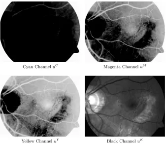
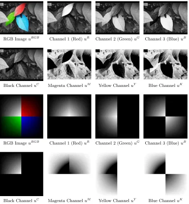
2.1 On the left, three bounded variation functions with the same total vari-ation. On the right, a function of no bounded varivari-ation. . . 14 2.2 Illustration of the RGB channels of a Colour Fundus retina image. Note
that much information can be seen in the green channel (c). . . 19 2.3 Two different views of the surface representation of the green channel of
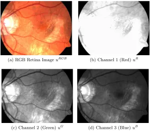
the Colour Fundus image given in Figure 2.2c. . . 20 2.4 Illustration of the CMYK channel representation of the Colour Fundus
retina image given in Figure 2.2a. . . 20 2.5 Illustration of the RGB and CYMK colour channels for two images.
From top to bottom, we show 1) Colour image and RGB channels of the Leaves image; 2) CMYK channels of the Leaves image; 3) Colour image and RGB Channels of the Colourball image; 4) CMYK channels of the Colourball image. . . 21 2.6 Illustration of (a) vertex-centred discretisation and (b) cell-centred
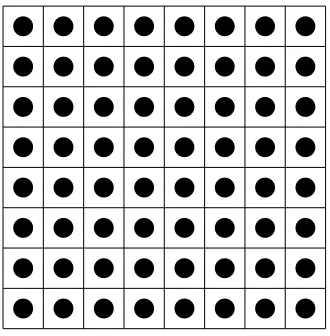
dis-cretisation of a square mesh. Red circles show the grid points. . . 22 2.7 Lexicographic ordering and Red-Black ordering for an 8×8 example.
On both rows, the figures on the left show Lexicographic ordering and the figures on the right show Red-Black ordering. . . 29
3.2 Example of the effect of adding Gaussian noise to give signal-to-noise ratio of 12. From left to right, we have (a) the noisy image, (b) the section of the noisy image outlined by the black square, (c) the intensity values of the noisy image along the yellow line (shown in green) compared with the intensity values of the clean, noiseless image along the same line (shown in blue). . . 48 3.3 Illustration of the performance of total variation denoising to restore
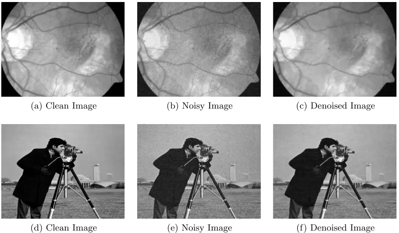
images from noise corruption. On the top row, we show an example of a Colour Fundus retina image (a) which has been corrupted by noise (b) with signal-to-noise-ratio (snr) of 28.1024 and restored using total variation (c) to snr 35.5171. On the bottom row, we show the camera-man example (a) which has been corrupted by noise (b) with snr of 28.1059 and restored using total variation (c) to snr 32.6741. . . 49 3.4 Illustration of the effect of blur on an image. From left to right, we have
(a) a Colour Fundus retina imageu, (b) the same imageu corrupted by out of focus blur, (c) the image u corrupted by Gaussian blur and (d) the imageu corrupted by linear motion blur. . . 51 3.5 Illustration of the performance of (3.15) with blurred data which is free
of noise. It can be noted that the restoration (b) of the image (a) with no additive noise by the minimisation (3.15) yields a very close approx-imation to the true solution. . . 54 3.6 Illustration of the performance of (3.15) with noisy data. The blurred
image (a) has been achieved by adding a small amount of noise to Figure 3.5a. It can be noted that, although the noise is visually imperceptible, the presence of noise means that the image cannot be restored (b) by the minimisation (3.15). . . 55 3.7 Illustration of the performance of (3.18) with noisy data. The noisy and
blurred image (a), which is the same as the image used in Figure 3.6a, has been restored (b) by the minimisation (3.18) withα = 10−3. It can be
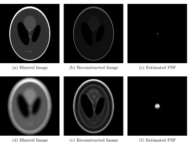
3.8 Illustration of the performance of Matlab’sdeconvblind command. On the top row, the “phantom” image of size 256×256 has been blurred with an out-of-focus blur function of diameter 3. On the bottom row, the same image has been blurred by an out-of-focus blur function of diameter 21. On both rows, from left to right we have (a, d) the blurred image, (b, e) the restored image and (c, f) the estimated blur function. In both cases, the blur function is approximately but not accurately estimated and the restored images contain many defects which are more obvious in the 2nd example (e). . . 71 3.9 Illustration of restoring multichannel images from blur corruption using
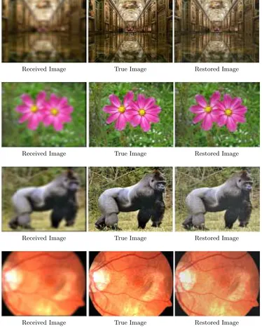
inter-channel information by solving the minimisation problem (3.55) with known point spread function. From top to bottom, we have the ex-amples 1) Apollo Gallery, 2) Aster, 3) Gorilla, 4) Colour Fundus Retina. On each row, from left to right, we have 1) the received data, 2) the true image which we want to approximate, 3) the restored image. In each case, the image is successfully restored and edges can be clearly seen. . . 73 3.10 Examples to demonstrate image segmentation. On the top row, we
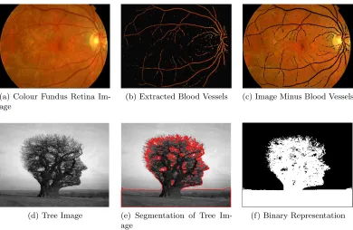
show retinal vessel segmentation of a Colour Fundus Angiography im-age. From left to right, we have the (a) image to be segmented, (b) the extracted blood vessels and (c) the image without the vessels which have been extracted. On the bottom row, we show the segmentation of the tree image (d). In image (e) we see that the tree and landscape can be separated from the sky by the red lines. Image (f) shows the binary representation of this segmentation, where white means foreground and black means background. . . 74
4.1 Real examples of image quality of Colour Fundus Images. . . 77 4.2 Real examples of image quality of Colour Fundus Images (Ch2). . . 77 4.3 Illustration of the deblurring of images by the total variation model
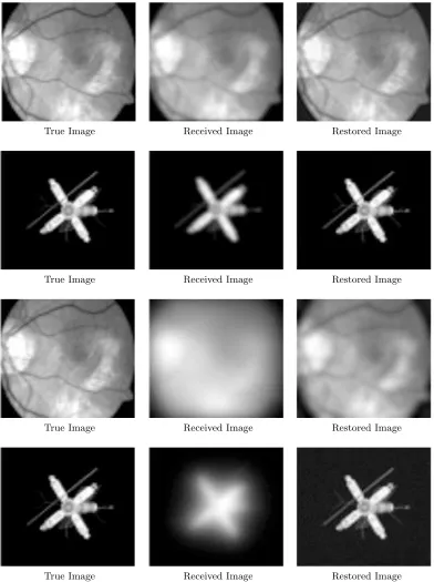
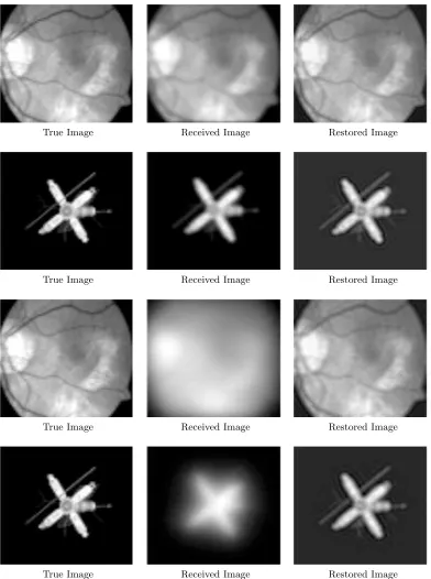
4.4 Illustration of the deblurring of images by the total variation model given Algorithm 8 assuming Neumann boundary conditions. From top to bottom, we have on each row examples of deblurring 1) a Fundus Autofluorescence retina image corrupted by motion blur, 2) a satellite image corrupted by motion blur, 3) a Fundus Autofluorescence retina image corrupted by Gaussian blur, and 4) a satellite image corrupted by Gaussian blur. On each row, from left to right, we have (1) the origi-nal (true) image, (2) the received (blurred) image, and (3) the restored (deblurred) image. . . 84 4.5 Illustration of the performance of Algorithm 9 with a colour Fundus
retina image, using Neumann boundary conditions. From left to right, we have (a) true image, (b) the received image and (c) the restored image. Some improvement can be seen in the restored image which has an improved SNR value (20.79) over the received image (19.15) and an improved PSNR value (27.00) of the received image (25.03). . . 87 4.6 Illustration of the performance of Algorithm 9 with the satellite image,
using Dirichlet boundary conditions. From left to right, we have (a) true image, (b) the received image and (c) the restored image. Some improvement can be seen in the restored image which has an improved SNR value (16.10) over the received image (8.95) and an improved PSNR value (30.23) of the received image (22.74). . . 88 4.7 Illustration of the performance of Algorithm 10 with a colour Fundus
Retina image corrupted by motion blur. On the left is (a) the received image and on the right (b) the restored image, obtained with a cpu time of 1.48. It can be noticed that the restored image with psnr 27.145 is an improvement on the received image (a) which has psnr 22.847. . . 93 4.8 Illustration of the performance of Algorithm 10 with a colour Fundus
Retina image corrupted by Gaussian blur. On the left is (a) the received image and on the right (b) the restored image, obtained with a cpu time of 1.63. It can be noticed that the restored image with psnr 27.003 is an improvement on the received image (a) which has psnr 17.862. . . 94 4.9 Illustration of the performance of Algorithm 10 with the satellite image
corrupted by motion blur. On the left is (a) the received image and on the right (b) the restored image. It can be noticed that the restored image with psnr 147.510 is an improvement on the received image (a) which has psnr 142.688. . . 95 4.10 Illustration of the performance of Algorithm 11 with the satellite image
4.11 Illustration of the performance of Algorithm 11 with the retina image corrupted by out of focus blur. The cpu time taken to obtain the restored image (b) given the received image (a) and to obtain the approximation of the blur function (d) from the initial estimate (c) is 18.77. . . 98 4.12 Illustration of the possible poor performance arising from solving the
minimisation problem (4.27) for the blurred satellite image. From left to right, we have (a) the received image of psnr 21.09, (b) the result after one iteration with psnr 15.19, (c) the result after 20 iterations with psnr 20.48. The psnr in both results is lower than that of the received image and the visual quality is clearly diminished. . . 99 4.13 Illustration of the results obtained after applying harsh constraints to
the image by simple projection onto the range [0, ζu] at each iteration
On the left is (a) the received image of psnr 21.09 and on the right (b) the approximated image of psnr 13.79. . . 100 4.14 Results of the blur function approximation obtained by solving the
min-imisation problem (4.27) with constraints. From left to right, we have (a) the true kernel we are aiming to approximate, (b) the approximated kernel using the constraints (4.28), and (c) the restored kernel using the constraints (4.28) as well as the image intensity based constraint. It can be noticed that as well as being imprecise there exists much noise in the approximation of the blur function. . . 101 4.15 Successful restoration of the blurred satellite image shown in Figure 4.12a
by Algorithm 12 withǫ= 1/3. On the left is (a) the approximated blur function and on the right (b) the restored image of psnr 27.28 which is an increase of 6.19dB compared to the received image. . . 103 4.16 Successful restoration of the blurred satellite image shown in Figure 4.12a
by Algorithm 12 withǫ= 10−2. On the left is (a) the approximated blur
function and on the right (b) the restored image of psnr 30.14 which is an increase of 9.05dB compared to the received image. . . 103 4.17 Successful restoration of the blurred retina image by Algorithm 12 with
ǫ= 10−2. The restored image (b) is a considerable improvement on the received image (a). . . 104 4.18 Illustration of the effect of intensity based constraints on a Gaussian
4.19 Illustration of the effect of location based constraints on a Gaussian function. From left to right, we have (a) the Gaussian function subject to intensity based constraint with ǫ= 10−2, (b) the Gaussian function
subject to location based constraint with δ = 15. The location based constraint allows the blur function to retain its structure while the in-tensity based constraint does not. . . 105 4.20 Restoration of the blurred satellite image by Algorithm 13. From left
to right, we have (a) the received image, (b) the restored image, (c) the approximated blur function. The restored image of psnr 24.71 shows visible improvement on the received image which has psnr 20.40. . . 107 4.21 Restoration of the blurred retina image by Algorithm 13. From left to
right, we have (a) the received image, (b) the restored image, (c) the approximated blur function. The restored image of psnr 30.38 shows visible improvement on the received image which has psnr 24.92. . . 107
5.1 Graph of Heaviside Transform u = T(ψ). On the left, we have (a) the transform ofψwith an exaggerateda4 and on the right (b) the projected
transform onto the range [τ1, τ2]. . . 112
5.2 Test case images. . . 124 5.3 PSFs used for test cases. Images (a)-(c) show Bl1 - small motion blur,
images (d)-(e) show Bl2 - large motion blur, images (f)-(h) show Bl3
-small Gaussian blur, and images (i)-(j) show Bl4 - large Gaussian blur. . 124
5.4 Result Set 1: Restoring Im1 corrupted by Bl3 with no noise. From top
to bottom, we have: 1) the true image, kernel, and corrupted data; 2) the result using the ROF method; 3) the result using Vogel’s method; 4) the result using the Transform method. From left to right, we have (on rows 2-4): 1) the restored image; 2) the negative values of the restored image in white; 3) the points where the intensity values are greater than the expected upper limit in white. Note that the Transform method and Vogel’s method can both ensure positivity but the transform method can control the upper bound of the intensity range. . . 128 5.5 Result Set 2 - restoring images Im2 and Im3 corrupted by small motion
blur Bl1 or small Gaussian blur Bl3. In some cases the results from
the Transform model appear sharper than other models and more small detail is visible. . . 129 5.6 Result Set 3 - Restoring Im2 corrupted by Bl2 (top line) and by Bl4
(bottom line). We can see a significant improvement in the result from the Transform method in the case of corruption by Bl2, and the results
5.7 Result Set 4 - Restoring Im2 corrupted by Bl3 and 1% noise (top row)
and 50% noise (bottom row). We can see that visually the Transform method appears to give improved results for weaker and stronger levels of noise. . . 132 5.8 Result Set 5: Restored images and PSFs using the Linearised Transform
method. The received data from which Im2 and Im3 were restored was
corrupted by Bl1, and the received data from which Bl1 and Bl3 were
restored was corrupted by Im2. We can see that the linearisation does
not affect the visual quality significantly. . . 133 5.9 Result Set 6: Restored images and PSFs using the Linearised Transform
method with the result of Vogel’s method as the initial estimate. . . 134 5.10 Result Set 7 - Restoring Bl1 (1st and 2nd rows) and Bl2 (3rd and 4th
rows) corrupted by Im1 restored using TV restoration (ROF), Vogel’s
model (Vogel) and the transform model (New15). In the cross-section images, the blue line is the restored image, the red dashed line is the lower bound of the true blur function and the green dashed line is the upper bound of the true blur function. Of the three approximations, as demonstrated in the cross-section images on the 2nd and 4th rows, the TV model gives many negative values in the approximation both kernels, and Vogel’s model has no negative values but struggles to get a close approximation while the transform model does a good job. . . 135 5.11 Graph of Transform u=T(ψ). On the left, (a) demonstrates the
corre-spondence between theσ andτ parameters and on the right, (b) shows that the differencesσ4−σ3 andτ4−τ3 are equal to Σ. . . 136
6.1 Good restoration results for Example 1 (box-triangle image): (b) from a corrupted image (a) using Algorithm 6. This model is able to improve the edges of the restored image (c), though the restoration is not excellent.142 6.2 Illustration of the failure of Algorithm 6 for a retinal scan (Example 2)
in (a): (b) corrupted image by motion blur; (c) failed restorationu; (d) restored u with thresholdingκ= 10−2; (e) restoredu with thresholding κ= 1/3; (f) restoredh with thresholdingκ= 1/3. . . 142 6.3 Test case images for experimental results. . . 160 6.4 Examples of blur functions used for experimental tests. In each case, we
have on image view of the blur function on the left and a mesh view of the same function on the right. . . 161 6.5 Row 1, l-r: Im1, received data corrupted by Bl1, restored image using
New16. Row 2, l-r: Im1, received data corrupted by Bl2, restored image
using New1
6. Our model is capable of restoring edges and preserving
6.6 Row 1, l-r: Im2, received data corrupted by Bl1, restored image using
New16. Row 2, l-r: Im2, received data corrupted by Bl2, restored image
using New1
6. Our model is capable of restoring details in both cases and
of preserving black space. . . 163 6.7 Row 1, l-r: Im3, received data corrupted by Bl1, restored image using
New1
6. Row 2, l-r: Im4, received data corrupted by Bl1, restored image
using New16. Our model is capable of restoring many detailed features and some fine details as well as sharpening edges. There are very few de-fects in the restored image, notably surrounding the rope in the restored Im4. . . 164
6.8 Row 1, l-r: Im3, received data corrupted by Bl2, restored image using
New1
6. Row 2, l-r: Im4, received data corrupted by Bl2, restored image
using New16. In the more challenging case of Gaussian blur, our model is capable of restoring some detailed features, including the books in the background of Im3 and the buildings in Im4. . . 165
6.9 Row 1, l-r: Im5, received data corrupted by Bl1, restored image using
New16. Row 2, l-r: Im6, received data corrupted by Bl1, restored image
using New1
6. Our model is capable of restoring many detailed features
and sharpen edges. Several of the blood vessels are made visible in Im5
and some very fine details can be distinguished in Im6. . . 166
6.10 Row 1, l-r: Im3, received data corrupted by Bl2, restored image using
New16. Row 2, l-r: Im4, received data corrupted by Bl2, restored image
using New16. Our model is capable of restoring some detailed features in these challenging cases. Much of the detail is restored in both cases. . . 167 6.11 (a) Im3 corrupted by Bl1, (b) restored image using New26, (c) Im3
cor-rupted by Bl2, (b) restored image using New26. Our accelerated model is
capable of obtaining good quality results. Much of the detail is restored in both cases. . . 167
7.1 Graphs of the integralf(σ) =RΩhO(x, y, σ) dΩ forn= 256 and varying σ. Note that while the integral appears to tend toward the unit for larger values ofσ, it is rarely equal to the unit for lower (more realistic) values. 179 7.2 Illustration of the Gauss Circle problem and the ability to preserve a
7.3 Illustration of the many local minima of the functionalF(σ) =||h(σ)∗u− z||2
2 againstσ for the Phantom image example with an out of focus blur
of radius 5.7: a) true imageu, b) true kernelh(x, y,5.7), c) received data z(x, y) =h(x, y,5.7)∗u(x, y), d)F(σ) appears to be convex however e) if we look closely near the global minimum there are many local minima resulting in f) many solutions to the minimisation problem. . . 181 7.4 Illustration of Parametric Blur functions. We have a) Out of Focus blur
hO(x, y, σ) with σ = 10, b) Box Blur hB(x, y, σ) with σ = 10, c) Linear Motion Blur hL(x, y, σ, θ) with σ = 10, θ = 0, d) Linear Motion Blur hL(x, y, σ, θ) withσ = 10, θ= 3π/4. . . 187 7.5 Images used for experimental testing. . . 189 7.6 Result Set 1: Illustration of the performance of Mod1, Mod4 and New17
with blurred images which have no additional noise. From left to right, we have 1) the received image z, 2) the restored image using Mod1, 3)
the restored image using Mod4, and 4) the restored image using New17.
All models show good results while the results of New17 appear to be sharper. . . 192 7.7 Result Set 2: Illustration of New7
7 for Im6. From left to right, we have
1) an example with no noise in the received image, 2) an example with noise to snr 30 in the received image, 3) an example with noise to snr 12 in the received image. From top to bottom: 1) Received image 2) Recovered blur function, 3) Recovered image. In the case of no noise, the blur function can be recovered, but in the cases of very small noise and larger noise the recovered parameters are too small leading to almost no reconstruction of the image or too large leading to over-deblurring of the image. . . 193 7.8 Result Set 3: Illustration of the performance of New2
7. On the top row,
the model unsuccessful identifies σ= 5.6 for the incorrect parameter α, on the bottom row, the model successfully identifiesσ= 5.2 as the min-imiser of F2 forα = 10−3. For this example, the correct reconstruction
appears to rely too heavily on the choice of parameter α. . . 194 7.9 Result Set 3: Illustration of the performance of Mod4, New17, New37 on
blurred images with noise. From left to right, we have 1) the received imagez, 2) the restored image using Mod4, 3) the restored image using
New1
7.10 Result Set 3: Illustration of the performance of New3
7 on noisy, blurred
images. From left to right, we have 1) Im5, 2) Im6, 3) Im4. From top
to bottom, we have 1) the received imagez, 2) the “denoised” image v and 3) the final deblurred image u. The separation of the noise from the image is successful and allows for the correct blur function to be identified and for the image to be deblurred. . . 196 7.11 Result Set 3: Illustration of the performance of Mod4, New17 and New37
on blurred images with greater noise. From left to right, we have 1) the received imagez, 2) the restored image using Mod4, 3) the restored
image using New17 and 4) the restored image using New37. . . 197 7.12 Result Sets 4 and 5: Illustration of the performance of New37 and New47
on images corrupted by out of focus blur. From left to right, we have 1) the received imagez, 2) the restored image using New37, 3) the restored image using New47. . . 198 7.13 Result Sets 4 and 5: Illustration of the performance of New3
7and New57on
images corrupted by box blur. From left to right, we have 1) the received imagez, 2) the restored image using New37, 3) the restored image using New5
7. . . 199
7.14 Result Sets 4 and 5: Illustration of the performance of New37and New67on images corrupted by box blur. From left to right, we have 1) the received imagez, 2) the restored image using New3
7, 3) the restored image using
New67. . . 200
8.1 Illustration of the continuous approximation ςε to the piecewise linear
functionς. For lower ε, the approximation is very close to ς. . . 207 8.2 Images used for test examples. . . 215 8.3 Segmentation of Images Im1–Im6 using model Mod1. . . 215
8.4 Illustration of the performance of the Mod1 for Im1 corrupted by
Gaus-sian blur: a) initial contour, b) segmentation given by Mod1, c,d)
seg-mentation given by New3
8. Mod1 gives a rough segmentation while the
spaces between the letters which are hidden by the blur are successfully segmented using New38. . . 219 8.5 Illustration of the performance of the New3
8 for Im2 corrupted by
Gaus-sian blur: a) received data, b,c) segmentation using New38, d) the dif-ference between the segmentation using New38 and using Mod1. The
segmentation is closer to the true edge using New3
8 while Mod1 also
cap-tures the blurred edge. . . 220 8.6 Result set 3. Illustration of the performance of New38 for (top-bottom)
Im4, Im3, Im5 and Im6 corrupted by Gaussian blur. The edges hidden
8.7 Result set 4. Illustration of the performance of the New3
8 for
(top-bottom) Im1, Im4, Im2 and Im6 corrupted by strong Gaussian blur.
New3
8 is capable of segmenting edges in these challenging cases which
cannot be segmented by Mod1. . . 223
8.8 Result set 5. Illustration of the performance of the New38 for (top-bottom) Im1, Im3, Im4 and Im5 corrupted by Gaussian blur and noise.
The edges hidden by blur are successfully segmented by New38 which cannot be segmented by Mod1. . . 226
List of Tables
4.1 Table of SNR and PSNR error values of images restored by Algorithm 7. The received retina and satellite images had been corrupted by motion and Gaussian blur. In each case, the algorithm is able to obtain an improved result. . . 80 4.2 Table of SNR and PSNR error values of images restored by Algorithms 7
and 8. The received retina and satellite images had been corrupted by motion and Gaussian blur. In each case, both algorithms are able to obtain improved results. In the case of the retina image, the case of Neumann boundary conditions provides an improved result. . . 83
5.1 Result Set 1 - Error values for Im1 corrupted by Gaussian blur with
no Noise. We can see that the error values are improved when using the Transform models and cpu time is improved by using New3
5–New75.
As designed, the results of New35–New75 are very similar, showing that the additional term does not have a considerable effect on results. It is also evident from New6
5–New75 that the final projection does not have a
significant impact on the results. . . 127 5.2 Result Set 2 - Error values for images Im2 and Im3 corrupted by Bl1.
It can be noticed that error values are improved using the Transform models. While cpu time is higher than that of competing models, New35– New7
5 can reduce cpu time while retaining similar or improved PSNR.
As designed, the results of New3
5–New75 are very similar, showing that
the additional term does not have a considerable effect on results. It is also evident from New6
5–New75 that the final projection does not have a
5.3 Result Set 2 - Error values for images Im2 and Im3 corrupted by Bl3.
It can be noticed that error values are improved using the Transform model. While cpu time is higher than that of competing models, New3
5–
New75 can reduce cpu time without a significant reduction in PSNR. As designed, the results of New35–New75 are very similar, showing that the additional term does not have a considerable effect on results. It is also evident from New65–New75 that the final projection does not have a significant impact on the results. . . 131 5.4 Result Set 3 - Error values for Im2 corrupted by Bl2 and Bl4. There is a
noticeable improvement in the case of and while the results for Bl4 are
competitive, the transform is slightly improved over competing models. 132 5.5 Result Set 4 - Error values for Im2corrupted by Bl2and varying amounts
of noise. We can see that the Transform model can offer improved results, particularly for larger levels of noise. . . 133 5.6 Result Set 5: Error values and cpu time for restoring images Im2 and
Im3 as well as PSFs Bl1 and Bl3 using the Transform method and the
Linearised Transform method. We can see that the quality of the restored image is not significantly different for each case but the cpu time is improved using the Linearised Transform method. . . 133 5.7 Result Set 6: Error values and cpu times for restoring images Im2 and
Im3 and PSFs Bl1 and Bl3 using the Linearised Transform method with
the received data z as the initial estimate (New15) and the result from Vogel’s method as the initial estimate (New55). The cpu time is rarely lower when using the closer initial estimate but the image quality is improved in all cases. . . 134
7.1 Error values for images Im1-Im3 corrupted by Bl1 and a small amount
of additive noise, restored by models Mod1-Mod6, New17, New37. . . 191
7.2 Error values for images Im4-Im6 corrupted by Bl1 and a small amount
of additive noise, restored by models Mod1-Mod6, New17, New37. . . 191
7.3 Error values for images Im1-Im3 corrupted by Bl1 and additive noise,
restored by models Mod1-Mod6, New17, New37. . . 193
7.4 Error values for images Im4-Im6 corrupted by Bl1 and additive noise,
restored by models Mod1-Mod6, New17, New37. . . 194
8.1 Result set 1. Error values for Im1–Im6 corrupted by Gaussian blur and
segmented by Mod1. . . 218
8.2 Result set 2. Error values for Im1–Im6 corrupted by Gaussian blur and
segmented by Mod3 and New28. The competition is close for most
exam-ples, but overall New2
8.3 Result sets 3,6. Error values and cpu times for images Im1–Im4
cor-rupted by small Gaussian blur. Error values are improved with New38 and New4
8. New38 achieves better error values with the exception of
con-tour length which is closer with or identical to the result from New48 while New48 achieves the lowest cpu time. For Im1, the cpu time is lower
for Mod1, but the error values are considerably deteriorated. . . 220
8.4 Result sets 3,6. Error values and cpu times for Im5, Im6, ‘Circles’ and
‘Knee’ images corrupted by small Gaussian blur. In all cases, New38 and New4
8 achieve improved results. The contour length is typically closer
with New48 and while for most examples the cpu time is lower for Mod1,
it is closely followed by New48 which gives considerably better results. . . 222 8.5 Result sets 4,6. Error values and cpu times for images Im1–Im4
cor-rupted by strong Gaussian blur. In all cases, New38 and New48 achieve improved results although the contour length of the results from Mod4
is better for Im3. For most cases, the cpu time is lower for New48 with
the exception of Im1 which has slightly lower cpu time for Mod1 with
deteriorated results. . . 224 8.6 Result sets 4,6. Error values and cpu times for Im5, Im6, ‘Circles’ and
‘Knee’ images corrupted by strong Gaussian blur. In all cases, New38and New48 achieve improved results and competition is close between New38 and New4
8. Cpu time is lower for New48in two cases,. It is lower for Mod1
is two other cases followed by New48 which achieved considerably better results. . . 225 8.7 Result sets 5,6. Error values and cpu times for Im1, Im3–Im5 corrupted
by Gaussian blur and noise. In all cases, New38 and New48 achieve im-proved results with the exception that the contour length is of the result for Im4 was closer to the true contour with Mod1. Cpu time is lower
for New48 in two cases. In the remaining cases, it is lower for Mod1 and
closely followed by New4
8 which achieved significantly improved results. . 227
8.8 Result set 7. Error values given byEr1 for Im1–Im4 corrupted by
Gaus-sian blur and segmented by New18, New38 and New48. For Im1, New18
out-performs the other models but in the remaining cases New3
8 and New48
List of Algorithms
1 Jacobi Method (JAC) . . . 26 2 Gauss-Seidel Method (GS) . . . 28 3 Newton’s Method (NEWT) . . . 33 4 Conjugate Gradient Method (CG) . . . 38 5 Preconditioned Conjugate Gradient Method (PCG) . . . 39 6 Chan-Wong [54] Method (CW) . . . 68 7 TV Deblurring with Dirichlet Boundary Conditions (TVDD) . . . 80 8 TV Deblurring with Neumann Boundary Conditions (TVDN) . . . 82 9 Blind TV Deblurring (BTVD) . . . 87 10 Split Variable Deblurring (SVaD) . . . 92 11 Blind Split Variable Deblurring (BSVaD) . . . 96 12 Deblurring with Local Support Kernels (DLSK) . . . 102 13 Deblurring with Global Support Kernels (DGSK) . . . 106 14 A Transform Based Constrained Deblurring Algorithm (TCD) . . . 114 15 Accelerated Transform Based Constrained Deblurring (ATCD) . . . 118 16 Convex Transform based Implicitly Constrained Deblurring (CTCD) . . 120 17 The First Transform Method (TM1) for Model (6.7) via (6.9) and (6.10). 148 18 The Second Constrained Transform Based Algorithm with ADM (TM2) 157 19 Constrained Parametric Deblurring (CPD1) . . . 175 20 Constrained Parametric Deblurring (CPD2) . . . 177 21 Segmentation of Blurred Images (wsc1) . . . 208
22 Segmentation of Blurred Images (wsc2) . . . 209
23 Segmentation of blurred images (wsc3) . . . 211
Publications
Mathematical Methods and Algorithms for Restoring Retinal Images with Blur and Blind Blur. Bryan M. Williams, Ke Chen, Yalin Zheng and Simon P. Hard-ing. Ophthalmology Image Analysis Workshop, University of Liverpool. December 02, 2011.
Advanced Blur Removal Methods with Applications to Retinal Imaging for Ophthalmology. Bryan M. Williams, Ke Chen, Yalin Zheng and Simon P. Harding. Medical Image Understanding and Analysis 2012. 286–291. 2012.
A New Constrained Total Variational Deblurring Model and Its Fast Algo-rithm. Bryan M. Williams, Simon P. Harding and Ke Chen. Numerical Algorithms. To appear. 2014.
A New Study of Blind Deconvolution with Implicit Incorporation of Non-negativity Constraints. Bryan M. Williams, Ke Chen, Yalin Zheng and Simon P. Harding. International Journal of Computational Mathematics. To appear. 2014.
An Effective Variational Model for Simultaneous Reconstruction and Seg-mentation of Blurred Images. Bryan M. Williams, Jack A. Spencer, Ke Chen, Yalin Zheng and Simon P. Harding. Computer Vision Image and Understanding Special Issue on Discrete and Continuous Geometry in Computer Vision. Submitted. 2014.
An Enhanced Model for Semi-Blind Deblurring with Parametric Kernel Identification and Constrained Image Reconstruction. Bryan M. Williams, Ke Chen, Yalin Zheng and Simon P. Harding. In Preparation. 2014.
Presentations
Mathematical Methods and Algorithms for Restoring Retinal Images with Blur and Blind Blur.
Bryan M. Williams. Ophthalmic Image Analysis Workshop, University of Liverpool. December 02, 2011.
Mathematical Methods for Blind Image Deblurring.
A Blind Deconvolution Model for Images Corrupted by Gaussian Blur. Bryan M. Williams. Essex-Greenwich-Hertfordshire Workshop on Applied and Numer-ical Mathematics - Multiscale Problems, University of Greenwich. June 07–08, 2012.
Advanced Blur Removal Methods with Applications to Retinal Imaging for Ophthalmology.
Bryan M. Williams. 16th Conference on Medical Image Understanding and Analysis, Swansea University. July 09–11, 2012.
Advanced Mathematical Methods for Medical Image Enhancement.
Bryan M. Williams. Workshop on Ageing, University of Liverpool. December 19, 2012.
Mathematical Deblurring of Images for Non-Blind and Blind Restoration. Bryan M. Williams. 25th Biennial Numerical Analysis Conference, University of Strath-clyde. June 24–28, 2013.
Image Deconvolution Techniques.
Chapter 1
Introduction
This thesis is about developing mathematical models for image restoration, particularly in image deblurring.
In this chapter, we present an introduction to deblurring as an image processing technique in §1.1 along with a brief overview of how the problem of blur degradation can be modelled and the different classes of image deblurring problems encountered. We also present in§1.2 an outline of the chapters of this thesis.
1.1
Introduction to Image Deblurring
Image processing incorporates many problems such as image reconstruction which includes removing image noise from a given image by denoising [26, 28, 56, 169], the task of reconstructing an image from a given blurred image known as deblurring [54, 123, 177, 104, 2, 208, 210] and reconstructing a missing or damaged portion of an image (inpainting) [6, 16, 25, 52]. Other important image processing techniques include emphasising the boundaries of an image by different filters or segmenting an image into subregions [8, 12, 53, 69, 162] andregistration which attempts to align two images based on some measure of similarity [171, 139, 140, 106, 110, 189, 77] as well as others [107, 130, 146, 73, 217, 80, 128, 159, 101, 158, 175].
A significant problem in image processing isimage deblurringordeconvolution. This is the process of restoring a hidden true image from a given blurred image enabling edges to be sharper, hidden features to be revealed and details to be clearly visible. In this section we introduce the issue of blur in images and the task of restoring an image from blur degradation.
1.1.1 The Problem of Blur Degradation of Images
Blurring of images occurs in many fields such as astronomical imaging, remote sens-ing, microscopy and medical imaging such as Colour Fundus Angiography for retinal imaging, which is our main interest.
diffi-cult to obtain yet vital for diagnosis and screening as well as further processing such as registration. It is particularly important to get as much information as possible of retinal vessels and other structures for treatment and management as well as for grad-ing. Some examples of retinal scans which vary in quality from excellent to inadequate are shown in Figure 1.1.
Excellent Good Fair Inadequate
Figure 1.1: Examples of Colour Fundus images of varying quality fromexcellent where blood vessels and other details can clearly be seen to inadequate where most of the detail is not visible. Such inadequate images cannot be used for diagnosis or screening.
Blurring in retinal images leads to a substantial number of unnecessary referrals and in turn a waste of valuable hospital resource. In a current programme which sees three million diabetic patients undergo annual photographic screening, approximately 10% of the images acquired (by high-resolution digital cameras) are considered to be too blurred for assessment and so ungradeable due to inadequate clarity or poor field definition. This proportion of inadequate scans is typical of retinal imaging and may result in further referrals or even misdiagnosis. Such visually ungradeable images are more likely to come from patients who have reached an advanced stage of Retinopathy. Blurring of images is due to many factors such as motion of the camera or the tar-get scene, defocusing of the lens system, imperfections in the electronic, photographic, transmission medium, and obstructions. In retinal imaging, there are many contribut-ing factors influenccontribut-ing the quality of the received scan includcontribut-ing patient-related factors such as eye movement and the age of the patient. Those who are particularly young or old find it difficult to keep the eye still during the process, making it difficult to obtain an adequate scan. Advanced ocular diseases and other coexisting conditions such as Parkinson’s disease also make it difficult for light to pass through the eye and can cause blur. Refractive error, difficulty maintaining careful focus and the skill and experience of the photographer are also contributing factors.
1.1.2 Modelling the Blurring Process
An observed blurred image can be written as a convolution of the true image with a linear shift-invariant (lsi) blur, known as the point spread function (psf) or unknown kernel functionκ(x, y) [117].
In order to model the blurring of an imageu(x, y), we discretise the image function over an nx×ny pixel mesh. Letting z(x, y) denote the received (corrupted) image,
collection of data andu(x, y) denote the hidden true image which we wish to recover, we model the blurred imagez(x, y) as
z(x, y) = [κ∗u](x, y) +η(x, y)
where∗ denotes the operation of convolution which is given by
[κ∗u](x, y) =
Z ∞
−∞
Z ∞
−∞
κ(x−x′, y−y′)u(x′, y′) dx′dy′
for the convolution of the kernelκ(x, y) and the true imageu(x, y). See Figure 1.2 for an example of forming a blurred and noisy image from a sharp, clean image.
(a) True Imageu(x) (b) Blur Functionκ(x) (c) Noise Functionη(x) (d) Blurred Imagez(x)
Figure 1.2: Illustration of the blurring process. From left to right we have (a) the true image u(x), (b) the blur function κ(x), (c) the additive noise acquired η(x), and (d) the received imagez(x) = [κ∗u](x) +η(x).
1.1.3 Restoring Images from Blur Degradation
Attempting to recover the lost true image u(x, y) typically leads to solving the large system
Au=b where b=K⊤z, A=K⊤K+αL,
whereK is an ill-conditioned (typically full) matrix, z is the received corrupted data, Lis a sparse regularisation matrix which may or may not be symmetric, andαis scalar quantity known as the regularisation parameter, usually small and positive, which is used to control the amount of regularisation.
There are three main deconvolution problems:
1. Deconvolution in the case of known blur, known asnon-blind deconvolution, has been investigated widely in the last few decades giving rise to a variety of solutions [119, 178, 11, 207, 13, 94, 104, 193]. In this case, the point spread function is assumed known even though this information is not available in most of the real applications. The challenge is to recover the true image.
as a Gaussian function. The task then is to recover the image and estimate the correct parameters which identify the blur.
3. Blind image deconvolution includes the cases where both the blur kernel and the image are unknown [216, 117, 118, 54, 55, 141, 2, 31, 64, 78, 103, 126]. In these cases, the problem becomes harder and much more challenging since both the blur function and true image must be found, but it has much greater applicability to real-world problems.
Each of the above types of deblurring problem is important in many scientific appli-cations such as astronomical imaging, medical imaging, and remote sensing as well as consumer photography.
1.2
Thesis Outline
The remaining chapters of this thesis are organised as follows.
Chapter 2 - Mathematical Preliminaries
In this chapter, we present some mathematical tools which will be used throughout this thesis which the reader may wish to review while reading subsequent chapters. A brief review will be given with definitions, theorems and examples of some important relevant mathematical topics including linear spaces, variations of a functional, bounded space of variation, inverse problems and image representation. The discretisation of partial differential equations using finite differences and iterative solutions of linear and non-linear equations are also presented. An overview of some relevant numerical methods such as Newton’s method and the Steepest Descent method will be given as well as some fast solver algorithms including Conjugate Gradient.
Chapter 3 - Review of Variational Models for Image Reconstruction
In this chapter, we present a brief revision of some variational models for image restora-tion and reconstrucrestora-tion techniques. We begin with an introducrestora-tion to noise corruprestora-tion in images and denoising techniques using filters such as the total variation (tv) regu-larisation functional based on the Rudin-Osher-Fatemi (ROF) denoising model, intro-ducing some its properties and covering the benefits and drawbacks before discussing alternative forms of regularisation. We then introduce the problem of blur corruption in images in more detail and introduce some deconvolution techniques in the non-blind, semi-blind and blind cases. We also present some work in image segmentation which may be useful when reading Chapter 8.
Chapter 4 - Application to Blurred Images and some Refinements
to minimise the functional and discuss the methods of solving such equations accu-rately and efficiently. We then present some refinements to these models. We consider an enhancement of such models achieved by varying the boundary conditions in the cases of blind and non-blind deconvolution and a fixed-point method for solving the resulting system quickly, presenting experimental results. We next present a method for obtaining a fast solution to the deblurring problem by variable splitting, separating a dense and non-linear system into two systems which may each be solved efficiently. Finally, we present a method which aims to improve blur function estimation in the case of blind deblurring by imposing filtering on the kernel function and considering methods of regularisation depending on assumption of the blur type.
Chapter 5 - A New Constrained Deblurring Model
In this chapter we consider techniques for preserving non-negativity and in particular the intensity range in image deblurring and discuss the introduction of non-negativity constraints both explicitly and implicitly. Beginning with a constrained model, we develop an unconstrained model which is able to successfully preserve the range of intensity values of an image when it is reconstructed from a corrupt image using known information about the blurring function. We consider alternative regularisation and two forms of the constrained model given by linearisation and by alternate direction methods. We then discuss convexity of the model, introducing a convex variant of the functional. Numerical evidence showing the quality of reconstruction is presented.
Chapter 6 - A Robust Model for Constrained Blind Image Deblurring
In this chapter, we review some methods for solving the constrained blind deconvo-lution problem and the issues of imposing such artificial constraints and of relaxing them. By imposing such constraints, we may not minimise the given function, but by not imposing the non-negativity constraint or the upper-value constraint, we risk converging towards a false solution. We present an adaptation of the implicitly con-strained deblurring model for use when identifying the cause of the blur corruption. In this case, we assume that the blur function satisfies a non-negativity constraint. We present a model to impose this constraint implicitly and a strategy for dealing with the non-linearity and recovering the image and blurring kernel simultaneously. We next present a modification of this method which is able to obtain a fast result and incorporates alternative regularisation for smooth blur functions. Finally, we present experimental results demonstrating the effectiveness of this work.
Chapter 7 - Semi-Blind Deblurring with Parametric Kernel Identification
focus. We present a parametric deblurring model for images corrupted by Gaussian blur which may be modelled using a well-known formulation. We next present three enhancements to this model by implicitly constraining the range of the image intensity values, considering regularisation of the blur function and separation of the image noise in the energy functional. We then present formulations for alternative blur types (out of focus, linear motion and box blurs) which are able to well approximate these piecewise-constant blur functions. These formulations are continuous but give a very close approximation to the blur kernels such that the difference error, particularly after discretisation, is extremely small. We thus present models which incorporate the new formulation of these blur functions in the functional with experimental results.
Chapter 8 - Simultaneous Reconstruction and Segmentation of Blurred Im-ages
In this chapter, we introduce an application of image deblurring to a method for seg-menting blurred images. We present a review of some existing work in this area and a model for segmenting images which have been corrupted by blur and Poisson noise in a two-stage framework which involves first approximating the sharp image and then applying a segmentation technique to the result which aims to find the global minimum of the segmentation problem, which is typically non-convex. We then introduce a new joint model which aims to simultaneously segment the image as it is restored from blur degradation, followed by an accelerated model which uses alternate direction methods to connect the problems of segmentation and deblurring in order to form a joint energy functional. We present some relevant measures of error, including four novel measures and experimental results which demonstrate the effectiveness of this work.
Chapter 9 - Conclusions and Future Research
Chapter 2
Mathematical Preliminaries
In this chapter, we present some mathematical theory which may be useful to the reader throughout this thesis. We begin with an introduction to normed linear spaces with some useful examples and present some relevant theory about calculus of variation. Next, we discuss inverse problems and regularisation before moving on to image repre-sentation and discretisation, finishing with an introduction to some iterative methods for solving partial differential equations.
2.1
Normed Linear Spaces
In order to extend working on the real lineRton-dimensional Euclidean spaceRn, we require some structure. This leads to the class of normed linear spaces.
We first introduce some relevant notation and definitions which will be useful throughout this thesis and which may found in literature relating to advanced calculus and linear algebra.
We represent the elementsx∈Rnof then-dimensional Euclidean space byn-tuples (x1, . . . , xn), called vectors or points inRnwhich for brevity we will usually denote with
a bold character, such as
x = (x1, . . . , xn) ∈ Rn. (2.1)
The structures of the inner product or dot product of two vectors x,y ∈ Rn is defined as
x·y = hx,yi = x1y1+· · ·+xnyn, (2.2)
and thelength of a vector as
kxk = √x·x = qx2
1+· · ·+x2n, (2.3)
Definition 2.1.1 (Norm). Let N :L⊆Rn → R be a real valued function. Then N is called a norm on L if it satisfies the following properties for all x,y∈L:
• N(x) = 0 ⇒ x = 0,
• Absolute homogeneity: N(αx) =|α|N(x) ∀α∈R,
• Triangle inequality: N(x+y) ≤ N(x) +N(y). The norm of a vector x is commonly represented bykxk.
Remark 2.1.2 By the absolute homogeneity axiom, we have N(−x) =N(x) so that by the triangle inequality, we have positivity, i.e. N(x)≥0.
Remark 2.1.3 The definition of a seminormis the same as that of a norm but without the first axiom.
Some examples of functions which are norms are given below.
Example 2.1.4 (p-norm). Let x∈ Rn, then for any p∈ R≥1 we define the p-norm of x as
kxkp =
n
X
i=1
|xi|p
!1/p
. (2.4)
Note that the Euclidean norm given above in Equation (2.3) can be achieved by setting p= 2 in (2.4).
Example 2.1.5 (Lp-norm). Let f be a function defined on a domain Ω and 1≤p≤ ∞. We define the Lp-norm off onΩ as
kf(x)kp =
Z
Ω|
f(x)|p dx
1/p
. (2.5)
Note that since f may have arbitrarily many components, this is a generalisation of Example 2.1.4.
Example 2.1.6 (L∞-norm). The special case of the Lp-norm from Example 2.1.5 where p=∞ is defined as
kf(x)k∞= sup
x |f(x)|. (2.6)
We may now define the concepts of linear spaces and in particular normed linear linear spaces.
Definition 2.1.7 (Linear space). Let L= (P, K, I) be an incidence structure. That is, a triple whereP is a set of points,L is a set of lines andI ⊆P×K is an incidence relation such that if (p, l)∈I then we consider the pointp to lie on the line l. Then L is a linear space if
• Two points are incident with exactly one line. That is, ifp1, p2∈P andl1, l2 ∈K
are distinct points and lines such that
{(p1, l1),(p2, l1),(p1, l2),(p2, l2)} ⊆I
• Each line is incident with at least two points. That is, for all l∈ K there exist distinctp1, p2 ∈P such that(p1, l)∈I and (p2, l)∈I.
Definition 2.1.8 (Normed linear space). A normed linear space is a pair (L, N) where L is a linear space andN is a norm defined on L.
Definition 2.1.9 (Cauchy sequence). Let {xi} be a sequence in the space L. We say that this is a Cauchy sequence if for every ε∈R>0 there exists M ∈Z+ such that for every natural number m, n > M, we havekxm−xnk< ε.
Definition 2.1.10 (Banach space). A normed linear space L is called a Banach Spaceif it is complete. That is, if every Cauchy sequence in Lconverges to an element in L.
Remark 2.1.11 For an example of a Banach space, we may take any Hilbert space, defined as an inner product space which is also a metric space with respect to the distance function induced by the inner product. Euclidean space is an example of a Hilbert space.
2.1.1 Convex Functions
Here, we introduce the idea of convex functions and present some examples.
Definition 2.1.12 (Linear transformation). A function T : L → M is called a linear transformationif, for any x,y∈L and any α∈R, we have
1. T(x+y) =T(x) +T(y), 2. T(αx) =αT(x).
Definition 2.1.13 (Convex function). Let Sbe a convex subset of ann-dimensional vector space V, that is for any r >1 vectors x1, . . . ,xr ∈S and any λ1, . . . , λr ∈R≥0
such thatλ1+. . .+λr = 1 we have λ1x1+. . .+λrxr∈S. Then a functionf defined
onS is called convex if for all xi,xj ∈S and α∈(0,1) we have
f(αxi+ (1−α)xj)≤αf(xi) + (1−α)f(xj). (2.7)
f is called strictly convex if the inequality is strict for xi 6=xj.
Remark 2.1.14 There are several operations which preserve convexity:
• Weighted sums: Let f and g be convex functions on Rn. Then the linear combi-nationh=αf+βg is also convex for α, β≥0.
• Affine substitutions of the argument: Let f be a convex function on Rn and P : Rm → Rn be an affine mapping given by P(x) =Ax+b. Then f(P(x)) is also convex.
• Pointwise sup: Letfα define a family of convex functions on Rn. Then the upper
bound supαfα is convex.
1. A function f which is differentiable everywhere onA is convex on A if and only if its derivative is monotonically non-decreasing on A.
2. A functionf which is twice differentiable everywhere onA is convex onA if and only if its second derivative is non-negative on A.
Example 2.1.16 Let u: Ω⊆R2 →R and define the total variation T V(u) of u as
T V(u) =
Z
Ω|∇
u|.1
We show that the total variation is a convex function as follows. Let u1 6=u2 be two
functions. Then
T V(αu1+ (1−α)u2) =
Z
Ω|∇
(αu1+ (1−α)u2)|=
Z
Ω|
α∇u1+ (1−α)∇u2|
≤α
Z
Ω|∇
u1|+ (1−α)
Z
Ω|∇
u2|=αT V(u1) + (1−α)T V(u2).
Example 2.1.17 The square of theL2-norm of a functionu: Ω⊆R→R given by
kuk22 =
Z
Ω|
u|2dx
is convex. We show this as follows. Introducing a functionφ and parameterε, we can calculate the second derivative of a functionF(u) by making the substitutionv=u+εφ and finding the second derivative with respect to εas follows:
d2F(v) dε2 =
d dε dF(v) dv dv dε = d dε dF(v) dv φ = d
2F(v)
dv2
dv dεφ=
d2F(v) dv2 φ
2.
Applying this idea to the L2-norm, we have d2
dε2ku+εφk 2 2 =
Z
Ω
d2
dε2(u+εφ)
2dx=Z Ω
d
dε2(u+εφ)φdx= 2
Z
Ω
φ2dx
and so the second derivative is non-negative. Then by Theorem 2.1.15, the square of the L2-norm of the function u is convex.
Note also that by Remark 2.1.14, the square of theL2-norm of a linear combination of functions given by
ku+λvk22 =
Z
Ω|
u+λv|2dx
is also convex for functions u, v: Ω⊆R→R and λ∈R.
2.1.2 Differentiable Functions
We would now like to generalise the idea of a derivative of a real-valued function of a single variable to the case of a vector valued function of multiple variables. The Fr´echet derivative generalises this idea to functions on Banach spaces.
1Note that the total variationR
Ω|∇u(x)|is commonly written as
R
Definition 2.1.18 (Fr´echet derivative). Let f : U → W be a function defined on an open subsetU ⊆Lof a Banach spaceL, taking values in a second Banach spaceW. Then we say that f is Fr´echet differentiable at x∈ U if there exists a bounded linear operatorTx:L→W such that
lim
h→0
kf(x+h)−f(x)−Tx(h)kW
khkL = 0.
We then call f′(x) =Tx the Fr´echet derivative of f at x.
In contrast, the Gˆateau derivative generalises the idea of the directional derivative.
Definition 2.1.19 (Gˆateux derivative). Let f be a function defined on an open subset U ⊆L of a Banach space L, taking values in a second Banach space W. Then we say that f :U → W is Gˆateau differentiable at x∈ U if the two-sided directional derivative f′(x0;v) exists for each v ∈L; that is, if there exists g:V →W such that
g(v) = lim
ε→0
f(x+εv)−f(x)
ε . (2.8)
Remark 2.1.20 Note that if the Fr´echet derivative off exists atx, thenf is Gˆateaux differentiable at x and the two derivatives coincide but the opposite does not hold.
2.2
Calculus of Variations
We now introduce the basic theory which we require in order to derive the first variation or Euler-Lagrange equation of a functional. The reader may wish to consult sources such as [81, 83, 84] for more information.
We begin by introducing the first variation of a functional and a necessary condition to be satisfied by a minimiser of a variational integral. We then present the Divergence theorem, leading to integration by parts and some relevant examples of finding the first variation of a functional.
2.2.1 Variation of a Functional
Let
J[u] =
Z
Ω
F(x, u(x),∇u(x)) dx (2.9)
be a functional which is defined on some normed linear space and dependent on an independent variablex= (x1, x2, . . . , xn), an unknown functionu(x), and its gradient
given by ∇u(x) = (u(x)x1, u(x)x2, . . . , u(x)xn). Here dx is the n-differential element defined as dx= dx1dx2· · ·dxn.
The most important necessary condition to be satisfied by any minimiser of a vari-ational integral likeJ(u) is the vanishing of its first variation δJ defined as
δJ(u) = d
dεJ(u+εϕ)
ε=0
This is, if u is a minimiser of J(u) with respect to variations δu = ϕ which do not change boundary values ofu, then (2.10) must be satisfied for all ϕwith compact support2 in Ω. Then for some u
0 ∈Ω, we callδJ(u0) the first variation ofJ atu0 in
the direction ofϕ.
To compute the first variation of variational integrals like (2.9) on the direction of a function ϕ(x) with compact support in Ω, we define the following transformation:
u∗(x) =u(x) +εϕ(x) +O(ε2), (2.11)
whereε→0 and kϕk →0. Then the variationδJ of the functional (2.9) corresponding to the above transformation is defined as the linear part inεof the differenceJ[u∗]−J[u]. Using Taylor’s theorem, it is possible to show (see for example [81]) that
J[u∗]−J[u] =ε
Z
Ω
Fu+ n
X
i=1
Fuxiϕxi
!
dx+O(ε2). (2.12)
It follows then that the variation of the functional (2.9) is given by
δJ =
Z
Ω
Fu+ n
X
i=1
Fuxiϕxi
!
dx. (2.13)
2.2.2 The Divergence Theorem and Integration by Parts
Consider an open and bounded subset Ω⊂Rn with piece-wise smooth boundary ∂Ω. Suppose a scalar functionu(x) is continuously differentiable on ¯Ω. Then
Z
Ω
uxidx=
Z
∂Ω
u(x)νids (2.14)
is satisfied for i = 1, . . . , n with ν = (ν1, ν2, . . . , νn) the outward unit normal of ∂Ω.
Using this result and simple additivity, it is simple to show that for a given vector field
F =F(x) the following is true
Z
Ω
(∇ ·F) dx=
Z
∂Ω
F ·ν ds. (2.15)
The latter is the most common way to present the divergence theorem.
An immediate consequence of the divergence theorem is the integration by parts formula. This is, fori= 1, . . . , nand for two continuously differentiable functionsu(x) and v(x) in ¯Ω
Z
Ω
uxiv(x) dx=−
Z
Ω
u(x)vxi dx+
Z
∂Ω
u(x)v(x)νids. (2.16)
Additionally, by applying (2.15) to the product of a scalar function g and a vector
2The support of a function is the set of points where this function is not zero. Functions with