Sensor Fusion and Deep Learning for Indoor Agent Localization

Theses Thesis/Dissertation Collections

6-2017

Sensor Fusion and Deep Learning for Indoor

Agent Localization

Jacob F. Lauzon

Follow this and additional works at:http://scholarworks.rit.edu/theses

This Thesis is brought to you for free and open access by the Thesis/Dissertation Collections at RIT Scholar Works. It has been accepted for inclusion in Theses by an authorized administrator of RIT Scholar Works. For more information, please [email protected].

Recommended Citation

for Indoor Agent Localization

By

Jacob F. Lauzon

June 2017

A Thesis Submitted in Partial Fulfillment of the Requirements for the Degree of Master of Science

in Computer Engineering

Approved by:

Dr. Raymond Ptucha, Assistant Professor Date

Thesis Advisor, Department of Computer Engineering

Dr. Roy Melton, Principal Lecturer Date

Committee Member, Department of Computer Engineering

Dr. Andres Kwasinski, Associate Professor Date

Committee Member, Department of Computer Engineering

Firstly, I would like to sincerely thank my advisor Dr. Raymond Ptucha for his

unrelenting support throughout the entire process and for always pushing me to

better my work and myself. Without him, and his mentorship, none of this would

have been possible.

I would also like to thank my committee, Dr. Roy Melton and Dr. Andres

Kwasinski for their added support and flexibility.

I also must thank the amazing team of people that I have worked with on the

Milpet project, both past and present, that has dedicated many long hours to making

the project a success. In particular I would like to thank Rasika Kangutkar for her

work on ROS, path planning, and obstacle avoidance, Alexander Synesael for his work

on the hardware systems, and Nicholas Jenis for his work on the mobile applications.

Autonomous, self-navigating agents have been rising in popularity due to a push for

a more technologically aided future. From cars to vacuum cleaners, the applications

of self-navigating agents are vast and span many different fields and aspects of life.

As the demand for these autonomous robotic agents has been increasing, so has

the demand for innovative features, robust behavior, and lower cost hardware. One

particular area with a constant demand for improvement is localization, or an agent’s

ability to determine where it is located within its environment. Whether the agent’s

environment is primarily indoor or outdoor, dense or sparse, static or dynamic, an

agent must be able to have knowledge of its location. Many different techniques

exist today for localization, each having its strengths and weaknesses. Despite the

abundance of different techniques, there is still room for improvement. This research

presents a novel indoor localization algorithm that fuses data from multiple sensors

for a relatively low cost. Inspired by recent innovations in deep learning and particle

filters, a fast, robust, and accurate autonomous localization system has been created.

Results demonstrate that the proposed system is both real-time and robust against

Acknowledgments i

Abstract ii

Table of Contents iii

List of Figures v

List of Tables viii

Acronyms ix

1 Introduction 2

2 Background 6

2.1 Localization . . . 6

2.1.1 Dead Reckoning . . . 7

2.1.2 Signal-Based Localization . . . 8

2.1.3 Sensor Networks . . . 8

2.1.4 Vision-Based Localization . . . 9

2.2 Filtering . . . 12

2.2.1 Kalman Filters . . . 12

2.2.2 Particle Filters . . . 15

2.3 Support Vector Machines . . . 18

2.4 Deep Learning . . . 21

2.4.1 Convolutional Neural Networks . . . 22

2.5 Deep Residual Networks . . . 31

3 Platform 36 3.1 Hardware . . . 36

3.2 Software . . . 47

3.2.1 Embedded PC . . . 48

3.2.2 Microcontroller . . . 55

4 Methods 65

4.1 Overview . . . 65

4.2 Testing Environment . . . 65

4.3 Data Collection . . . 67

4.3.1 Preprocessing . . . 71

4.3.2 Datasets . . . 73

4.4 Models . . . 74

4.4.1 Support Vector Machine . . . 75

4.4.2 Convolution Neural Network . . . 76

4.5 Localization Algorithm . . . 77

5 Results 87 5.1 Classification Models . . . 87

5.2 Localization Algorithm . . . 89

5.2.1 Testing Methodology . . . 89

5.3 Localization Results . . . 91

6 Conclusions and Future Work 105 6.1 Conclusion . . . 105

6.2 Future Work . . . 106

2.1 An example of an omni-vision 360◦ image. . . 11

2.2 A particle filter localization example [1]. . . 18

2.3 A basic 2D example of the separating plane created by an SVM [2]. . 19

2.4 Comparison between a standard FNN structure (left) and a CNN struc-ture (right) [3]. . . 24

2.5 Example of the receptive field in a CNN [4]. . . 24

2.6 Example of hyperparameters of a CNN and their effect on image size [5]. 27 2.7 (left) Example of image downsampling using pooling. (right) Example of max pooling operation [3]. . . 29

2.8 Example CNN architecture showing the layers and their effect on the image [3]. . . 30

2.9 Training error (left) and test error (right) on CIFAR-10 with 20-layer and 50-layer networks [6]. . . 31

2.10 Residual learning block [6]. . . 32

2.11 Example network architectures. (left) VGG-19 [7] (middle) 34-layer “plain” network (right) 34-layer residual network [6]. . . 33

2.12 Bottleneck residual block used in 50, 101, and ResNet-152 [6]. . . 34

2.13 Summary of ResNet architectures [6]. . . 35

3.1 Stock Quickie S-11 wheelchair. . . 37

3.2 Top-level hardware system diagram of Milpet. Shows how each of the main components interact with each other. . . 37

3.3 Circuit diagram for the battery system of Milpet. . . 38

3.4 Circuit diagram for the power system of Milpet. . . 39

3.5 Circuit diagram for the motor and encoder system of Milpet. . . 41

3.6 Circuit diagram for the emergency stop system of Milpet. . . 42

3.7 Circuit diagram for the microcontroller system of Milpet. . . 43

3.8 Circuit diagram for the PC system of Milpet. . . 46

3.9 Milpet - Machine Intelligence Lab Personal Electronic Transport. . . 47

3.10 Example of path planning with intermediate waypoints. . . 51

3.12 ROS diagram showing the ROS architecture for Milpet. The boxes

represent nodes and the lines represent messages passed between nodes. 54

3.13 Example output waves from a quadrature encoder. The two signals,

Ch A and Ch B, are 90◦ out of phase. . . 56

3.14 Depiction of ultrasonic range sensor locations and ranging groups. . . 63

3.15 (left) The main screen of the Android application. (right) The main screen of the iOS application. . . 63

4.1 (left) Floor plan map of first hallway tested, Hallway A. (right) Floor plan map of second hallway tested, Hallway B. . . 66

4.2 Hallway A (left) and Hallway B (right) shown in occupancy grid form where each pixel is 4×4 inches. . . 67

4.3 Hallway A (left) and Hallway B (right) divided into smaller sections to prevent dead reckoning errors. . . 69

4.4 Example of waypoint labeling in Hallway A. . . 70

4.5 Raw image output from omni-vision camera. . . 71

4.6 Omni-vision image after preprocessing. . . 72

4.7 Omni-vision image after additional preprocessing for SVM. . . 75

4.8 Hallway A initialized with 1500 particles. . . 79

4.9 Example of waypoint probability mask centered at waypoint 60. . . . 80

4.10 Example of normal centered waypoint coordinates (center) and the coordinates shifted to the left (left) and right (right). . . 83

5.1 Example of visualization of the localization algorithm. (top) Hallway A with poor estimate and (bottom) Hallway B with good estimate. . 92

5.2 Example test image taken with intense daylight. . . 93

5.3 Path comparison results for Test 1 (top) and Test 7 (bottom). . . 96

5.4 Comparison of images taken at different speeds. (left) 0.25 m/s, (cen-ter) at 0.65 m/s, and (right) taken at 1 m/s. . . 97

5.5 Path comparison results for Test 6. . . 98

5.6 Path comparison results for Test 12 (top) and Test 13 (bottom). . . . 100

5.7 Path comparison results for Test 16. . . 101

5.8 Path comparison results for Test 16 when compared to the path gen-erated by the path planning algorithm. . . 103

A.2 Diagram of LED driver used on Milpet. The R,G,B inputs are PWM

3.1 Pin Usage Diagram for Teensy 3.2 on Milpet. . . 45

4.1 Hallway A dataset breakdown. . . 73

4.2 Hallway B dataset breakdown. . . 74

4.3 Dataset sizes after augmentation. . . 74

4.4 Tunable parameters for localization algorithm. . . 86

5.1 Initial dataset size for Hallway A. . . 87

5.2 Initial dataset results for Hallway A. . . 88

5.3 Train and validation size of hallway datasets. . . 88

5.4 Hallway dataset ResNet results. . . 89

5.5 Algorithm parameters for testing. . . 91

5.6 Localization testing results. . . 94

AC

Alternating Current

ADAM

Adaptive Moment Estimation

ANNs

Artificial Neural Networks

ASIFT

Affine Scale-Invariant Feature Transform

CNN

Convolutional Neural Network

DC

Direct Current

DPDT

Double Pull, Double Throw

EKF

Extended Kalman Filter

FIR

Finite Impulse Response

FNNs

Feed-forward Neural Networks

GPIO

General Purpose Input Output

GPS

Global Positioning System

IMU

LiDAR

Light Detection and Ranging

Milpet

Machine Intelligence Lab Personal Electronic Transport

PC

Personal Computer

PID

Proportion Integral Derivative

PWM

Pulse Width Modulation

ReLU

Rectified Linear Unit

RFID

Radio Frequency Identification

ROS

Robot Operating System

RSSI

Received Signal Strength Indicator

SIFT

Scale-Invariant Feature Transform

SLAM

Simultaneous Localization and Mapping

SPST

Single Pole, Single Throw

SURF

Speeded Up Robust Features

SVM

Introduction

Localization, or a agent’s ability to determine its location, has been a topic of

re-search for decades as it is fundamental to any autonomously or semi-autonomously

navigating agent. Whether the agent is intended for indoor use, outdoor use, or both,

it must have an idea of its location if the intention is to travel from one point to

an-other. Indoor and outdoor environments each contain a unique set of challenges for

the task of localization. Outdoor environments are very large while indoor

environ-ments are more constrained. Indoor environenviron-ments face additional challenges such the

lack of access to certain technologies like Global Positioning System (GPS). These

challenges govern the implementation of localization. Qualities of the agent, such

as what sensors the agent has access to and how much processing power the agent

has, also factor into the localization implementation. No one system is perfect for

all agents and environments, but creating a system that can generalize to as many

conditions as possible is important.

Over the past years, many different techniques for localization have been

devel-oped and tested. Each method requires the agent to be equipped with at least one

sensory device that can take meaningful data from the environment and a software

algorithm that can interpret this data and make an estimation of location. The sensor

choice is heavily dependent on the environment the agent will be deployed in, while

algo-rithm choices come with trade-offs. Some sensors, like Light Detection and Ranging

(LiDAR) sensors and GPS sensors, can be very expensive. Others, such as ultrasonic

range sensors, can be too coarse to achieve high accuracy. On the other hand, sensors

like high-definition cameras can provide more data than certain agents are capable of

processing in a timely manner. The optimal solution for most localization systems is

to maximize the accuracy and speed of the location estimate, while minimizing the

required processing power and cost.

The previous work in localization spans a wide range of sensor types and

algo-rithms but can be mostly divided into three main categories: techniques that utilize

external signals, techniques that utilize sensors external to the agent, and techniques

that make use of sensors attached to the agent. Using external signals such as Wi-Fi

or Bluetooth for proximity detection or triangulation-based localization has been the

focus of much recent research [9, 10, 11]. While these methods demonstrate promising

results, they rely on specific external signals to be present in the environment. For

autonomous agents that must be able to be deployed in any environment, signal based

solutions fall short. There has also been significant research in localization techniques

that use sensors scattered throughout the environment and external to the agent to

localize the agent [12, 13]. Other techniques similar to this involve augmenting the

environment to make it easier for the agent to localize itself, such as Jeon et al. [14]

who placed magnets around the environment for the agent to drive over. While these

solutions are fairly accurate, they still rely on the agent being deployed in a specific

environment or the environment to be outfitted with sensors prior. Again, this limits

the areas an agent can travel.

The third category of localization techniques is the most appealing. By using only

sensors attached to the agent and not relying on external signals, the agent should

be able to be deployed into any environment. Within this category there are still

solution is dead reckoning, which is localization using only odometry data such as that

from wheel encoders. Dead reckoning techniques are simple but, alone, are insufficient

as they suffer from sensor and mechanical inaccuracies which, when propagated over

time, become unacceptable. Dead reckoning techniques were improved by the addition

of filtering algorithms and other sensors such as in [15, 16]. More recent approaches

to localization utilize other sensors such as ultrasonic, LiDAR, and vision to achieve

higher accuracy and build a more robust system. Fontanelli et al. [17] was able to

create an accurate localization system using just LiDAR data and a modified Random

Sample Consensus (RANSAC) algorithm. Vision based localization has become very

popular recently due to the feature rich data a camera can provide for a relatively

low cost. A significant amount of work has been done in using vision to perform

image matching for localization [18, 19, 20, 21]. These techniques involve extracting

certain features from images of key landmarks during training and then performing

a matching algorithm as the agent captures a new image.

Part of this research was to aid in developing an indoor agent to be able to test

and demonstrate the localization algorithm. The agent that was created was an

affective access wheelchair that was converted to drive and navigate autonomously

via speech or touch input. The wheelchair, termed Machine Intelligence Lab Personal

Electronic Transport (Milpet), was developed as a research platform for all aspects

of research within autonomous navigation. The wheelchair was equipped with wheel

encoders, LiDAR, an omni-vision camera, an Inertial Measurement Unit (IMU), and

ultrasonic range sensors for sensing input. In addition, localization was combined

with other algorithms for path planning, obstacle avoidance, speech recognition, and

motor control to achieve fully autonomous operation.

This thesis presents a novel approach to indoor agent localization that utilizes

data from a low-cost omni-vision camera, along with ultrasonic sensors and odometry

uses only data from these sensors and does not rely on any external sensors or signals.

The algorithm makes use of state-of-the-art filtering and deep learning techniques to

create a robust model capable of working under many indoor conditions. In addition,

the system was tested and proven on a physical agent and could be extended to any

agent with a similar sensor array.

The rest of this thesis is organized as follows: a chapter investigating previous

work in this area and important technologies utilized followed by a chapter discussing

the platform used for testing. Next, is a chapter that discusses the methodology of the

localization system followed by a examination of the testing methodology, datasets,

and results. Finally, there is a brief conclusion and a discussion on possible future

Background

2.1

Localization

Localization is defined as an agent’s ability to determine its location within an

en-vironment. It is an essential technology for most autonomous or semi-autonomous

agents to be successful. Agent localization has been a topic of research for many

years as the popularity and desire for more autonomous agents continues to grow.

Localization is required for agents in any environment, whether it be indoor or

out-door. The general principles and requirements of localization hold true for almost

all environments; however, different environments may require different

implemen-tations. For example, in most outdoor environments GPS is available, where it is

not in indoor environments. This means that an outdoor localization algorithm that

makes use of GPS would fail in most indoor environments. It is also important to

consider the agent when considering localization. Different agents are equipped with

different sensor technologies, movement mechanics, and amount of processing power;

all of which must be considering when developing an algorithm for any specific subset

2.1.1 Dead Reckoning

The earliest, and most crude form of localization is called dead-reckoning.

Dead-reckoning involves using odometry information, trigonometry, and robot kinematics

to determine how far the agent travels from its initial position. Dead reckoning is

plagued by two major issues. The first is the algorithm requires knowledge of the

agent’s initial position, and the second is over time measurement errors cause the

accuracy to decrease to an unacceptable level. Ojeda et al. [22] presented a

localiza-tion system for a humans that utilized an IMU to perform dead reckoning. While the

system was fairly accurate at detecting linear displacement over short distances, it

struggled to remain accurate with longer walks. To improve this form of localization,

error correction techniques were added to account for the accumulating sensor error.

Among the most popular techniques, Thrun et al. [23] used a probabilistic approach

known as particle filtering, and Kwon et al. [15] utilized extended Kalman Filters for

error correction. Others tried to improve dead reckoning techniques by including

ad-ditional sensor data with the odometry information. Kim et al. [16] combined dead

reckoning with data from ultrasonic sensors and used a Kalman Filter to improve

localization performance.

Dead reckoning techniques, even the more advanced ones, still suffer from the

need to know the agent’s initial position. This prevents the agent from being able to

solve, what is informally know as, the “kidnapped robot problem.” The “kidnapped

robot problem” describes randomly placing an agent into an environment and having

it be able to determine its location without any prior knowledge. This is a common

problem in robotics as most modern agents must be able to determine location without

an initial position. Modern localization techniques work to solve the “kidnapped

robot problem” by introducing different sensors to better gather information from

idea of Simultaneous Localization and Mapping (SLAM) [24, 25] where a map is built

by the agent and then the agent can localize itself within that map. One of the most

popular SLAM techniques was proposed by Montemerlo et al. [26] called FastSLAM.

FastSLAM utilizes sensor data and a particle filtering algorithm to achieve a fast and

robust SLAM algorithm.

2.1.2 Signal-Based Localization

A lot of modern research on localization has been focused on observing wireless

sig-nals within the environment The most popular sigsig-nals are Wi-Fi, Bluetooth, and

Radio Frequency Identification (RFID) [27]. Wi-Fi techniques usually utilize

Re-ceived Signal Strength Indicator (RSSI) fingerprinting with existing Wi-Fi networks

to determine agent location [9, 11, 28, 29]. Techniques based on Bluetooth and RFID

usually require the environment to be augmented with beacons or tags to create the

necessary signals to build a “radio map” [10, 30, 31]. These methods continue to be

improved and are the topic of a significant amount of recent work [32, 33, 34]. While

these methods are popular and show promising results, they require the agent to be

deployed in an environment where the signals are present or require the environment

to be curated with signal creating devices. This limits the environments these

algo-rithms can be used in, and therefore prevents them from generalizing to any agent or

situation.

2.1.3 Sensor Networks

Another popular approach to localization is to use sensors external to the agent to

track the agent within its environment. This is sometimes referred to as using a sensor

network. Sensor networks can be sensors, such as cameras, used to observe the agent

within the environment, augmentations to the environment, such as placing RFID

examples of sensor network localization. He uses a combination of RFID tags spread

throughout the environment and an external camera to monitor the agent. Bischoff et

al. [35] combined odometry data with data from an external camera using a Kalman

Filter to achieve higher accuracies than odometry alone. The camera acted as a means

to correct the odometry as time went on. Ramer et al. [13] added ceiling mounted

cameras to overcome some of the challenges with localization using basic LiDAR

and odometry data. He used the camera to aid with the initial location estimate and

updating the global map with obstacles. Jeon et al. [14] provided an example of using

only environment augmentation by scattering magnets and orange traffic cones around

and equipping the agent with sensors to observe these augmentations to determine

location. Similar to the signal based methods, sensor network localization methods

do not generalize well to many environments because sensors and artificial landmarks

have to be added to the environment prior.

2.1.4 Vision-Based Localization

The third modern approach to localization is to use only sensors attached to the agent

and use algorithms to interpret the data from these sensors. This is the most appealing

form of localization as it can generalize to many different environments and can be

applied to different agents. In outdoor environments fairly accurate localization can

be achieved with only GPS but in indoor environments where GPS is not present, the

problem is more challenging. For indoor environments LiDAR sensors [17] or vision

sensors are typically utilized with vision being the most intriguing option due to the

relatively low cost of cameras, especially when considering the amount of data they

provide. Some even took advantage of depth cameras for their ability to provide both

2.1.4.1 Image Matching

The most common approach to vision-based localization is image matching. Image

matching usually consists of two stages, an offline stage and an online stage. During

the offline stage, images are gathered from the agent’s environment in specific, known

locations. These images are used to build a database of images to be used later during

the online stage. Typically, instead of storing the raw images, certain features are

extracted from the images, such as Scale-Invariant Feature Transform (SIFT) [38]

or Speeded Up Robust Features (SURF) [39]. The online stage of image matching

consists of taking images from the environment, while traveling, and comparing them

to those already in the database. The way the images are compared, and a position

is ultimately estimated, involves a mathematical approach to determine the

similar-ity between feature maps. Both Piciarelli [20] and Guan et al. [19] implemented a

successful localization system based on image matching using SURF features. Guan

et al. [19] developed a slightly more sophisticated matching algorithm by also

deter-mining a “learning line” for each image. The learning line was a line somewhere in

the image that provided a reference coordinate system within the image. This line

could be used in the online stage to help determine the agent’s position relative to the

landmark in the image. Mostofi et al. [40] combined image matching using SURF and

an IMU to perform SLAM in an indoor environment. The image matching technique

was used to account for drift in the measurements of the IMU. Another interesting use

of image matching was introduced by Sui et al. [41]. Sui combined image matching

using Affine Scale-Invariant Feature Transform (ASIFT) [42] features with a scenario

selection algorithm that used a Convolutional Neural Network (CNN). The CNN was

trained to classify which scenario the agent was traveling through in order to limit

2.1.4.2 Omni-vision

An intriguing branch of vision-based localization is the use an vision, or

omni-directional, camera to capture the images. Omni-vision images are usually floor to

ceiling images 360◦ around the agent. Figure 2.1 shows an example of an omni-vision image.

Figure 2.1: An example of an omni-vision 360◦ image.

Images, like the one in Figure 2.1 capture more information than conventional

camera images as they see all around an agent. For localization purposes, this extra

information can be very helpful in identifying an agent’s environment. Many have

used vision images for the purposes of localization. Hesch et al. [43] used

omni-vision images along with a Kalman filter for the purpose of SLAM, and Menegatti

et al. [44] utilized an omni-vision camera as a range finder to achieve an accurate

localization system. Most localization techniques using omni-vision images still rely

on image matching using landmark features [45, 46]. Resch et al. [47] argued that

conventional image features, such as SIFT or SURF, do not work with omni-vision

Wong et al. [1] took a different approach to omni-vision based localization by using

the captured images to train a machine learning classifier to predict where the image

was taken. This is similar to image matching, except that the classifier is essentially

performing the matching algorithm. Wong did not use any feature extraction directly

on the images; rather dimensionality reduction was used to extract a low dimension

representation of the image to train the classifier. The classifier performed with an

accuracy of around 80% which, when combined with a particle filtering algorithm,

created a successful localization system. This work is intriguing as it eliminates the

need to perform feature extraction for image matching during the offline stage of

localization. In addition, most classifiers are able to make predictions very quickly

after being trained which could be beneficial for real-time localization during the

online stage.

2.2

Filtering

Filtering techniques are mathematical algorithms designed to mitigate the effect of

noise or uncertainty from estimation or measurement tasks. This can be very

ben-eficial in localization systems as there is typically a level of uncertainty with sensor

measurements and/or pose estimation. Most localization algorithms developed in the

past have used some form of filtering, including [15, 16, 23, 35, 43, 1] to name a few.

Two of the most popular filtering algorithms used for localization are Kalman filters

and particle filters.

2.2.1 Kalman Filters

Kalman filtering is a mathematical filtering algorithm that uses a series of

measure-ments that contain measurement and process noise, to estimate unknown variables

with more accuracy than would be possible with a single measurement. In general,

the probability distribution of the unknown variables. The algorithm can run in

real-time and requires only the current input measurement and the previous state of the

system. Kalman filters were first introduced by Rudolf Kalman in 1960 [48] to solve

classical problems in control theory. They quickly became extremely popular and,

today, are heavily used in many fields including navigation, signal processing, and

robot control.

Kalman filters work by continuously estimating some output and an associated

uncertainty, based on a measurement of the value and the uncertainty of that

mea-surement, along with the previous output value and its uncertainty. The first step to

using a Kalman filter is to ensure the system follows a stochastic linear model and

to determine the parameters of this model. The equations of a typical Kalman filter

model are shown in (2.1) and (2.2).

xk =Axk−1+Buk+wk−1 (2.1)

zk=Hxk+vk (2.2)

In (2.1) and (2.2), k denotes the current iteration step. So Equation (2.1) shows

the equation for the current estimate of the unknown variable xk which is a linear

combination of the previous value of the variablexk−1, the control signal uk, and the

process noise from the previous iteration wk−1. Equation (2.2) shows the equation

for the current measurement value zk which is a linear combination of the unknown

variable and the measurement noise vk. The variables A, B, and H are generally

matrices that determine the weight given to each component of the equation. These

values are system dependent and must be determined beforehand; however, in most

systems, they can be scalar values or even have a value of one. The noise values wk−1

covariance matrix ofQandRrespectively. QandRmust be estimated beforehand, as

well, but need not be perfect as the algorithm tries to converge to correct estimators.

If the system can fit into the Kalman filter model described above, the Kalamn

filter process can be applied in the system. The process runs iteratively and consists

of two steps: the time update and the measurement update. Each step has a

set of equations that must be solved to determine the current state. The equations

for the time update step are shown in (2.3) and (2.4).

ˆ

x−_k =Axˆk−1+Buk (2.3)

ˆ

P_k− =APk−1AT +Q (2.4)

Equation (2.3) shows the calculation of the prior estimate xˆ−_k which is the estimate before the measurement update. This is a linear combination of the previous

prior estimate ˆxk−1 and the control signal. Equation (2.4) shows the calculation for

what is called the prior error covariance Pˆ_k− which is an estimation of the error before the measurement update. These prior values are used in the measurement

update shown in (2.5), (2.6), and (2.7).

Kk=P_k−HT(HP_k−HT +R)−1 (2.5)

ˆ

xk = ˆx−k +Kk(zk−Hxˆ−k) (2.6)

Pk = (I−KkH) ˆPk− (2.7)

Equation (2.6) shows the equation for x at time k which is the desired output

from the Kalman filter. It requires the prior estimate, the measurement zk and the

step k. It is a hidden value that is dependent on the noise estimation and the prior

error covariance. After ˆxk is calculated, the final step of the measurement update is

to update the error covariance, Pk. The error covariance is a measure of the variance

associated with the calculated output value which is used and updated each iteration.

The two steps, the time update step and the measurement update step, are repeated

to iteratively estimate the variable value. The value may oscillate slightly in the first

few iterations but will converge quickly as the error estimate becomes more accurate.

The drawback to this algorithm is that the system must adhere to the linear

model described in (2.1) and (2.2). Many systems, however, cannot be modeled with

a linear system. To solve this, researchers introduced the Extended Kalman Filter

(EKF), an extension of Kalman filters that could be used with nonlinear systems.

The math involved with EKFs is out of scope of this research but they work by

linearizing model parameters using a Taylor approximation to fit to the linear model.

In addition to EKFs, other algorithms have been introduced for nonlinear systems

such as unscented Kalman filters [49, 50].

2.2.2 Particle Filters

Particle filters are another popular filtering technique used for localization tasks.

Particle filters are a set of algorithms that work to estimate the internal state of a

system based on repeated observations. They are a member of a more generic type of

algorithm, called Monte Carlo methods, that utilize observations over many random

samples to estimate a state. Particle filters, in their generic form, were introduced in

the 1970s by Handschin [51] but were not considered for localization tasks until the

modern form was developed by Gordon et al. [52]. Thrun et al. [25] popularized the

use of particle filters for localization by using them to perform SLAM. Particles filters

can be applied with data from almost any type of sensor, making them applicable for

a quick location estimate, while handling ambiguities in sensor data and supporting

re-localization without adding algorithm complexity.

More technically, particle filters iteratively approximate the posteriors from a

partially observable, controllable Markov Chain with discrete time [53]. The goal is

to estimate the state, xt at time t based on the previous state xt−1 which follows

some probability distribution P(xt|ut, xt−1), referred to as the motion model, where

ut is some control over the time interval. In a robotic system the state is never

known but can be measured. The measurement, zt, is an estimation of xt based on

some probability distributionP(zt|xt), usually referred to as themeasurement model.

The initial state, x0, is drawn from another distribution, P(x0), which is typically

random in nature. There can also be multiple controls, ut _{= u}

0. . . ut, and multiple

measurements,zt _=z

0. . . zt, that are factored into the motion model. The challenging

portion of solving Markov chain problems is estimating the state probability from the

measurements. In general, this can be accomplished using Bayes filters [54] in the

form of (2.8).

P(xt|zt, ut) = A×P(zt|xt)

Z

P(xt|ut, xt−1)×P(xt−1|zt−1, ut−1)dxt−1 (2.8)

Equation (2.8) shows the mathematical way to recursively compute the system

state, xt, given the current measurements, zt, and controls, ut. This equation works

under the initial conditions P(x0|z0, u0) = P(x0). This equation also has only a

closed form solution in discrete cases and some specialized continuous cases. Most

robotic systems are applied in continuous spaces that may not fit the specialized

cases, therefore (2.8) cannot be used. Particle filters are a general way to solve

for this distribution in any sample space. The idea is to estimate a distribution of

states. Algorithm 1 shows the basic form of the particle filter algorithm.

Algorithm 1 Basic Particle Filter Algorithm.

1: Initialize N particles from P(x0), denote X0

2: while Truedo

3: Generate x[_ti] for each x[_ti₋]₁ ∈Xt−1 by drawing from P(xt|ut, x

[i]

t−1), denote ¯Xt

4: Draw N particles from ¯Xt (with replacement) from P(zt|x[ti]), denote Xt

5: end while

The particles are first initialized from the distribution P(x0). Next, in a loop,

the particles from the previous time step are updated based on the motion model

and then N new particles are sampled, with replacement, from the measurement

model. In some systems, such as mobile agents, the motion model, P(xt|ut, x

[i]

t−1), is

measured, rather than sampled, from wheel encoders or other similar sensors. The

measurement model, P(zt|x[ti]), usually comes from sensor data and the uncertainty

associated with that data. This basic algorithm can generalize to many different

types of problems, such as agent localization. With localization, the particle filter

algorithm attempts to estimate location based on sensor information. The particles

are initialized at random locations within the map and iteratively resampled based

on measurement data. Algorithm 2 shows a general particle filter algorithm for agent

localization.

Algorithm 2 General Particle Filter Algorithm for Localization.

1: Initialize particles with a random location

2: while Truedo

3: Update particles based on robot movement

4: Observe sensor measurements

5: Assign weight to each particle by comparing with sensor data 6: Resample particles based on weight

7: Estimate location from particle locations and weights

8: end while

Algorithm 2 shows the general flow of how a particle filter algorithm can be used

on weight. This matches the general form of particle filters in Algorithm 1 with

the motion model coming from robot motion and the measurement model coming

from sensor measurement. Figure 2.2 shows a localization example using a similar

algorithm.

Figure 2.2: A particle filter localization example [1].

In Figure 2.2 each image shows a simulated map where white areas are free space

and black areas are obstacles. The red dots are particles, and the blue arrow shows

the actual position of the agent. As the agent is moving throughout the hallway from

(a) to (h), the particles eventually converge on the actual location.

2.3

Support Vector Machines

A Support Vector Machine (SVM) is a very popular machine learning algorithm

devel-oped for the task of classification. SVMs were first introduced in 1995 by Cortes and

Vapnik [55] and quickly became an extremely popular technique for many different

tasks including pattern recognition [56], text categorization [57], and face detection

[58]. SVMs became a pinnacle in the machine learning community as they performed

well on many different tasks. An SVM is a binary classifier that, in general, works

al-gorithm works to find the optimal hyperplane that maximizes the minimum distance

from the plane to the nearest data point of each class.

Figure 2.3: A basic 2D example of the separating plane created by an SVM [2].

Figure 2.3 shows an example of the optimal hyperplane computed by an SVM

in a simple 2D example. The hyperplane is considered optimal when the distance

from it to the nearest data points, known as the margin, is maximized. To make the

mathematics more convenient, it is said that all points on the optimal hyperplane are

equal to zero, all points on one margin are equal to one, and all points on the other

margin are equal to negative one. This allows for the equation of the hyperplane to

be written as it is in (2.9).

|wTxm+b|= 1 (2.9)

In (2.9), xm is the ground truth data of any dimension, wT is the weights of the

hyperplane andb is the intersection point of the hyperplane. To find the hyperplane,

bothwT and b need to be solved for. Solving for wT can be done with a constrained

minimization problem. Part of solving this problem is to form a Lagrange formulation

solve for the Lagrange multipliers α. min α 1 2α T

y(1)y(1)x(1)Tx(1) y(1)y(2)x(1)Tx(2) · · · y(1)y(n)x(1)Tx(n) y(2)_y(1)_x(2)T

x(1) _y(2)_y(2)_x(2)T

x(2) _{· · · y}(2)_y(n)_x(2)T

x(n)

..

. ... ... ...

y(n)_y(1)_x(n)T

x(1) _y(n)_y(2)_x(n)T

x(2) _{· · · y}(n)_y(n)_x(n)T

x(n)

α+ (−1)α (2.10)

The first step in solving forαin (2.10) is to form a matrix of each sample compared

with every other sample. Each value in this matrix is the dot product of one training

sample with another. This forms an n×n matrix of scalar values where n is the number of training samples. One of the limitations of SVMs is that if the training set

grows very large, it becomes very difficult to compute the solution. To solve forα in

(2.10) a standard convex quadratic programming package can be used. The equations

and specific operations for solving this equation are out of scope of the this research.

Once the values ofα are known, they can be plugged into (2.11) to solve for w.

w=

n

X

i=1

αiy(i)x(i) (2.11)

In (2.11),y(i) _{is the ground truth label of each training sample, andx}(i)_{is the data}

from each training sample. While this seems like a large summation if the number of

training samples is large, most of the values of α are zero and can be ignored in this

calculation. After w is known, the value of b can be solved using one training point

that falls on a margin, known as a support vector, with (2.12).

ysv(wTxsv+b) = 1 (2.12)

In (2.12), ysv and xsv are the ground truth label and data from a single support

test point xtest by using (2.13).

class(xtest) =sign(wTxtest+b) (2.13)

Equation (2.13) is used to classify an unseen test sample, xtest, by evaluating the

sign ofwT_x

test+b. If the sign is positive,xtest belongs to the +1 class; if it is negative

it belongs to the −1 class. An SVM can be expanded to handle more than two classes by creating many one-versus-all classifiers where, for each class, a hyperplane

is created to separate that class from all other classes.

SVMs were praised for their flexibility to be used on many different classification

tasks and for being very fast at test time. While other classification methods have

become more popular, such as neural networks and deep networks, SVMs still remain

popular today for basic classification tasks, especially ones where only a small number

of training samples are available. There have been advancements to the original SVM

algorithm that have helped to keep it relevant. For example the Kernel Trick [59]

helped to handle inseparable data and higher dimensional spaces. Also, in 2001,

Chang and Lin introduced LibSVM [60], a software package for working with SVMs.

The package handles all of the complicated math behind the scenes and lets the user

focus on their classification problem. LibSVM quickly became the most popular tool

for developing with SVMs with wrappers for most programming languages, including

Java, C++, Python, and MATLAB. The introduction of this library aided in the

widespread adoption of this technique by making it easy for anybody to train and

deploy an SVM.

2.4

Deep Learning

Deep learning is a series of powerful machine learning algorithms that are used to learn

such as classification, detection, or other machine learning tasks. At a high level,

deep learning techniques utilize a cascade of nonlinear units, usually called layers,

where the output of one layer is the input to the next. This allows for a hierarchical

representation to be learned, with the first layers learning low level features and

later layers learning higher level features based on the previous layers. Like other

machine learning algorithms, deep learning algorithms can be either supervised or

unsupervised; however supervised is much more common. Deep learning techniques

have become extremely popular over the past few years due to their performance on

many different tasks. One of the first successful implementations of deep learning

was in 2012 when Krizhevsky et al. [61] won the ImageNet classification competition

by a significant margin using a deep Convolutional Neural Network. After that,

researchers began applying deep learning to increasingly more sophisticated problems

and out-performing conventional methods. In addition, a lot of effort has gone into

designing better architectures and new techniques that continue to improve deep

learning models. Today, deep learning can out-perform conventional methods on a

large number of machine learning tasks and can be used to solve new problems that

were not possible before.

2.4.1 Convolutional Neural Networks

Convolutional Neural Networks (CNNs) are one the most popular deep learning

ar-chitectures for working with structured data such as images, videos, or audio, where

the data can be easily filtered. The inspiration for CNNs comes from Artificial

Neu-ral Networks (ANNs), specifically Feed-forward NeuNeu-ral Networks (FNNs) where the

output from one layer is the input to the next layer. In typical FNNs the layers are

all fully-connected, meaning that each neuron in one layer has a connection, and an

associated weight, to each neuron in the next layer. The number of required

level. For example, if the input to such a network was from a VGA camera, meaning

640x480x3 pixels, there would be 921,600 weights between an input neuron and a

single hidden neuron. Additionally, the first hidden layer would need to consist of

thousands of neurons to handle the dimensionality of the input, leading to a model

with billions of weights that all need to be learned. It is very difficult to work with

this many weights, both in terms of memory requirements and the required

compu-tation power. CNNs mitigate this issue with the use of convolution filters instead of

fully connected layers.

2.4.1.1 CNN Architecture

Like FNNs, CNNs are made up of many layers that feed from one to the next. The

lay-ers fall into four main types: convolution laylay-ers (CONV), nonlinearity laylay-ers (RELU),

typically a Rectified Linear Unit (ReLU) is used for this, pooling layers (POOL), and

fully connected layers (FC).

2.4.1.2 Convolution Layers

CONV layers are the most important layer of a CNN as these layers are where most

of the learning occurs. The input to a CONV layer is a 3D structure with a height,

width, and depth, rather than a 1D vector as used in FNNs. CONV layers replace

the hidden neurons in standard FNNs with a family of convolution filters. Instead

of learning connection weights, a CNN learns the filter values. These filters are 3D

Finite Impulse Response (FIR) filters identical to those used in signal processing.

Each filter in the filter bank is convolved with the input to that layer to form a

filtered output. Figure 2.4 shows a comparison between a typical FNN architecture

and that of a CNN. The 1D input (shown in red) of the FNN is replaced by a 3D

Figure 2.4: Comparison between a standard FNN structure (left) and a CNN structure (right) [3].

Convolution layers introduce many hyperparameters to a CNN architecture.

Hy-perparameters are parameters of the model that must be chosen ahead of time rather

than learned. In typical FNNs the hyperparameters are parameters such as number

of layers and number of neurons per hidden layer. With CNNs the hyperparameters

have to do with the CONV layers and are usually different for each layer. The main

hyperparameters are described below.

Receptive Field

For large input sizes it is difficult to connect every neuron to all neurons in the

previous layer. Instead, neurons are connected to only certain regions of the input

structure. The spatial extent of this connection is called the receptive field and is

analogous to the convolution filter size within a CONV layer. Figure 2.5 depicts an

example of how the receptive field connects a part of the input image to a single

neuron in the next layer.

While the depth of the filter must match the depth of the input structure, the

height and width are hyperparameters. Choosing larger values will consider larger

regions of the input but also have more parameters to learn. Typically, the height

and width are chosen to be small odd numbers and equal to each other such as 7×7 or 3×3.

Number of Filters

The number of filters in a CONV layer refers to the number of separate filters that will

be learned for that layer. Each filter can learn a different structure within the input

image. For example, there may be a filter for vertical edges, another for horizontal

edges, and a third for blobs within the image. The number of filters will determine

how many different structures the layer looks for and will determine the depth of the

output structure.

Stride

The stride is how many pixels each filter is moved while sliding it through the image

structure. The stride, together with the filter size, will determine the size of the output

structure. If the stride is too large important information may be lost between layers,

and if the stride is too low, the filters may overlap and create redundancy between

layers. Typically, values of 1 or 2 are used with small filter sizes.

Zero Padding

Zero padding involves adding zeros around all sides of the input structure for filtering

purposes. The number of rows and columns of zeros to add is a hyperparameter and

is typically based on the filter size. Usually zero padding is used to preserve the input

column from the edge of the input. Adding a single row or column of zeros to each

side of the input would allow for the output structure to match the size of the input

structure.

Output Structure Size

All of the above hyperparameters will determine the size of the output structure

based on the size of the input structure. Equations (2.14), (2.15), and (2.16) show

the height, width, and depth of the output structure, Ho, Wo, and Do respectively,

based on the height, width, and depth of the input structure, Hi, Wi, and Di, the

height and width of filter, the number of filters, the stride, and zero padding, Hrf,

Wrf, K, S, and P respectively.

Ho =

Hi−Hrf + 2∗P

S + 1 (2.14)

Wo =

Wi−Wrf + 2∗P

S + 1 (2.15)

Do =K (2.16)

Figure 2.6 shows an example of a basic CNN architecture where the

hyperparam-eters of each layer are specified. The figure shows the effect of these hyperparamhyperparam-eters

on the size of the output structure from layer to layer. The input to the network is a

Figure 2.6: Example of hyperparameters of a CNN and their effect on image size [5].

2.4.1.3 Nonlinearity Layers

Each neuron in the fully connected layers of traditional FNNs contains a nonlinear

activation function to allow the network to learn complex nonlinear functions. Since

the CONV layers replace the fully connected layers, a nonlinear activation function

must be introduced to the system in the form of another layer following each CONV

layer. In most CNN architectures the ReLU activation function is used. The ReLU

function, shown in (2.17), simply computes the maximum between the input and zero.

ReLUs have become very popular as they are very easy to compute and drastically

reduce training time.

f(x) =max(0, x) (2.17)

2.4.1.4 Pooling Layers

Most CNN architectures work to reduce the spatial dimensionality when moving from

the input layer to the final output. This is desired to reduce the number of learned

parameters and to allow the model to learn many simple features in the beginning

dimensions is through pooling methods. Pooling downsamples each depth slice of the

input to produce a smaller output. The goal is to reduce the dimensionality while

maintaining structure and information.

Pooling works by sliding a window through the input and replacing the values in

the window with a single new value. The size of the window, called the receptive

field, and the stride used when sliding are both hyperparameters of the pooling

op-eration. In addition, there are a few different techniques for determining the value to

replace the receptive field with. The output height width and depth, Ho,Wo, andDo

respectively, can be determined as a function of the input height, width, and depth,

Hi, Wi, and Di, the size of the receptive field, Hrf ×Wrf, and the stride, S, using

Equations (2.18), (2.19), and (2.20).

Ho =

Hi−Hrf

S + 1 (2.18)

Wo =

Wi−Wrf

S + 1 (2.19)

Do =Di (2.20)

There are only two hyperparameter sets for pooling that are typically used. The

most common is a receptive field size of 2×2 with a stride S = 2, but a receptive field size of 3×3 with a stride S = 2 is also sometimes used. Using larger receptive field sizes often destroys too much information to be useful. There are a few common

ways to perform the pooling operation which are described below.

Max Pooling is the most common pooling technique. Max pooling simply

re-places all of the elements within the receptive field with the single maximum value

from the field. This is currently the most popular method as it is powerful while

re-maining very simple to compute. Figure 2.7 shows an example of image downsampling

Figure 2.7: (left) Example of image downsampling using pooling. (right) Example of max pooling operation [3].

Average Pooling replaces all of the values in the receptive field with the mean

value of the elements in the field. This method is no longer popular as it has been

proven that max pooling outperforms average pooling in almost all cases and is easier

to compute.

L2 Pooling replaces all values in the receptive field with the L2 norm of all of

the elements in the field. Equation (2.21) shows how the L2 norm is computed.

norm=

v u u t

n

X

k=1

x2

k (2.21)

2.4.1.5 Fully Connected Layers

Fully Connected (FC) layers are identical to those in FNNs where there is a set

of hidden neurons fully connected to the output of the previous layer. FC layers are

typically used at the end of CNNs to make the final prediction. It is possible to convert

fully connected layers to convolution layers. This can be accomplished by creating a

convolution layer where the filter size is the exact size of the input structure which

produces a 1×1 vector with a length that is equivalent to the number of neurons needed in an FC layer. This conversion is often done to reduce the number of learned

2.4.1.6 CNN Example

Figure 2.8: Example CNN architecture showing the layers and their effect on the image [3].

Figure 2.8 shows an example of a basic CNN architecture for image classification. The

input (on the left) is an RGB image and the output is predictions with associated

probabilities of what class the input image belongs to. Along the top of Figure 2.8

the types of layers are listed with CONV being convolution layers, RELU meaning

the ReLU activation function, POOL being max pooling layers, and FC being a fully

connected layer. This architecture follows the standard format of CONV, RELU,

CONV, RELU, POOL with an FC layer at the end to perform the classification. The

images in the center of Figure 2.8 show how each neuron in each layer is activated as

the image is passed through the network. The CONV layers are activated by certain

features or structures in the image, the RELU layers are simply passing the output of

the CONV layer through the ReLU function (shown in (2.17)), and the POOL layers

are downsizing the output of the RELU layers. The final FC layer has a node for each

2.5

Deep Residual Networks

There are many popular CNN model architectures that have been developed, and

proven to work for many different tasks, that researchers often use in lieu of developing

a new architecture from scratch. Among the most popular is the Deep Residual

Networks, or ResNet, developed by He et al. [6] in 2015. ResNet is a very powerful

architecture that won first place in the ILSVRC 2015 image classification challenge

as well as many other challenges.

The idea behind ResNet was to use much deeper networks than previously used.

The problem with creating deeper networks is just stacking more layers does not

always improve performance and, in fact, can have a significant negative impact

on performance. He et al. [6] performed many experiments to prove this fact and

Figure 2.9 shows the results of one of these experiments. It is shown that a normal

CNN with 20 layers performs better than one with 56 layers in both training and

testing accuracies.

Figure 2.9: Training error (left) and test error (right) on CIFAR-10 with 20-layer and 50-layer networks [6].

The problem with deeper networks is that as the network gets deeper, the accuracy

reaches a saturation point and then begins to rapidly degrade. To combat this, the

ResNet architecture introduces adeep residual learning framework into the network.

The residual framework utilizes residual learning blocks such as the one shown in

Figure 2.10: Residual learning block [6].

The residual blocks are designed based on the idea that a shallower network can

be constructed into an equal deeper network by adding additional layers that are

simply identity mappings. The residual blocks provide a means for the underlying

mapping between layers to be explicitly fit or learned. This converts the mapping

between layers, F(x), to F(x) +x where x, the residual, can be explicitly learned. Structured in this way, the network can collapse certain undesired extra layers by

forcing the residual to zero if that is the optimal solution. This residual structure can

be accomplished by using “shortcut connections” between stacks of layers as shown

in Figure 2.10.

Using this idea, He et al. [6] constructed deeper networks by adapting “plain”

networks with shortcut connections every few layers. Figure 2.11 illustrates the

ar-chitecture of deep residual networks. On the left is VGG-19 [7], the deepest network

previously used. In the middle a 34-layer “plain” network is shown that is similar to

VGG-19 with many added layers. On the right a 34-layer residual network is shown

that is identical to the “plain” network with the exception of the added shortcut

Using the same structure as in Figure 2.11 residual networks were created with

18, 34, 50, 101, and 152 layers, typically denoted as ResNet-N where N is the number

of layers. For models with more than 34 layers He et al. [6] used a “bottleneck”

design between the shortcut connections. Figure 2.12 shows the bottleneck residual

architecture. The two 3 ×3 CONV layers between the shortcut connections were replaced with three CONV layers: a 1×1 followed by a 3×3 and another 1×1. The 1×1 CONV layers were responsible for reducing and increasing the dimensions to achieve a smaller dimension for the 3×3 layer. This drastically reduced the number of learned parameters for these larger networks.

Figure 2.12: Bottleneck residual block used in ResNet-50, ResNet-101, and ResNet-152 [6].

Figure 2.13 shows a summary of the layers in each of the different depth ResNet

architectures. All of the networks utilize similar building blocks, and the depth is

determined by the number of blocks used. In every network downsizing is achieved

by using a stride of 2 in conv3 1, conv 1, and conv5 1 rather than by using pooling

layers. The last row in Figure 2.13 shows the Floating Point Operations (FLOPs) of

each network. It is interesting to note that even ResNet-152 has far fewer FLOPs

(11.3 billion) than VGG-19 (19.6 billion) due to the bottleneck architecture. The

50/101/152-layer ResNets outperform the 34-layer model by a considerable margin

on the ImageNet and CIRFAR-10 datasets, and the more layers the model had, the

better it performed. This shows that the residual networks are able to expand to

much higher depths without suffering from any degradation and that the shortcut

Platform

Part of developing a new localization system for indoor agents was to perform

real-world testing by implementing the system on an autonomous indoor agent. The

agent, created as a research platform for research on autonomous navigation and other

related fields, is an effective access wheelchair that was heavily modified to be able

to navigate and travel autonomously. The agent, termed Machine Intelligence Lab

Personal Electronic Transport (Milpet), is outfitted with many different sensors that

help it observe it’s environment including a Light Detection and Ranging (LiDAR),

an omni-vision camera, ultrasonic range sensors, and wheel encoders. Milpet can be

driven with a bluetooth joystick, by touch screen controls, or by speech commands

and is able to autonomously navigate through an indoor environment toward a goal

location. The platform was created from a mass-produced motorized wheelchair that

was mostly dismantled to allow for new hardware and software to be added.

3.1

Hardware

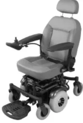
Milpet started as a Quickie S-11 motorized wheelchair shown in Figure 3.1. All of

the electronics besides the motors were removed so they could be replaced by new

components and circuitry. The goal of the redesign was to create a hardware/software

platform that could be used for many different aspects of autonomous navigation

or component needed to be added. This influenced many of the design decisions of

the hardware platform.

Figure 3.1: Stock Quickie S-11 wheelchair.

represents a subsystem of the hardware system, and the lines between them represent

how the systems interact. Most interactions stem from the power system as this is

the subsystem that takes in the 24V from the batteries and converts it to the voltages

required by the other subsystems. This system also provides many safety features for

both the other components and the users. Other subsystems include the embedded

Personal Computer (PC), which functions as the computation center for the entire

system, a microcontroller to handle the low-level hardware control, motors, and the

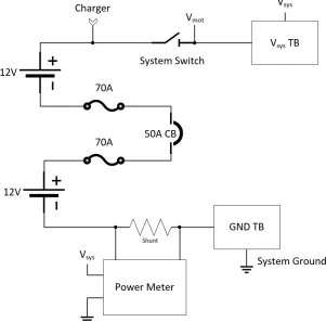
various sensors. Figure 3.3 shows the circuit diagram for the battery system.

Figure 3.3: Circuit diagram for the battery system of Milpet.

The battery system circuitry, shown in Figure 3.3, shows how the two 12V batteries

are wired together and some of the protection circuitry. The two batteries are wired

in series to achieve the necessary 24V system voltage. Each battery has an in-line

The batteries together have a 50-amp circuit breaker as over-current protection. The

system voltage is wired through a main switch to allow the entire system to switched

on and off. Also included is a power meter that continuously displays system voltage

and the current draw, measured via a low-value shunt resistor. Figure 3.3 also shows

where the battery charger is wired, where the motor driver is wired, and that terminal

blocks (TB) were used for system voltage and system ground. This system mainly

feeds the power system seen in Figure 3.4.

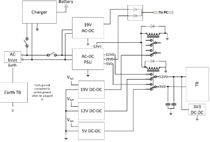
Figure 3.4: Circuit diagram for the power system of Milpet.

The power subsystem, seen in Figure 3.4, handles converting the 24V Direct

Cur-rent (DC) from the batteries to all of the voltages required by other components.

This system is also responsible for charging the batteries and allowing for the agent

to be powered entirely from a standard 120V Alternating Current (AC) source. The

entire system requires four different voltages: 19V, 12V, 5V, and 3.3V for various

120-V AC source, each of the required voltages, with the exception of 3.3V, can be

generated from battery power or a standard wall outlet. To generate these voltages

from the battery three separate DC to DC regulators are used for 19V, 12V, and 5V

(shown in Figure 3.4 as “DC-DC”). To generate the required voltages from the 120V

AC source two separate power supplies are used; one to generate 19V DC (labeled

“19V AC-DC”) and one to generate 12V and 5V DC (labeled “AC-DC PSU”).

Milpet also has the ability to switch between battery power and AC while running

without interruption. For the 12V and 5V rails this is handled by a Double Pull,

Double Throw (DPDT) relay. The coil of the relay is powered by a third rail

(-12V) of the “AC-DC PSU.” This was done so that when the AC-DC power supply

is powered on, the relay will switch the 12V and 5V rails of the system to the ones

generated by the AC-DC supply rather than the ones generated from the DC-DC

supplies. Large capacitors were also added to the two rails to facilitate switching

times. The 19V rail switching is handled slightly differently due to the fact that it

is generated by a separate supply. Both the AC and battery generated 19V rails are

wired through diodes into a single line that powers the PC. This means both supplies

are connected at all times so there is no need to physically switch between them. The

diodes are used to prevent current from one supply from flowing back into the other

supply if both supplies are active. This system works by allowing current to flow from

either supply depending on which is at a higher voltage. So, current will flow from

whichever supply is powered or, if both supplies are powered, current will flow from

the AC-DC supply as it outputs a slightly higher voltage. The 3.3V rail is generated

from the 12V rail so it does not require switching as the 12V rail is already properly

switched.

Figure 3.4 also shows how the AC input to the agent is handled and how the

charger is wired. On the wheelchair there is a standard C13 inlet for 120V AC that is

all grounds in the system are unified. From there, the neutral line is wired directly to

the charger and the two AC supplies while the hot line is wired through two Single

Pole, Single Throw (SPST) switches. These switches are wired to the charger and the

two AC supplies allowing for them to switched on and off. The output of the charger

is then wired back to the batteries (shown in Figure 3.3), and the AC supplies are

wired into the switching circuitry previously mentioned.

Figure 3.5: Circuit diagram for the motor and encoder system of Milpet.

Figure 3.5 shows the circuit diagram for the motor subsystem. The system

in-cludes the motors themselves, wheel encoders, and the motor driver. The motors are

the same motors that were equipped to the wheelchair from the factory. Not much

information is provided besides that they are standard brushed DC motors. Attached

to the motor shaft are a pair of rotary encoders, specifically Omron E6B2-CWZ1X

1000 P/R. A diagram of some of the internals of the encoder is shown in Appendix

A. These encoders are industrial quadrature encoders that have 1000 pulses per

revo-lution of the encoder shaft. Since the encoders are located on the motor shaft, rather

than the wheels themselves, the 20:1 gear ratio results in 20,000 pulses per wheel

revolution. The encoders allow for the agent to accurately measure the change in

distance for shorter distances. Over time however, small errors, caused by wheel

them as a valid option for long-term localization. The two output channels of each

encoder are wired to the microcontroller which keeps track of the count. Since the

encoders have an open-collector output, pull-up resistors are needed for each output

channel.

The motor driver is a Sabertooth 2x60 by Dimension Engineering. The Sabertooth

2x60 is a dual output motor driver capable of 60 amps continuous current on each

channel which is beyond adequate for the provided motors. This particular motor

driver can be controlled using analog voltages, servo commands, or serial commands.

For this application, serial commands are used and are generated by the

microcon-troller. Serial commands provide the most flexible solution and allow for the use of

the emergency stop functionality of the Sabertooth. The outputs of the motor driver

are wired directly to the motors. The large black bars in Figure 3.5 are ferrite cores

that prevent any high frequency noise from reaching the motors. The motor driver

and motors are powered directly from the batteries as shown in Figure 3.3. The

Sabertooth contains a separate input for emergency stop functionality which is wired

to the emergency stop system of the agent shown in Figure 3.6.

Figure 3.6: Circuit diagram for the emergency stop system of Milpet.

Figure 3.6 shows the emergency stop circuitry used on the agent. The Sabertooth

motor controller has built-in emergency stop functionality (when running in serial

mode) that provides an easy way to emergency stop the motors. The stop signal on