City, University of London Institutional Repository
Citation
: Apostolopoulou, D. & McCulloch, M. (2017). Cascade Hydroelectric Power
System Model and its Application to an Optimal Dispatch Design. Paper presented at the
IREP’2017 - 10th Bulk Power Systems Dynamics and Control Symposium, 27 Aug - 1 Sep
2017, Espinho, Portugal.
This is the accepted version of the paper.
This version of the publication may differ from the final published
version.
Permanent repository link:
http://openaccess.city.ac.uk/19442/
Link to published version
:
Copyright and reuse:
City Research Online aims to make research
outputs of City, University of London available to a wider audience.
Copyright and Moral Rights remain with the author(s) and/or copyright
holders. URLs from City Research Online may be freely distributed and
linked to.
City Research Online:
http://openaccess.city.ac.uk/
[email protected]
IREP’2017 - 10th Bulk Power Systems Dynamics and Control Symposium, Aug. 27-Sep. 1, 2017, Espinho, Portugal
Cascade Hydroelectric Power System Model and its
Application to an Optimal Dispatch Design
Dimitra Apostolopoulou and Malcolm McCulloch
Department of Engineering Science University of Oxford Oxford, UK OX1 3PJ
Email:{dimitra.apostolopoulou, malcolm.mcculloch}@eng.ox.ac.uk
Abstract—In this paper we propose an optimal dispatch scheme for a cascade hydroelectric power system that maximises the system efficiency, and minimises the spillage effects. Our approach proposes a methodology that has low computational burden and may be implemented for the short-term operation of a cascade hydroelectric power system. To this end, the non-linear relationships that describe the system physical constraints, e.g., power output, are transformed into affine relationships; thus reducing the computational complexity. The transformations are based on the construction of convex envelopes around bilinear functions; piecewise affine functions; and exploitation of optimisation properties. We demonstrate the efficacy of the proposed methodology with the Seven Forks system located in Kenya, and evaluate the performance of our method in terms of water volume and potential energy saved.
I. INTRODUCTION
The last years there has been an increase of renewable-based resource penetration into the electric grid that leads to the gradual de-carbonization of the energy supply sector [1]. Apart from a 40% reduction in greenhouse gas emissions and a 30% improvement in Energy Efficiency, the 2030 EU-wide targets set a minimum of at least 27% share of renewable energy resources in the energy consumption. However, renewable resources have unique characteristics and their integration raises several challenges into power systems operation. The variability of the renewable-based generation requires that the system has enough ramping capability to follow the net load variations in different time frames, ranging from seconds to hours. Furthermore, there is an increase in the need for balanc-ing services, larger reserves for the frequency control, as well as better ramping capability. There are several technologies available that may satisfy these needs. However, they are often associated with either additional cost or partial loss of the energy output. In this regard, appropriate use of existing resources, such as hydroelectric power systems, without any extra cost are worth to be investigated. Hydroelectric power systems are fitting candidates since they have good ramping capability and energy storage possibility in form of hydro reservoirs. Thus, they may be used to smooth the output of renewable-based generation and resolve any potential prob-lems caused to the grid due to solar output variability and intermittency.
In this regard, hydroelectric power systems may be used as “storage” devices for renewable generation. Cascade hydro-electric power systems are usually coupled both hydro-electrically,
i.e., they are used to meet same load; and hydraulically, i.e., the water outflow from one hydroelectric power plant is a significant portion of the inflow to the downstream plants [2, Ch. 7]. These relationships result in non-linear and non-convex expressions that are due to the spatial-temporal coupling among reservoirs; and for every plant, the nonlinear dependence between the power output, the water discharged, and the head of the associated reservoir. Such an event is a challenge for independent system operators (ISOs), who are responsible for the operation of hydroelectric power plants and. do not usually have optimisation tools to efficiently use the generation resources [3]. There is a need to develop cascade hydroelectric power system dispatch tools that provide a balance between accuracy and complexity; and may be used for the short-term operation of cascade hydroelectric power plants.
Several papers have addressed the problem of investigating the new role of hydroelectric power systems in the power systems paradigm. The authors in [4] show that hydroelectric systems play an important role in future power systems, where renewable resources are present, and support system adequacy in case of supply shortfall. In [5] the coordination of hydro-electric systems and wind generators in order to minimise wind energy curtailments during congestion situations is analysed. A case study on using a cascaded hydropower system to firm wind generation is presented in [6]. In [7] a global optimi-sation of the short term scheduling for hydroelectric power generation with mixed integer nonlinear programming formu-lation of a cascade of hydro plants is presented. However, in a security constrained short-term hydrothermal dispatch problem for large-scale systems simplified models are also necessary as discussed in [8]. The authors in [9] propose a semidefinite programming method to solve a hydrothermal coordination problem; they reformulate and relax the non-convex constraints associated with hydroelectric power system while guaranteeing global optimality.
maximum efficiency of the hydroelectric power plant occurs when the reservoir is full because the power output for a given amount of water is higher. In this regard, we construct the cas-cade hydroelectric system optimal dispatch by appropriately choosing the objective function, i.e., maximise the water level in the dam, and representing the physical and power balance constraints. Unfortunately, the constructed problem contains a linear objective function but non-convex (bilinear) constraints. This formulation needs to be relaxed in an efficient manner so that its actual implementation in the short-term operation of a cascade hydroelectric power system is realistic. To this end, the non-linear terms are relaxed by the construction of convex envelopes around the bilinear functions; piecewise affine functions; and exploitation of optimisation properties of the simplex method. We demonstrate the implementation of the proposed methodology in a real cascade hydroelectric power system the Seven Forks system in Kenya, which consists of five hydroelectric power plants.
II. PRELIMINARIES
In this section, we introduce the hydropower function and the scheduling constraints that are utilised to develop our framework. We consider a hydroelectric power system with
N hydroelectric power plants indexed by N = {1, . . . , N}
that we wish to schedule for a time periodT ={T1, . . . , TT},
which correspond to hourly intervals.
A hydroelectric power plant i∈ N may be characterised by its input-output curves. The input is in terms of water discharge and the output is in terms of power generation. The power generated by a hydroelectric power plant depends on the characteristics of the net hydraulic head, i.e., the difference between the level of the reservoir and the tail water, and the water discharge. In particular, the power of a hydroelectric power plant iat timet is defined as
PHit =ηi(hit, qit)ρ g hitqit,∀i∈N ,∀t∈T, (1)
where ρ is the density of the water in kg/m3; g is the gravitational acceleration in m/s2; hit is the net head of
water (the difference in water level between upstream and downstream of the turbine) of hydropower plant i at time t
in m;qit is the discharge of water of plantiduring timetin
m3/s;ηit(hit, qit)is the efficiency of the turbine generator at
head hit and dischargeqit.
The output of a hydroelectric power system is used to meet the load at every time instant t∈T. In this regard, we have
X
i∈N
PHit =PLt,∀t∈T, (2)
wherePLt is the load at timet. We should take into account
that the power output of each hydroelectric power planti∈N
is constrained by a minimum and a maximum output, i.e.,
PHmi ≤ PHit ≤ P
M
Hi, for all t ∈ T. Similar statements are
true for the head levels and the water discharge rates. Thus, we have that hm
i ≤ hit ≤ h
M
i and qmi ≤qit ≤ q
M i for all
t∈T andi∈N .
Another physical constraint that needs to be taken into consideration in the operation of a cascade hydroelectric power
1
2
N
r1t q1t
s1t
q2t
s2t
qNt
sNt
i
Hydroelectric Power Plant i
..
.
[image:3.612.323.550.60.138.2]r2t rN−1t
Fig. 1: Schematic representation of a hydroelectric power system.
system is the water balance between reservoirs. This balance equation relates the live volumes of the reservoirs, total discharges, spillages, and inflows. Evaporation and percolation losses may be included into the expected inflows; thus there is no need to be considered separately. Furthermore, in most cases there is a delay in the flow of water between reservoirs that needs to be accounted for in the modelling. A schematic representation of the cascade hydroelectric power system de-noted byN is depicted in Fig. 1. A mathematical formulation of the water balance of the cascade hydroelectric power system with the use of the hydraulic continuity equations is given below:
V1t = V1t−1+r1t−q1t−s1t, (3)
V2t = V2t−1+r2t+q1t−τ1 +s1t−τ1 −q2t−s2t, (4)
.. .
VNt = VNt−1+rN−1t+qN−1t−τN−1 +sN−1t−τN−1
−qNt−sNt, (5)
whereVit is the live volume of hydroelectric power plantiat
the end of timetin m3;τiis the time delay between reservoir
iandi+ 1, i.e., the time water needs to travel from one to the other;rit is the inflow into hydroelectric power plantiduring
time to t;sit is the spillage discharge of hydroelectric power
plantiduring time tot. There are constraints associated with the reservoir storage volume limits of each hydroelectric power planti∈N, which are defined as Vm
i ≤Vit ≤V
M i , for all
t∈T. Some additional physical constraints that may be taken into consideration are the initial and terminal reservoir storage volumes, i.e., Vi1 =Vistart andViT =Viend for alli∈N .
The modelling of water stored in a reservoir and its mapping to a certain head level is important since it relates (1) with (3)-(5). This relationship in most reservoirs is determined from topographical surveys of the dam site and is highly non convex [10]. We denote this relationship byhit =φi(Vit), for
alli∈N andt∈T.
III. HYDROELECTRICSYSTEMOPTIMALDISPATCH
it may be seen in (1). To this end, we wish to maximise the head of each reservoir at every time instant, i.e., hit, for all
i ∈ N, t ∈ T. The minimisation of the spillage effects are accomplished by including in the objective function the term
P
t∈T Pi∈N M sit. Then, the optimal dispatch is given by
maximise
hit,Pit,sit Vit,qit
subject to
X
t∈T
X
i∈N
hit−
X
t∈T
X
i∈N
M sit
X
i∈N
PHit =PLt,∀t∈T
PHit =ηi(hit, qit)ρ g hitqit,∀i∈N ,∀t∈T
V1t =V1t−1+r1t−q1t−s1t,∀t∈T \ {T1, TT}
Vit =Vit−1+ri−1t+qi−1t−τi−1+si−1t−τi−1 −qit−sit,∀i∈N \ {1},∀t∈T \ {T1, TT}
Vi1 =Vistart, ∀i∈N ViT =Viend, ∀i∈N
hit =φi(Vit), ∀i∈N , t∈T
Vim≤Vit ≤V
M
i , ∀i∈N , t∈T
qmi ≤qit ≤q
M
i , ∀i∈N , t∈T
hmi ≤hit ≤h
M
i , ∀i∈N , t∈T
PHmi ≤PHit ≤P
M
Hi, ∀i∈N , t∈T
(Vit−V
M
i )sit = 0, ∀i∈N , t∈T
sit ≥0, ∀i∈N , t∈T,
(6) whereτ=max{τ1, . . . , τN−1}is the maximum of the delays
andT1> τ; andM is a large positive number. The output of
(6) determines the head levels, power output, volume, spillage and water discharge for every hydroelectric power plant at every time instant in the period of interest. As it may be seen (6) has a linear objective function with linear and non-linear constraints. In order to solve (6) several algorithms may be used, e.g., the gradient method. However, this optimisation problem provides the output of a cascade hydroelectric power system in short time scales; thus, needs to be computationally efficient.To this end, we relax the original optimal dispatch problem given in (6).
A. Relaxations of Original Problem
The non-linear constraints of (6) refer to (i) the out-put of a hydroelectric power system, i.e., PHit =
ηi(hit, qit)ρ g hitqit,∀i ∈N ,∀t ∈T; (ii) the mapping of
the head level to the volume, i.e.,hit=φi(Vit), ∀i∈N , t∈
T; and the spillage effects, i.e., (Vit −V
M
i )sit = 0, ∀i ∈
N , t∈T. The objective is to transform these constraints and turn (6) into a linear optimisation problem, which has very low computational burden to solve with existing techniques.
The non-convex relationship of the output of a hydroelectric power system, the head and the water discharge is a bilinear function for a constant turbine efficiency. We assume the efficiency is constant, i.e.,ηi(hit, qit) =ηiand replace the
re-maining bilinear term with a convex envelope consisting of lin-ear over- and underestimating inequality constraints to
trans-form the non-convex constraint into a set of linear inequality constraints. In particular, we have thatPHit =aihitqit, with
ai =ηiρ g, andqmi ≤qit ≤q
M
i , hmi ≤hit ≤h
M
i . By using
McCormick’s envelopes (e.g., [11]), we obtain:
PHit ≥ qimhit+h
m i qit−h
m
i qim, (7)
PHit ≥ qiMhit+h
M i qit −h
M
i qiM, (8)
PHit ≤ qimhit+h
M i qit−h
M
i qim, (9)
PHit ≤ q
M i hit+h
m i qit−h
m
i qiM. (10)
One of the most useful applications of the piecewise linear representation is for approximating nonlinear functions. In this regard, we convert the non-linear mapping of the head level to the volume, i.e., hit =φi(Vit) to a piecewise affine
relationship. We consider k = 1, . . . , K intervals and thus have:
hit =β
k ivkit+γ
k
i, vkit ∈[ζk, ζk+1], fork= 1, . . . , K, (11)
where βk
i, γik ∈ R+ = {x ∈ R|x ≥ 0}, for k = 1, . . . , K,
ζ1 < ζ2· · · < ζK+1, vkit ∈ R
+ with V
it =
PK
k=1vkit. An
analysis of the piecewise affine approximation of the head to the volume of existing reservoirs based on data found in [12] showed that β1
i > βi2 > · · · > βiK. Usually,
piecewise linear functions are formulated as mixed integer programming problems, which would increase the complexity of (6). However, a special case for representing piecewise linear functions arises when diseconomies of scale apply, i.e., whenβ1
i > β2i >· · ·> βiKand we are maximisinghit, which
is this case (e.g. [13]). Thus, (11) may be rewritten as
hit =
K
X
k=1
(βikvkit)+γ
1
i, vkit ∈[0, ζk+1−ζk], for k= 1, . . . , K.
(12) Notice the slight abuse of notation with the term vk
it, which
represents different quantities in (11) and (12); the interpreta-tion will always be clear from the context.
The spillage effects, sit are included in the modelling
with (3)-(5). In the absence of spillage (3)-(5) would be satisfied withsit = 0. Thus, we may seesit as an “artificial”
variable that increases the feasible space of the problem and also has a physical meaning. The optimal dispatch objective function is designed to minimise the spillage effects, i.e., make
sit = 0 when it is feasible. The same concept is true for
nonbasic (and hence zero) is also a basic feasible solution to the original problem. The corresponding basis can be used as an initial basis for the original problem. Thus, we argue that by including sit in the objective function multiplied with a
large positive number M, then it will non zero only when
Vit−1 +ri−1t +qi−1t−τi−1 > V
M
i ⇒ Vit > V
M i . When
Vit < V
M
i , then sit = 0 as explained above. As a result,
the non-linear constraint (Vit−V
M
i )sit = 0 is satisfied and
does not need to be included in (6).
B. Overall Framework
The proposed optimal dispatch of a hydroelectric power system given in (6) may be rewritten in its relaxed form as
maximise
hit,Pit,sit Vit,qit,vk
it
subject to
X
t∈T
X
i∈N
hit−
X
t∈T
X
i∈N
M sit
X
i∈N
PHit =PLt,∀t∈T
V1t =V1t−1+r1t−q1t−s1t,∀t∈T \ {T1, TT}
Vit=Vit−1+ri−1t+qi−1t−τi−1 +si−1t−τi−1 −qit−sit,∀i∈N \ {1},∀t∈T \ {T1, TT}
Vi1=Vistart, ∀i∈N ViT =Viend, ∀i∈N
hit =
K
X
k=1 (βk
ivikt) +γ
1
i, ∀i∈N , t∈T
Vit=
K
X
k=1
vkit, ∀i∈N , t∈T
Vim≤Vit ≤V
M
i , ∀i∈N , t∈T
qim≤qit ≤q
M
i , ∀i∈N, t∈T
hmi ≤hit ≤h
M
i , ∀i∈N , t∈T
PHmi ≤PHit ≤P
M
Hi, ∀i∈N, t∈T
sit ≥0, ∀i∈N, t∈T,
0≤vikt ≤ζk+1−ζk, k= 1, . . . , K,∀i∈N , t∈T,
PHit ≥q
m i hit+h
m i qit−h
m
i qim,∀i∈N , t∈T,
PHit ≥qiMhit+h
M i qit−h
M
i qMi ,∀i∈N , t∈T,
PHit ≤q
m i hit+h
M i qit−h
M
i qim,∀i∈N , t∈T,
PHit ≤qiMhit+h
m i qit−h
m
i qiM,∀i∈N , t∈T.
(13)
Reservoir Masinga Kamburu Gitaru Kindaruma Kiambere
PM
i [MW] 40 93 225 72 165
VM
i [Mm3] 1753 133 21 10 519
hM
i [m] 51 78 140 35 151
hm
i [m] 25 61 131 31 134
qM
i [m3/s] 198.8 161.82 189 265.68 132
[image:5.612.333.539.598.708.2]ηi variable 0.9 0.92 0.89 0.9
TABLE I: Seven Forks system data.
IV. NUMERICALEXAMPLES
In this section, we illustrate the proposed optimal dispatch of a cascade hydroelectric power system with the Seven Forks system in Kenya, which consists of five hydroelectric power plants [10]. The time horizon we wish to schedule its operation is for a one year period with daily schedules. The constraints of the Seven Forks systems cascade in terms of power output, live volume, head, and turbine efficiency characteristics may be found in [12] and are shown in Table I. The minimum power output, live volume, and water discharge rate for all reservoirs are zero, i.e., Pm
i = 0, Vim = 0, qim = 0 for
i= 1, . . . ,5. In order to determinePLtfort∈T for the entire
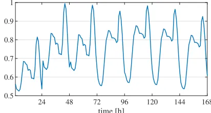
year we use a scaled version of the national load of Kenya for 2011, which was provided to us through Kenya Electricity Generating Company (KenGen). In order to make sure that the installed capacity of the hydroelectric power system is sufficient, we constrain the load to a maximum value of500
MW. A typical daily normalised demand profile for Kenya was used [15] is depicted in Fig. 2.
In order to construct the relaxed problem, as described in Section III-A, we approximate the relationship between the head levels and the live volume with a piecewise affine function. We use the data provided in [12] and in Fig. 3, we depict the actual relationship and the piecewise affine approximation between the head level and live volume for the Gitaru reservoir. As it may be seen the error introduced is marginal. For all the dams, we choose K = 3, i.e., we calculate the piecewise affine functions into three segments. For the five reservoirs we have:
h1t = 0.0281v
1
1t+ 0.0131v
2
1t+ 0.0084v
3 1t+ 25,
h2t = 0.3077v
1
2t+ 0.1351v
2
2t+ 0.0964v
3 2t+ 61,
h3t = 0.6349v
1
3t+ 0.4301v
2
3t+ 0.1667v
3 3t+ 131,
h4t = 0.5779v
1
4t+ 0.4117v
2
4t+ 0.2955v
3 4t+ 31,
h5t = 0.0648v
1
5t+ 0.0468v
2
5t+ 0.0398v
3 5t+ 134,
with v1
1t ∈ [0,400], v
2
1t ∈ [0,731], v
3
1t ∈ [0,622]; v
1 2t ∈
[0,14], v2
2t ∈ [0,37], v
3
2t ∈ [0,82]; v
1
3t ∈ [0,6], v
2 3t ∈
[0,9], v3
3t ∈ [0,6]; v
1
4t ∈ [0,4], v
2
4t ∈ [0,3], v
3
4t ∈ [0,3]; and
v1
5t ∈[0,292], v
2
5t ∈ [0,137], v
3
5t ∈[0,90]. The units for the
live volumes are in Mm3 and for the head in m.
KenGen also provided hourly historical data of the inflow data for all the hydroelectric power system from July 2015-June 2016. In the Seven Forks system there are three main
24 48 72 96 120 144 168
[image:5.612.51.305.633.704.2]time [h] 0.5 0.6 0.7 0.8 0.9 1
0 5 10 15 20 130
132 134 136 138 140
actual
[image:6.612.58.283.44.158.2]piecewise linear approximation
Fig. 3: Head level and live volume for Gitaru reservoir.
inflow streams; in Masinga, Kamburu and Kiambere. The remaining inflow into the dams is due to rainfall data. Based on these data, the time delay between all dams was deter-mined to be: Masigna-Kamburu, τ1 = 2 hours;
Kamburu-Gitaru, τ2 = 0 < 1 hour; Gitaru-Kindaruma, τ3 = 0 < 1
hour; and Kindaruma-Kiambere, τ4 = 4 hours. The starting
volume constraint for each reservoir is: V1start = 1173 Mm
3; V2start = 118 Mm
3; V
3start = 13 Mm
3; V
4start = 4 Mm
3; and V5start = 420Mm
3. There is no ending volume constraint.
In order to solve (13), we define M to be108. In order to
test the performance of the proposed dispatch we run compare the results between two methods: (i) dispatch proportional to the maximum capacity of each hydroelectric power plant; and (ii) proposed optimal cascade hydroelectric power plant dispatch. The average daily live volume is a lot higher for method (ii) compared to (i); thus the resiliency of the system is increased. In particular, the daily live volume for method (i) is 2,006 Mm3 and method (ii) 2,070 Mm3 and the daily potential energy was increased by 5%. Method (ii) tries to maximise the head levels; thus keeps the Gitaru head to high value increasing the dam’s efficiency. It should be noted that Gitaru is the largest in capacity dam, as depicted in Fig. 4.
V. CONCLUDINGREMARKS ANDEXTENSIONS
In this paper, we proposed an optimal dispatch scheme for the short-term operation of a cascade hydroelectric power system. More specifically, we constructed a non-linear opti-misation problem that represents explicitly the physical con-straints of hydroelectric power systems; and relaxed it to a linear optimisation problem that may be used for short-term operation of cascade hydroelectric power plants. In the
Jul '15 Oct '15 Jan '16 Apr '16 Jul '16
130 132 134 136 138 140
142 Method (i)
Method (ii)
Fig. 4: Head level of Gitaru dam with the two methods.
numerical studies, we showed that the proposed approximation provides a good representation of the actual state of the hydroelectric power system and the associated benefits with using the proposed framework in terms of the live volume of water used. The excess of water increases the resiliency of the electric system in dry seasons. In the future, we will demonstrate that the coupling of hydroelectric and solar technology is beneficial due to the negative correlation of rain and sunshine. In addition, we plan on incorporating uncertainty sources into the forecasts of the load that the hydroelectric power system is required to meet, i.e., uncertainty in load variations.
ACKNOWLEDGEMENT
The authors would like to thank Kenya Electricity Generat-ing Company for providGenerat-ing useful data for the case study and support in making this work possible.
REFERENCES
[1] J. Delbeke and P. Vis, “EU Climate Policy Explained,” European Union, Tech. Rep.
[2] A. J. Wood and B. F. Wollenberg,Power Generation, Operation, and Control, ser. A Wiley-Interscience publication. Wiley, 1996. [3] M. Cordova, E. Finardi, F. Ribas, V. de Matos, and M. Scuzziato,
“Performance evaluation and energy production optimization in the real-time operation of hydropower plants,”Electric Power Systems Research, vol. 116, pp. 201 – 207, 2014.
[4] A. V. Ntomaris and A. G. Bakirtzis, “Stochastic scheduling of hybrid power stations in insular power systems with high wind penetration,”
IEEE Transactions on Power Systems, vol. 31, no. 5, pp. 3424–3436, Sep. 2016.
[5] J. Matevosyan, M. Olsson, and L. S¨oder, “Hydropower planning coordi-nated with wind power in areas with congestion problems for trading on the spot and the regulating market,”Electric Power Systems Research, vol. 79, no. 1, pp. 39 – 48, 2009.
[6] A. Hamann and G. Hug, “Using cascaded hydropower like a battery to firm variable wind generation,” inIEEE Power and Energy Society General Meeting, Jul. 2016, pp. 1–5.
[7] R. M. Lima, M. G. Marcovecchio, A. Q. Novais, and I. E. Grossmann, “On the computational studies of deterministic global optimization of head dependent short-term hydro scheduling,” IEEE Transactions on Power Systems, vol. 28, no. 4, pp. 4336–4347, Nov. 2013.
[8] A. L. Diniz and M. E. P. Maceira, “A four-dimensional model of hydro generation for the short-term hydrothermal dispatch problem considering head and spillage effects,”IEEE Transactions on Power Systems, vol. 23, no. 3, pp. 1298–1308, Aug. 2008.
[9] Y. Zhu, J. Jian, J. Wu, and L. Yang, “Global optimization of non-convex hydro-thermal coordination based on semidefinite programming,”IEEE Transactions on Power Systems, vol. 28, no. 4, pp. 3720–3728, Nov. 2013.
[10] M. Mbuthia, “Hydroelectric system modelling for cascaded reservoir-type power stations in the lower tana river (seven forks scheme) in kenya,” in3rd AFRICON Conference, Sep. 1992, pp. 413–416. [11] F. A. Al-Khayyal and J. E. Falk, “Jointly constrained biconvex
program-ming,”Mathematics of Operations Research, vol. 8, no. 2, pp. 273–286, 1983.
[12] “Development of a power generation and transmission master plan, kenya,” Ministry of Energy and Petroleum, Republic of Kenya, Tech. Rep., May 2016.
[13] “Integer programming,” Massachusetts Institute of Technology, Tech. Rep.
[14] I. Griva, S. G. Nash, and A. Sofer,Linear and Nonlinear Optimization: Second Edition. Society for Industrial and Applied Mathematics (SIAM, 3600 Market Street, Floor 6, Philadelphia, PA 19104), 2009.
[image:6.612.55.290.576.697.2]