Qualitative Topological Coverage of Unknown Environments by Mobile Robots

(1)

University of Southampton Research Repository

ePrints Soton

Copyright © and Moral Rights for this thesis are retained by the author and/or other

copyright owners. A copy can be downloaded for personal non-commercial

research or study, without prior permission or charge. This thesis cannot be

reproduced or quoted extensively from without first obtaining permission in writing

from the copyright holder/s. The content must not be changed in any way or sold

commercially in any format or medium without the formal permission of the

copyright holders.

When referring to this work, full bibliographic details including the author, title,

awarding institution and date of the thesis must be given e.g.

AUTHOR (year of submission) "Full thesis title", University of Southampton, name

of the University School or Department, PhD Thesis, pagination

(2)

Department of Electrical and Computer Engineering The University of Auckland

New Zealand

Qualitative Topological

Coverage of Unknown

Environments by Mobile Robots

Sylvia Wong

February 2006

Supervisors: Dr Bruce A. MacDonald

Dr George Coghill

A        

(3)

(4)

Abstract

This thesis considers the problem of complete coverage of unknown environments by a mobile

robot. The goal of such navigation is for the robot to visit all reachable surfaces in an

envi-ronment. The task of achieving complete coverage in unknown environments can be broken

down into two smaller sub-tasks. The first is the construction of a spatial representation of the

environment with information gathered by the robot’s sensors. The second is the use of the

constructed model to plan complete coverage paths.

A topological map is used for planning coverage paths in this thesis. The landmarks in the

map are large scale features that occur naturally in the environment. Due to the qualitative

nature of topological maps, it is rather difficult to store information about what area the robot

has covered. This difficulty in storing coverage information is overcome by embedding a cell

decomposition, called slice decomposition, within the map. This is achieved using landmarks in the topological map as cell boundaries in slice decomposition. Slice decomposition is a new cell

decomposition method which uses the landmarks in the topological map as its cell boundaries. It

decomposes a given environment into non-overlapping cells, where each cell can be covered by

a robot following a zigzag pattern. A new coverage path planning algorithm, called topological

coverage algorithm, is developed to generate paths from the incomplete topological map/slice decomposition, thus allowing simultaneous exploration and coverage of the environment.

The need for different cell decompositions for coverage navigation was first recognised by

Choset. Trapezoidal decomposition, commonly used in point-to-point path planning, creates

cells that are unnecessarily small and inefficient for coverage. This is because trapezoidal

de-composition aims to create only convex cells. Thus, Choset proposed boustrophedon

decompo-sition. It introduced ideas on how to create larger cells that can be covered by a zigzag, which may not necessarily be convex. However, this work is conceptual and lacking in

implementa-tion details, especially for online creaimplementa-tion in unknown environments. It was later followed by

Morse decomposition, which addressed issues on implementation such as planning with

par-tial representation and cell boundary detection with range sensors. The work in this thesis was

developed concurrently with Morse decomposition.

(5)

ii ABSTRACT

Similar to Morse decomposition, slice decomposition also uses the concepts introduced by

boustrophedon decomposition. The main difference between Morse decomposition and slice

decomposition is in the choice of cell boundaries. Morse decomposition uses surface gradients.

As obstacles parallel to the sweep line are non-differentiable, rectilinear environments cannot

be handled by Morse decomposition. Also, wall following on all side boundaries of a cell is needed to discover connected adjacent cells. Therefore, a rectangular coverage pattern is used

instead of a zigzag. In comparison, slice decomposition uses topology changes and range sensor

thresholding as cell boundaries. Due to the use of simpler landmarks, slice decomposition can

handle a larger variety of environments, including ones with polygonal, elliptical and

rectilin-ear obstacles. Also, cell boundaries can be detected from all sides of a robot, allowing a zigzag

pattern to be used. As a result, the coverage path generated is shorter. This is because a zigzag

does not have any retracing, unlike the rectangular pattern.

The topological coverage algorithm was implemented and tested in both simulation and with a real robot. Simulation tests proved the correctness of the algorithm; while real robot tests

demonstrated its feasibility under inexact conditions with noisy sensors and actuators.

To evaluate experimental results quantitatively, two performance metrics were developed. While

there are metrics that measure the performance of coverage experiments in simulation, there are

no satisfactory ones for real robot tests. This thesis introduced techniques to measure eff

ective-ness and efficiency of real robot coverage experiments using computer vision techniques. The

two metrics were then applied to results from both simulated and real robot experiments. In simulation tests, 100% coverage was achieved for all experiments, with an average path length

of 1.08. In real robot tests, the average coverage and path length attained were 91.2% and 1.22

(6)

Acknowledgements

It has been a long time since I first arrived at the E&E department in the University of Auckland as a wide-eyed undergraduate. I am happy to have this opportunity to thank some of the people

who have helped make it an enjoyable experience.

First of all, I would like to thank my supervisor, Dr Bruce MacDonald for his support and

guidance throughout my PhD years. Without his encouragement and occasional stern looks, I

would not have been able to make it to the end.

I would also like to thank my parents. They provided much financial support, which is very

appreciated. I hope they feel proud when they see this 200 page masterpiece.

The technical staffin the department have also been of tremendous help. Lance Allen and the

workshop designed and built the wooden enclosure for the Khepera robot. Jamie Walker and

Evans Leung helped me with all sorts of computer and networking problems. Bev Painter,

Nichola Kavacevich and Grant Sargent have also been very helpful.

I greatly enjoyed the interactions with other PhD students in the department, from inspiring

technical discussions to playing age of empires. They are (in alphabetical order): GeoffBiggs,

Toby Collett, Barry Hsieh, Lee Middleton, Adrian Pais, Russell Smith, Brad Sowden, Chris

Waters, Joseph Wong and David Yuen.

Lastly, I would like to thank Jorge Cham, the creator of piled higher and deeper. His comic

strips provided me with laughter when I sorely needed it.

(7)

(8)

1

Introduction

1.1 Overview of problem domain

A

recent survey released by the UN Economic Commission for Europe [1, 41] reported

that robot orders for the first half of 2003 were the highest ever recorded. The survey

also predicts the worldwide growth rate of the robotic industry will average at 7.4%

annually for the period 2003 to 2006. Also, by the end of 2006, a tenfold increase in domestic

service robots is predicted. These statistics and predictions show that robots have moved out

of science fiction and into everyday life. Nowadays, it is already common to find industrial

robots working in hazardous environments or space rovers surveying Mars. In the foreseeable

future, domestic and service robots may also become a common sight. Examples include do-mestic robots mowing lawns and vacuuming floors autonomously, or professional service robots

assisting in surgeries and surveillance.

To be useful, a robot has to be skilled in the specific task it is designed for. For example, a lawnmowing robot needs to know how to operate the grass cutting tool it carries; or a rubbish

collecting robot needs to know how to pick up soft drink cans and cigarette butts. However,

these robots should also be equipped with more general abilities such as obstacle avoidance,

map building, path planning and localisation. These abilities enable a robot to move around its

environment to do its job efficiently and with minimum human intervention.

(13)

2 Introduction

One such general ability that is very important to all autonomous robots is path planning. Path

planning in robotics is the intelligence of finding a path in a map that leads from a start

config-uration to a goal configconfig-uration. This area of artificial intelligence has received a great deal of

attention in the robotics research literature [66, 76, 85, 91]. Path planning is an essential

com-ponent of robot manipulator controllers, as it is the the basis for describing and controlling the manipulator tip [42, 54]. It is also important for mobile robots, as it is the basis for describing

and controlling the varying robot positions in space [46, 98].

Most path planning algorithms are for point-to-point path planning. This type of algorithm

usually attempts to find the shortest or quickest path to get from one point to another. Though sometimes criteria other than path lengths are used [71]. However, in some applications, a

coverage path is needed instead. The aim of a coverage path planner is to create a path that

covers all surfaces in an environment. In other words, given an initial location, it does not

matter where the final location is, as long as the journey visits all surfaces in the environment.

Examples of robotic tasks that require a coverage path are cleaning [38], surface coating [86,

87], humanitarian demining [69] and foraging.

Coverage path planning is similar to exploration, but not the same. When exploring, a robot

sweeps its long range sensors, moving so as to sense all of its environment, often to build a

map. In a coverage application, the robot or a tool it carries must pass over all the floor surface.

Compared to point-to-point path planning, the coverage path planning problem has not received

as much attention. However, as robots move into service roles and interact with humans in

more varied environments for a wider range of tasks, coverage will become more important.

The ability to fully cover an environment will be a key capability for all mobile systems. For

example, domestic robot assistants can spend their idle time cleaning, collecting items and

storing them away.

Apart from generating different types of output, path planners also differ in their formats of

input (the map). As path planning is essentially a search on a map of the environment, the data

structure used to store this map naturally influences the operations of path planning algorithms.

Also, depending on the application domain, the environment the robot operates in maybe known

or unknown beforehand. If a map is created by a human operator and fed to the path planner,

the environment is known to the robot. If no map is provided, the environment is unknown,

and the robot has to construct a map for path planning using sensor information. There are two distinct ways to handle this situation. The first method is to carry out an exploration phase to

construct an accurate map [95, 107] before any path planning is done. The alternative is to make

assumptions concerning the unknown areas in the map in order to commence path planning, and

then update the planned path whenever new environmental information becomes available [58].

(14)

1.2 Applications of coverage path planning 3

1.2 Applications of coverage path planning

Coverage path planning is needed in a variety of mobile robot applications. The focus of this

thesis is on the coverage of flat, indoor, unknown surfaces populated with obstacles. It is also

assumed that the robot has to stay within the region. Typical applications that fit these criteria are vacuum cleaning and floor scrubbing.

Lawn mowing is very similar, but the restriction on staying within bounds is relaxed. For

example, it is perfectly acceptable to push the lawn mower over the footpath while cutting grass

on the kerb. Compared to a typical home or office, the average lawn is relatively free from

obstacles. Also, being an outdoor application, global positioning systems can be used to aid

localisation and landmark matching.

Intuitively, humanitarian demining should also allow the robot to stray outside the area to be

covered. However, since it is unknown whether the region outside is free of landmines, it is safer

and smarter to restrict movement within bounds of the environment. Also, due to the dangers of

the mines, the robot should not move into surfaces not scanned by the landmine detection tool

yet. Therefore, localisation must be very accurate. Otherwise, due to dead reckoning1_{error, the}

robot might move into an area it believes to be covered, but is not in reality.

In window cleaning the target surface is vertical, instead of horizontal. Other than this minor

difference, the coverage requirement is essentially the same as vacuum cleaning.

In machine milling, it might be desirable to mill only in one direction (either in the spindle

direction, or against). This means the coverage path should be a sequence of, say,

right-to-left movements, instead of alternate right-to-left-to-right and right-to-right-to-left movements. This is because

milling in only one direction gives better surface quality [51].

1.3 Description of the thesis

1.3.1 Scope of the research

The purpose of this research is to develop robust coverage algorithms for mobile robots working

in unknown environments. I do not assume known environments because it can be costly and

inflexible to require a complete map of the environment the robot operates in. In certain types

of robots, for example, domestic vacuum cleaners, owners generally lack the expertise to enter

detailed maps to the robots and will therefore require professional help for such tasks. Also, the map will need to be updated whenever the owner re-arranges the furniture.

(15)

4 Introduction

Map building is a key issue in this thesis because of the requirement of unknown environments.

The robot should simultaneously construct a map with sensor information while covering the

environment at the same time. This means that the coverage path planner has to make its

decision based on a partial map of the robot’s environment. Using a separate exploration phase

for map building purposes is considered inefficient because a coverage path already requires the

robot to visit all surfaces.

An integral part of developing a robotic coverage algorithm is to measure how well the

algo-rithm performs in experiments. Performance metrics allow quantitative evaluation of

implemen-tations. They also permit comparisons between different algorithms. Despite the importance of

quantitative metrics, this is an area that has received very minimal attention. Development of suitable performance metrics is therefore another aim of this research.

1.3.2 Overview of the thesis

The thesis is divided into the following chapters:

Chapter 2 presents a literature review of algorithms for coverage using mobile robots. The

review includes algorithms for both known and unknown environments. The chapter also

dis-cusses existing performance metrics for evaluating coverage algorithms in both simulation and

real robot experiments.

Chapter 3 presents the events and algorithms for slice decomposition. Two versions of the

decomposition are presented. The first one is for known environments, and is produced using

a normal line sweep process. The second one is for unknown environments, where the sweep

line will be limited to within free space.

Chapter 4 introduces the topological coverage algorithm. The algorithm creates a slice

decom-position of any environment online, without a known map. It explains methods for detecting

landmarks used to form the decomposition. It also talks about how slice decomposition is stored

in a topological map, how the map is maintained and updated, and how to determine if the map

is completed and the environment is completely covered. It also explains why travelling

be-tween regions is robust. Completeness and complexity of the decomposition are also discussed.

Chapter 5 introduces two new performance metrics for coverage experiments. The chapter also

includes practical methods for evaluating and measuring parameters needed to calculate these

metrics.

Chapter 6 focuses on the implementation of the topological coverage algorithm. It describes the

simulation and real robot environment and platform. It also talks about the implementation of

(16)

1.4 Contributions of the thesis 5

Chapter 7 shows results from experiments in simulation and with a real robot. The metrics

introduced in Chapter 5 are used to evaluate the performance of the experiments. The results

are also discussed and compared with existing coverage algorithms.

Chapter 8 presents a list of potential future work and some conclusions drawn from the research

in this thesis.

Appendix A describes an alternative method for recognising and classifying the landmarks used

in the topological map. Two types of neural networks are trained to learn the different

land-marks. This appendix gives a brief introduction to the two neural networks, followed by results

from landmark recognition tests.

Appendix B covers the computer vision techniques used in Chapter 5 for creating composite images in greater detail. Topics discussed include Canny edge detection and Hough transforms.

1.4 Contributions of the thesis

This thesis makes several significant contributions. A study in the existing literature provides

the basis for the identification of areas where contributions can be made to the field.

First is the development of an online coverage algorithm that uses a partial qualitative

topolog-ical map for planning. Previously, qualitative maps based on simple landmarks have only been

used in point-to-point path planning. This is because nodes and edges of topological maps do not correspond to specific locations in space. This qualitative nature makes it difficult to store

coverage information. The problem is overcome by using the landmarks as cell boundaries of

slice decomposition. In other words, the topological map embeds a slice decomposition of the

environment. As a result, even though individual nodes in the map are not associated with

spe-cific areas of space, a combination of nodes now defines a cell of the decomposition. Coverage

information is then stored with cells in slice decomposition.

Second is the introduction of slice decomposition, a cell decomposition for covering unknown

environments. It can handle a larger variety of environments than existing cell decomposition

based coverage algorithms. The concept of using the split and merge of the sweep line by

obstacles as cell boundaries was first introduced in boustrophedon decomposition [30]. This

approach creates maximum sized cells that can still be covered by a simple zigzag pattern. However, boustrophedon decomposition lacks detailed algorithms or implementation details.

Slice decomposition extends the split and merge concepts in boustrophedon decomposition.

New cell boundary types are added to simplify boundary detection in online decomposition

with range sensors. Similar to slice decomposition, Morse decomposition [8] is also for

(17)

6 Introduction

decomposition and slice decomposition is in the choice cell boundaries. Morse decomposition

uses surface gradients. As obstacles parallel to the sweep line are non-differentiable, rectilinear

environments cannot be handled by Morse decomposition. In comparison, slice decomposition

uses topology changes and range sensor thresholding as cell boundaries. Due to the use of

sim-pler landmarks, it can handle environments with polygonal, elliptical and rectilinear obstacles.

Thirdly, due to the use of simple landmarks as cell boundaries, the topological coverage

algo-rithm employs a shorter navigation pattern to cover each cell in the decomposition than Morse

decomposition. Wall following on side boundaries of cells is needed in Morse decomposition

to discover connected adjacent cells. This is because cell boundaries can only be detected when

they are the closest point on the obstacle surface from the robot compared to all other points

on the obstacle surface. Therefore, a rectangular pattern that includes retracing is used to cover

each cell in the decomposition. On the other hand, due to the use simpler landmarks and a more

general technique for landmark detection, the topological coverage algorithm allows a robot to detect events in slice decomposition from all sides. As a result, a simple zigzag path that

does not include any retracing can be employed instead. Due to the use of a shorter navigation

pattern to cover individual cells, the topological coverage algorithm generates coverage paths

that are shorter and more efficient.

Lastly, new performance metrics for evaluating real robot coverage experiments are developed.

Currently, results from real robot experiments are mostly presented qualitatively, showing

pic-tures of the routes taken by the robots. The only metric available is the coverage factor [22].

However, it does not measure effectiveness or efficiency of experiments properly. The two

met-rics proposed in this thesis measure the effectiveness and efficiency of any coverage experiment

using data collected with computer vision techniques. The methods used to collect the data are

(18)

Only in our dreams are we free. The rest of the time we need wages.

Terry Pratchett, “Wyrd Sisters”

2

Coverage navigation and path planning

P

ath planning for mobile robots generally involves a search on a spatial representation

(map) of the environment. Therefore mapping and path planning are two related issues

and cannot be examined in complete isolation. Robotic maps are data structures that

store information about the environment. For any given data structure, there are multiple ways

to conduct a search. For example, there are numerous search algorithms for graphs, such as A*

search and depth-first search [92]. In summary, there are many types of robotic maps, and even

more path planning algorithms.

This chapter first introduces several common robotic maps. They are Voronoi diagram

(Sec-tion 2.1), cell decomposi(Sec-tion (Sec(Sec-tion 2.2) and grid map (Sec(Sec-tion 2.3). These maps all employ

some form of space decomposition, where a complex space is repeatedly divided until simple

subregions of a particular type are created. Grid based maps are a special case of space

de-composition where the environment, both free space and obstacles, is decomposed into uniform

grid cells. Emphasis has been placed on space decomposition based maps as they are the most common data structure used in coverage path planning. This is because coverage algorithms

usually use the strategy of “divide and conquer”. Basically the environment is segmented into

simpler subregions, and each subregion is then covered in turn. Cell decomposition is favoured

by Choset, the leader in the area of robot coverage algorithms [8, 9, 11]; while grid maps are the

most common choice among researchers in mobile robot coverage [44, 97, 109].

(19)

8 Coverage navigation and path planning

Two other robotic mapping and path planning methods are also discussed. Even though they are

not based on space decomposition, they are included here because of their importance in mobile

robot navigation. The two methods are topological mapping (Section 2.4) and reactive robotics

(Section 2.5). Topological maps do not form precise geometric representations of space. Instead

the map describes spatial relationship in a qualitative way, much like the way humans describe their environments. Reactive robotics approaches the navigation problem from a non symbolic

AI perspective. As such, no maps are used and there is no planning of paths in the traditional

sense.

Section 2.8 contains a survey on the performance metrics used in simulated and real robot experiments of coverage algorithms. In also includes a brief discussion of the complexity, or

upper bound, of the length of a coverage path.

Lastly, this chapter finishes with a discussion that identifies areas where contributions can be

made.

2.1 Voronoi diagram

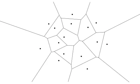
Perhaps the most popular space decomposition is the Voronoi diagram. It is used in a wide

range of disciplines including biology, computational geometry, crystallography and

meteorol-ogy [81].

Given a finite set of distinct points (called reference vectors) in the Euclidean plane, an ordinary Voronoi diagram is formed by associating all locations in that space with the closest member

of the point set with respect to the Euclidean distance. Thus a Voronoi diagram partitions the

space into a set of non-overlapping regions. Figure 2.1 shows a set of reference vectors with its

Voronoi diagram.

More formally, let the set of n reference points be P = {p1, . . . ,pn} ⊂ R2, and their Cartesian coordinates be x1, . . . ,xn. Then the ordinary Voronoi region associated with reference point pi

is given by

V(pi)= {x| kx−xik ≤ kx−xjkfor i , j}

And the set given by

V={V(p1), . . . ,V(pn)}

is the ordinary Voronoi diagram of the reference point set P.

By applying a distance measure other than Euclidean distance, the ordinary Voronoi diagram

has been extended or generalised in many directions [81]. One of the most useful generalisations

(20)

[image:20.595.88.535.83.352.2]

2.1 Voronoi diagram 9

Figure 2.1: Voronoi diagram for a set of reference points.

of a set of n obstacles A={A1, . . . ,An}, rather than a set of points. The area Voronoi diagram is

calculated using the following equation for the shortest distance from point p to obstacle Ai:

ds(p,Ai)=min xi

{kx−xik |xi ∈Ai}

In other words, an area Voronoi diagram (or simply generalised Voronoi diagram) is formed by

associating all locations in the free space of the robot’s environment with the closest obstacle.

Figure 2.2 shows an example of a generalised Voronoi diagram for an environment with two obstacles.

In robotics, generalised Voronoi diagrams have been used in path planning [66], topological

mapping [84] and localisation with visual landmarks [106]. A feature of maps based on

gener-alised Voronoi diagrams is that they maximise clearance between robot and obstacles. A robot following the map will be staying far from obstacles. As a result, the Voronoi diagram is

unde-sirable for coverage tasks. On the other hand, this characteristic makes it perfect for exploration

navigation with long range sensors. For example, Acar, Choset and Atkar used a map based on

the generalised Voronoi diagram for a robot equipped with an extended range landmine detector

(21)

[image:21.595.186.382.85.288.2]

Figure 2.2: The Voronoi diagram maximises clearance between robot and obstacles. (Reproduced from page 172 of [66]).

2.2 Cell decomposition

A cell decomposition divides a complex structure S into a collection of disjoint simpler

com-ponent cells. In exact cell decomposition, the union of the comcom-ponent cells is exactly S . While

in approximate cell decomposition, the union of the component cells is approximately S . The

boundary of a cell corresponds to a criticality1of some sort. The most common example of cell

decomposition is trapezoidal decomposition [66]. It is formed by sweeping a line across the environment, and maintaining a list D of cells that intersects with the sweep line. The history

of list D, ie all the cells that have appeared in D, forms the decomposition. A cell boundary is

created whenever a vertex is encountered. Due to the use of vertices as criticality, obstacles are

limited to polygons. Also, each cell of a trapezoidal decomposition is either a trapezoid or a

triangle. The algorithm for trapezoidal decomposition is shown in Algorithm 2.1.

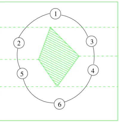
Figure 2.3 shows an example of trapezoidal decomposition for an environment with one

polyg-onal obstacle. Originally, the list D consists of only one cell, and thus D = (c1). At the first

vertex, cell c1 is split into two parts, and D changes to (c2,c3). For the next two vertices in the environment, cells are replaced only. The list D changes to (c2,c4) and then again to (c5,c4). Lastly, cells c4and c5are merged into one cell, and D becomes (c6).

The trapezoidal decomposition was originally proposed by Chazelle to partition a 3D

poly-hedron into a collection of convex polyhedra [29]. Other usages outside of robotics include

decomposing complex polygons in 2D computer graphics [88].

For path planning, the trapezoidal decomposition is first reduced to a connectivity graph that

1_{Criticalities in cell decompositions are conditions of the sweep line where, if satisfied, a new cell boundary is}

(22)

2.2 Cell decomposition 11 c1

c2 c3

c4

c5

c1

c2 c3

c4

c5

c6

sweep

direction

c1 c1

c2 c3

c4

D=(c2,c3) D=(c2,c4)

D=(c5,c4)

D=(c6)

(23)

12 Coverage navigation and path planning Algorithm 2.1 Trapezoidal Decomposition

yL: position of sweep line

{y1, . . . ,yn}: sorted list of y coordinates of all vertices in environment

D= (. . . ,ci−2,ci−1,ci,ci+1,ci+2, . . .)

for yL =y1to yndo

if vertex splits cell ciinto two then

(ci)←(cd,cd+1)

D= (. . . ,ci−2,ci−1,cd,cd+1,ci+1,ci+2, . . .)

else if vertex merges two cells ci and ci+1then (ci,ci+1)←(ce)

D= (. . . ,ci−2,ci−1,ce,ci+2, . . .)

else if vertex replaces cell ci with a new cell then

(ci)←(cf)

D= (. . . ,ci−2,ci−1,cf,ci+1,ci+2, . . .)

end if end for

represents the adjacency relation among the cells [66]. Then this associated connectivity graph is searched to find paths between any two cells. Figure 2.4 shows the connectivity graph for the

trapezoidal decomposition formed in Figure 2.3.

Choset first recognised that trapezoidal decomposition creates cells that are unnecessarily small,

and therefore inefficient, for coverage purposes [30, 32]. Trapezoidal decomposition creates

cells that are convex polygons only. However, non-convex cells can also be covered completely

by simple coverage patterns. A decomposition that creates more cells are less efficient because

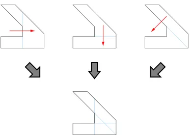
for each cell, additional motion along the cell boundary maybe required. For example, the two

cells on each side of the obstacle in Figure 2.5(a) can be merged and a simple zigzag pattern

can still cover the combined cells (Figure 2.5(b)).

Based on this concept of merging multiple cells in trapezoidal decomposition, Choset proposed the first exact cell decomposition specifically designed for coverage navigation [30]. The

result-ing decomposition is called boustrophedon2_{decomposition, signifying the relationship between}

the decomposition and the zigzag. Boustrophedon decomposition introduces the idea of using

the split and merge of the sweep line by obstacles as criticality. This is explained in the example

in Figure 2.6. However, [30] does not provide a detailed algorithm for the decomposition, nor

does it define the criticality precisely. Moreover, it is unclear if, or how, concave obstacles are

handled.

Huang attempted to reduce the cost of coverage by minimising the number of turns in the

coverage path [55]. He introduced the Minimal Sum of Altitude (MSA) decomposition. The

decomposition works on known polygonal environments. The basic premise behind MSA

de-2_{Alternately from right to left and from left to right, like the course of the plough in successive furrows (Oxford}

(24)

2.2 Cell decomposition 13

1

3 2

5 4

[image:24.595.213.413.119.323.2]

6

Figure 2.4: To form the associated connectivity graph, each cell is labelled by a distinct integer and connected to its neighbouring cells.

(a)

(b)

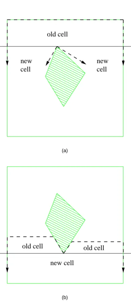
[image:24.595.101.528.433.676.2]

(25)

new cell old cell

new cell

(a)

new cell

old cell _{old cell}

[image:25.595.177.390.163.657.2]

(b)

(26)

(a) (b)

Figure 2.7: Assigning different sweep directions to cells can produce coverage paths with fewer turns. (Reproduced from [55]).

composition is that cost of coverage is lower when there are fewer turns in the path. This is

because a robot must slow down to make a turn. Huang assumed that the cost of travelling

between cells in the decomposition is significantly lower than the cost of turning. By choosing

different sweep directions for different cells, the cost of a coverage path can be lowered. This is

illustrated in the example in Figure 2.7.

The MSA decomposition is created with a two step process – multiple line sweeps followed by dynamic programming. For each edge orientation (of both the boundary of the environment

and all obstacles), a line sweep is performed. A cell boundary is created for each vertex at split

and merge events.3 _{The decompositions from all edge orientations are then overlaid upon each}

other. Figure 2.8 shows an example of this multiple line sweep decomposition process.

Once the initial decomposition from multiple line sweeps is formed, an adjacency graph is

created to represent the decomposition. An example of this graph is shown in Figure 2.9.

The basis of the dynamic programming step is to either split this graph in two, thus creating

two smaller subproblems; or to try to unite all cells and cover them as one large region. The minimum sum of altitudes of graph G is defined as:

S (G)=min

C(G),min

i S (G

i

1)+S (G

i

2)

(2.1)

where i iterates over all possible ways to split the graph G into two connected subgraphs G1

and G2. C(G) is the cost of covering all cells as one subregion. Figure 2.9 shows an example of

the first level of decomposing a problem. Figure 2.10 shows the final MSA decomposition for a simple environment.

3_{An event in a cell decomposition occurs when the sweep line encounters a criticality. Therefore, a duality}

(27)

[image:27.595.97.473.120.385.2]

Figure 2.8: The first step in creating a MSA decomposition is multiple line sweep. A line sweep is performed for each edge orientation. The decomposition of all the line sweeps are then overlaid on top of each other. (Reproduced from [55]).

(28)

(a)

(b)

Figure 2.10: MSA decomposition of a simple environment. (a) Initial decomposition from multiple line sweeps. (b) After dynamic programming. (Reproduced from [55]).

However, MSA decomposition is limited in the complexity of environments it can handle. This

is because of an exponential complexity for the algorithm. Firstly, each sweep direction

con-tributes a dividing line that divides many cells. This produces a large number of cells in the adjacency graph. Secondly, the dynamic programming phase must examine all connected

sub-graphs of 1 to n nodes for a graph of n nodes.

Both boustrophedon and MSA decompositions are defined only for known environments. The idea of using split and merge events of the sweep line as criticality was extended to unknown

environments in the works of Butler [22, 23] and Acar [8, 12]4_.

For a cell decomposition to be used for covering unknown environments, the following issues need to be addressed. Firstly, mobile robots can only move within the free space region of

the environment. As a result, the sweep direction can no longer be from top to bottom only.

For example, the area underneath the U-shaped obstacle in Figure 2.11 can only be swept in

the reverse (bottom to top) direction. Secondly, planning of the coverage path has to be done

using a partial cell decomposition of the environment. This is because the cell decomposition

has to be created simultaneously with the coverage process. Thirdly, criticalities can occur

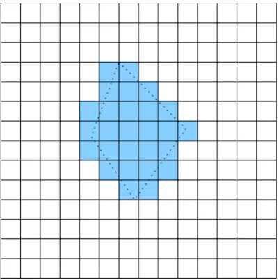
between sweep line positions. An example of which is shown in Figure 2.12, where the vertex

is positioned between strips of the zigzag. Lastly, the criticality chosen has to be realistically

detectable by robot sensors.

Butler et. al. proposed CCR, an exact cell decomposition for contact sensing robots5

cover-ing unknown rectilinear environments [23]. Cell boundaries are formed whenever an obstacle

boundary parallel to the sweep line is encountered. An example of CCRis shown in Figure 2.13.

4_{Butler and Acar were PhD students at the Robotics Institute at Carnegie Mellon University. Choset is a}

professor at the same institute, and is the supervisor of Acar.

(29)

[image:29.595.154.414.492.728.2]

18 Coverage navigation and path planning (a) (b)

Figure 2.11: Mobile robots cannot move inside obstacle space. (a) Sweep line is limited to the current free space cell. (b) Some cells must be swept in the reverse direction.

Figure 2.12: The vertex falls between two consecutive strips of a zigzag.

Figure 2.13:CCR uses an exact cell decomposition for rectilinear environments. (Reproduced from

(30)

intervals

Ciw Cj

∞

Cix

tr tl

bl

br

Figure 2.14: The partial decomposition inCCRis stored as a list of cellsC={C0, . . . ,Cn}. This diagram

shows the data structure associated with an individual cellCi, which is a member ofC, ie

Ci ∈C. CellCjis a neighbour ofCiand is shown here for clarity. (Adapted from page 17

of [22]).

The partial decomposition constructed is stored as a list of cells C= {C0, . . . ,Cn}. Figure 2.14

shows the data structures associated with each cell in CCR. Cix is the maximum possible extent

of cell Ci, and is represented simply by a rectangle. Cin is the cell’s minimum known extent, and

is given by four points – two on the cell’s right boundary (tr and br), and two on the cell’s left boundary (tl and bl). When the robot begins coverage with no knowledge of the environment,

C will contain a single cell C0 in which the minimum known extent C0n has zero size and

the maximum possible extent C0x is infinite in all directions. As the robot covers this cell, its

minimum known extent C0n will increase in size, while its maximum possible extent C0x will

be limited with the discovery of each boundary. In addition to the minimum and maximum

extents of the cell, the width of the portion of the cell that has been covered by the robot is

also represented (Ciw). Associated with each of the edges of the cell is a linked list of intervals

which explicitly denote the cell’s neighbours at each point along the edge. Each interval is

represented as a line segment together with a neighbour ID. A cell is complete when its edges are at known locations, it has been covered from side to side, and all sides have been completely

explored. In addition to the cell decomposition C, CCR maintains a list H = {H0, . . . ,Hm} of

placeholders. A placeholder is an element of the boundary of any cell in C that is not a boundary

of the environment, and thus are entrances to to free space cells. Coverage of an environment is

complete when no placeholders remain.

Normally, the robot follows the U-shaped pattern in Figure 2.15 to cover individual cells.

Seg-mentsαandδare sliding movements against the side boundaries of the cell. An event

(critical-ity) occurs whenever the robot is prevented from successfully executing the U-shaped coverage

pattern. Also, all the events defined in CCR can be detected without the use of any range

(31)

20 Coverage navigation and path planning β γ δ α

Figure 2.15: U-shaped coverage pattern used inCCR and Morse decomposition. The pattern consists

of four segments, α to δ. Distances between consecutive βsegments should be small enough that no area is left uncovered when a robot follows this pattern.

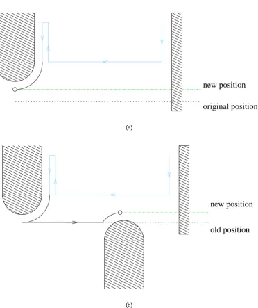
by an obstacle while executing theα segment of the U-shaped pattern. In Figure 2.16(b), the

side boundary the robot follows in theαsegment disappears. In Figure 2.16(c), the robot’s path

inβis obstructed by an obstacle. Figure 2.16(d) shows an unexpected non-collision in segment

β, where the robot does not encounter the side boundary as expected. In Figure 2.16(e), the

robot loses contact with the side boundary. This is distinct from the situation in Figure 2.16(b)

in that during the αsegment the robot is outside the covered portion of the cell, while during

segmentδit is not.

When the robot encounters any of the five events, it attempts to fully explore the new cell boundary. The maneuvers used depend on the event. The intervals associated with the current

cell are updated. After the cell boundary is completely explored, the algorithm searches the list

of placeholders H for any uncovered cells. Travelling between cells is done by moving into

each cell in between, and moving first in one direction, for example x, then the other direction,

y, in order to reach the next cell.

Unlike the zigzag (Figure 2.17), the U-shaped pattern contains retracing. This retracing is

added to include wall following on both side boundaries. This is because a contact sensing

robot cannot detect obstacles except when wall following. Therefore, if the robot is following a

zigzag pattern and an opening occurs as shown in Figure 2.18, the robot will miss it.

Acar et. al. introduced Morse decomposition [8, 9] for range sensing robots covering unknown

environments. Cell boundaries in Morse decomposition are critical points of Morse functions.

The decomposition is based on a roadmap method originally proposed by Canny [26, 27]. Given

a real-valued function h : Rm → R, its differential at p ∈ Rm is dhp = [_∂x∂h₁(p)· · ·_∂x∂h_m(p)]. A

point p∈_Rm_{is a critical point of a Morse function if} ∂h

∂x1(p)= · · · =

∂h

(32)

2.2 Cell decomposition 21 (a) (b) (c) (d) (e)

(33)

[image:33.595.227.342.482.681.2]

Figure 2.17: Compared to the pattern in Figure 2.15, a zigzag includes wall following on only one side boundary.

Figure 2.18: Contact sensing robots (as used inCCR) will miss an opening in the side boundary unless

(34)

surface normal

Figure 2.19: A cell boundary in Morse decomposition occurs at this position because the surface nor-mal of the obstacle is perpendicular to the sweep line.

(_∂x∂2h

i∂xj(p)) is non-singular. To put it more simply, a critical point occurs when the sweep line

encounters an obstacle whose surface normal is perpendicular to the sweep line. This definition

of criticality for cell decomposition is explained graphically in Figure 2.19. Figure 2.20 shows

an example of Morse decomposition.

By using surface normals as criticality, the environment is limited to differentiable functions

only. Therefore, polygons cannot be handled as their vertices are non-smooth boundary points.

To overcome this limitation in Canny’s roadmap, Acar et. al. use Clarke’s generalised

gradi-ents [33, 67] to calculate surface normals at these non-smooth boundaries [9]. The generalised

gradient of a point x is the set of vectors within the convex hull of the surface normals of the

adjacent smooth surfaces around x (see Figure 2.21). The generalised gradient can be used on

any point x that is not differentiable, given that the function is Lipschitz around x. A function

is locally Lipschitz for a bounded subset B if there exists a constant K such that

|f (x1)− f (x2)| ≤ K|x1−x2|

for all points x1and x2of B. However, since any function with a discontinuity is not Lipschitz

around the discontinuity, rectilinear environments such as those used in CCRare not covered by

Morse decomposition.

Critical points in Morse decomposition can be detected using omni-directional range sensors.

Given a robot is at point x, then the closest point on the surface of obstacle Ci to point x is c0

c0= arg min

c∈Ci

kx−ck

Now, let d(x) be the shortest distance between point x and the obstacle Ci. Then the gradient6

can be determined by

∇d(x) = x−c0

kx−c0k

(35)

Figure 2.20: Criticality of Morse decomposition occurs at the positions of the black dots in the diagram. The dotted lines are the cell boundaries. Three of the critical points have no cell bound-aries drawn through because free space is of zero width at those positions.

(36)

c0

x

∇di(x)

Figure 2.22: Detecting critical points in Morse decomposition.

This equation can be explained as follows. As c0 is a point on the surface of the obstacle Ci,

then x−c0is a vector which points from c0towards x. However, because c0is the closest point on the surface from x, it is thus normal to the obstacle surface. Division bykx−c0k turns the result into a unit vector.

The robot has detected a critical point if the gradient ∇di(x) is perpendicular to the sweep

line. Figure 2.22 explains how critical points can be detected by robots equipped with omni-directional range sensors.

The Morse decomposition is stored as a Reeb graph7_{, with the critical points as nodes.}

Fig-ure 2.23 shows the graph corresponding to the decomposition in FigFig-ure 2.20. Note that the

edges in the graph represent the cells in the decomposition.

Similar to CCR, Morse decomposition has an associated algorithm for creating the

decomposi-tion online. It also employs the U-shaped coverage pattern in Figure 2.15. The wall following

offered by the U pattern is needed because critical points occurring on the side boundary, such

as those in Figure 2.24, cannot be detected even with unlimited range sensors except when wall

following [8]. This is because the robot can only detect critical points of Morse functions if the

critical point is closest to the robot compared to all other points on the obstacle surface.

An event occurs whenever the robot encounters a critical point while following the U-shaped pattern. Figure 2.25 shows the two events defined in Morse decomposition. In Figure 2.25(a),

the robot is following the side boundary of the current cell when it encounters a critical point.

The next lap position is moved to where the critical point is. In Figure 2.25(b), the robot

encounters a critical point while moving along the length of the U-shaped pattern.

Information about uncovered cells is associated with nodes in the Reeb graph (ie the critical

points). When the robot finishes executing a U pattern which is interrupted by critical points,

(37)

26 Coverage navigation and path planning p1 p2 p3 p4 p8 p5 p6 p7

Figure 2.23: Reeb graph for the Morse decomposition in Figure 2.20.

[image:37.595.178.388.103.449.2]

critical points missed

(38)

[image:38.595.124.497.178.622.2]

2.2 Cell decomposition 27 new position original position (a) old position new position (b)

(39)

it first looks for uncovered cells at the last encountered critical point. If the critical point is

associated with two uncovered cells (eg in Figure 2.25(b)), the robot picks one of the cells

associated as the next cell to cover. If there are no uncovered cells associated with the last

encountered critical point, a depth-first search is performed on the Reeb graph. To travel to

the selected uncovered cell, the robot follows the Reeb graph and plans a path that passes through cells and critical points. The environment is fully covered when no uncovered cells are

associated with any of the nodes in the Reeb graph.

Although the starting point of this thesis is to investigate coverage with landmarks in

topologi-cal maps (Section 2.4), the method proposed ultimately creates a cell decomposition similar to

the split and merge concept in boustrophedon decomposition. However, unlike boustrophedon

decomposition, this thesis deals with coverage of unknown environments. CCR is especially

designed for robots with no range sensing ability. Similar to this thesis, Morse decomposition

is for range sensing robots working in more general unknown environments. Compared with

Morse decomposition, the method proposed in this thesis can handle a larger variety of

envi-ronments (rectilinear, polygonal and non-polygonal). Moreover, wall following on both side

boundaries is not needed due to the use of more general landmarks as criticalities, or events, of the decomposition. Since retracing is eliminated from the coverage pattern, the proposed

algorithm generates shorter coverage paths.

Boustrophendon decomposition was first published in a conference in 1997 [32], and later as a

journal paper in 2000 [30]. CCR was first published in 1999 [23]. Morse decomposition was

first published in 2000 [7, 10], and thus was developed in parallel with the work in this thesis,

which was also first published in 2000 [100, 101].

2.3 Grid map

In grid maps, environments are decomposed into a collection of uniform grid cells. This uniform

grid includes both free space and obstacles. Each cell contains a value stating whether an

obstacle is present. The value can either be binary or a probability [37]. Figure 2.26 shows an

example of a grid map.

The major advantage of this type of map is the ease in creating one. It is essentially an ar-ray containing occupancy information for each cell of the map. However, grid maps require

accurate localisation to create and maintain a coherent map [28, 95]. They also suffer from

ex-ponential growth of memory usage because the resolution does not depend on the complexity

of the environment [94]. Also, they do not permit efficient planning through the use of standard

(40)

[image:40.595.212.413.86.288.2]

2.3 Grid map 29

Figure 2.26: A grid map. Grid cells with obstacle present are shaded.

Grid based maps are the most widely used spatial representation for coverage algorithms. This

is due to the simplicity of marking covered areas in a grid map.

Zelinsky et. al. proposed an offline coverage algorithm [108] based on the distance transform

of a known grid map [58]. Figure 2.27 shows the distance transform of a simple environment

with one obstacle. Here, S represents the initial (or starting) position of the robot, and G is the

desired finishing position. The distance transform thus represents a wavefront that propagates from the goal cell G to the initial cell S . The algorithm for calculating the distance transform

is shown in Algorithm 2.2. Lines 1 to 3 shows the initialisation needed before the execution of

the main loop in lines 4 to 11. In line 1, the distance transforms (DT) of all cells in the grid

are set to -1, which mark the cells as unprocessed. Execution starts with the goal cell G, which

has a distance transform of 0 (lines 2 and 3). In each iteration of the main loop, unmarked cells

who are neighbours of marked cells are assigned a DT one higher than their neighbours’. This

continues until all cells in the grid map are marked.

Once the distance transform for the environment is calculated, the coverage path can then be

formed by selecting the neighbouring cell with the highest DT and is unvisited, starting from the

initial cell S . If two or more unvisited neighbours have the same transform, one of them is se-lected randomly. Figure 2.28 shows the coverage path generated for the example in Figure 2.27.

The algorithm for generating the coverage path is explained in Algorithm 2.3.

Unlike other coverage algorithms, this distance transform based method requires the selection

of a goal location.

Ulrich et. al. [97] also used a grid map for their online coverage algorithm. The algorithm

starts with an exploration of the boundary of the environment. Afterwards, the robot moves

(41)

30 Coverage navigation and path planning 13 13 S 12 12 12 11 11 11 10 10 10 9 8 9 9 9 9 9 9 9 9 8 8 8 8 8 8 8 8 5 4 7 7 7

7 7 7

7 7 7 7 7 7 6 6 6 6 6 6 5 5 5 5 5 5 4 4 4 4 4 4 6 6 6

4 4 4 4

7 7 7 7

6 6 6 6 6

5 5 5 5 5

[image:41.595.122.444.102.336.2]

4 4 4 4 4 4 3 3 3 3 3 3 3 3 3 3 3 3 1 1 2 2 2 1 1 G 1 2 2 1 1 1 2 2 2 2 2 2 2 2 2 2 2 3 3 3 3 3

Figure 2.27: Distance transform for the selection start position (S) and goal position (G). (Reproduced from [108]).

Algorithm 2.2 Distance Transform for a Grid Map Require: goal cell G

1: DT(all cells)← −1

2: DT(G)←0

3: n← 0

4: while there exists a cell c where DT(c)=-1 do 5: for all x such that DT(x)=n do

6: if y is a 8-neighbour or x and DT(y)=-1 then

7: DT(y)←n+1

8: end if 9: end for

10: n← n+1

11: end while

Algorithm 2.3 Coverage Path Planning using Distance Transform c←start cell

visited(all cells)←false

repeat

visited(c)←true

c←neighbouring cell with highest DT

(42)

2.3 Grid map 31

9 8 7 6 5 4 3 2 2 2 2 2 3 4

4 3 2 1 1 1 2 3 4 5 6 7 8 9

9 8 7 6 5 4 3 2 1 G 1 2 3 4

4 4 3 3 2 2 2 1 1 3 2 2 3 3 2 2 1 3 4 5 6 7 8 9 9 9 8 8 7 7 6 6 5 5 4 4 3 3

3 3 3 4

[image:42.595.155.470.89.316.2]

4 5 6 7 7 6 5 4 4 5 6 7 7 6 5 4 4 5 6 7 7 6 5 6 6 7 7 7 7 8 8 8 9 9 9 10 10 10 11 11 11 12 12 12 13 13 S

Figure 2.28: Coverage path generated from the distance transform. (Reproduced from [108]).

of travel is chosen. One of the criteria for the new direction is a high number of uncovered

grid cells. The algorithm also attempts to generate a path that ends successively with mutually perpendicular walls (see Figure 2.29). This is done so the robot can alternately re-calibrate the

x and y coordinates of its odometry estimation, with values obtained from the initial exploration

phase. Since only a partial map is available, it may not be possible for the robot to reach the

target wall in the chosen direction due to the presence of unknown obstacles. In this case, the

robot updates the grid map and then selects a new direction of travel again. The path planning

used in this work is a na¨ıve approach and results in highly redundant paths, as can be seen in

Figure 2.29.

Unlike the almost random approach taken by Ulrich et. al., Gabriely and Rimon tackle the

problem of coverage path planning on a partial grid map with a systematic spiral path. This

is achieved by following a spanning tree of the partial grid map [45]. Two different sizes of

grid cells are used. The smaller grid cell is the same size as the robot. Four of these smaller

grid cells then form a mega cell. These concepts are shown in Figure 2.30. The details of this

spanning tree approach is shown in Algorithm 2.4. The two parameters to the function STC

are the current cell x and its parent cell w. The algorithm is started by executing STC(NULL,

start cell). NULL is used for the parent cell because the start cell has no parent. A mega cell is old (line 1), if at least one of its four subcells is covered; otherwise, it is new (line 2). At

each mega cell, the robot picks a new direction of travel by selecting the first uncovered free

space mega cell in an anti-clockwise direction (line 3). A spanning tree edge is also grown

from the current mega cell to the new one (line 4). The algorithm is recursive (line 6), and the

(43)

[image:43.595.157.412.85.317.2]

start end

Figure 2.29: The robot path in the work of Ulrich et. al. is highly inefficient. The dotted line represents the path taken by the robot during boundary exploration, while the solid line represents the path taken during coverage. (Reproduced from [97]).

the robot along one side of the spanning tree (line 5) until it reaches the end of the tree (line

2), at which point it turns around to move along the other side of the tree (line 8). Figure 2.31

shows the spanning tree and the coverage path for the environment in Figure 2.30. Notice that

when coverage is completed, the robot returns to the same mega cell as the initial location.

Algorithm 2.4 Spiral spanning tree coverage STC(w,x)

1: Mark the current cell x as old

2: while x has a new obstacle-free 4-neighbour cell do

3: Scan for the first new neighbour of x in anti-clockwise order, starting with the parent

cell w. Call this neighbour y.

4: Construct a spanning-tree edge from x to y.

5: Move to a subcell of y by following the right-side of the spanning tree edges.

6: Execute STC(x,y).

7: end while

8: if x_,start cell then

9: move back from x to a subcell of w along the right-side of the spanning tree edges.

10: end if

Normally, cells in a grid map are square in shape and the same size as the robot. Oh et. al. proposed the use of a grid with triangular cells in their coverage algorithm instead [80] (see

Figure 2.32). The rationale behind using a triangular grid is that it has a higher resolution

com-pared to a rectangular one with similar sized cells. The use of alternative tiling arrangements to

increase resolution is well known in image processing [74]. Oh et. al. showed that this increase