An efficient and accurate MEMS accelerometer model with sense finger dynamics for applications in mixed technology control loops

An efficient and accurate MEMS accelerometer model with

sense finger dynamics for applications in

mixed-technology control loops

Chenxu Zhao, Leran Wang and Tom J. Kazmierski

University of Southampton, UK {

cz05r,lw04r,tjk

@ecs.soton.ac.uk

ABSTRACT

This contribution presents a novel MEMS accelerometer model implemented in VHDL-AMS. The model includes sense fin-ger dynamics, which allow accurate performance prediction of a MEMS accelerometer in a mixed-technology control loop. A distributed mechanical sensing element model is developed and the effect of the sense finger dynamics is an-alyzed. The sense finger dynamics might cause a failure of the Sigma-Delta control loop which is captured by the proposed model but cannot be correctly modeled using the conventional approach.

1.

INTRODUCTION

Micro-ElectroMechanical Systems (MEMS) require an inte-gration of mechanical and electrical elements. These two dis-parate parts of a MEMS system have traditionally been de-signed separately using different methodologies and tools in different energy domains. Although several approaches have been proposed to mixed technology modeling of such sys-tems [3], automated design methodologies for the whole in-tegrated system supporting mixed physical domains are lag-ging behind. Recent AMS hardware description languages such as VHDL-AMS [1] are designed to support digital, ana-log and mixed-signal systems but they cannot handle di-rectly partial differential equations that are often needed to model distributed mechanical parts.

Due to the relatively high resolution and low temperature sensitivity, capacitive accelerometers are widely used in var-ious industrial applications. Capacitive sensing of accelera-tion is also very well suited for applicaaccelera-tions that use closed-loop control systems [4]. The MEMS capacitive accelerom-eter detects the mechanical displacement of the proof mass which is proportional to the input acceleration and trans-lates it into an electrical signal, as the displacement of the proof mass changes the gap between the electrodes of ca-pacitors, leading to a change in capacitance which can be measured easily. In order to improve the performance of the accelerometer in terms of bandwidth, dynamic range and lin-earity [2], and to convert analog acceleration signals directly to a digital form, electromechanical Sigma-Delta modulation (SDM) feedback control is usually applied. The output of such an accelerometer system is a digital pulse stream whose density represents the input acceleration.

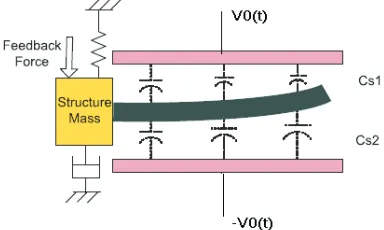
The accelerometer proof mass is usually equipped with sense fingers placed between capacitor plates to increase the total

capacitance variation when the proof mass moves (see Fig-ure 1). The main drawback of this arragement is that finger resonance may affect the performance of the electromechan-ical Sigma-Delta modulator [5]. Sense fingers might bend seriously and oscillate at their resonant frequency leading to a failure of the oscillation of the Sigma-Delta control loop. However, the conventional approach normally applied in simulations of such systems, where a 2nd order lumped Mass-Damper-Spring equation is used to model the mechan-ical sensing element, cannot capture the effect of the sense finger dynamics. That means a failure of the Sigma-Delta control loop, when the fingers resonate, cannot be predicted correctly unless a more accurate modeling technique is used.

Figure 1: Distributed model for mechanical sensing element

This paper proposes a distributed approach where the sense fingers are modeled as cantilever beams whose motion can be described by Partial Differential Equations(PDEs). Since VHDL-AMS does not support PDEs, a Finite Difference Ap-proximation (FDA) approach is applied to convert the PDE to a set of ODEs. Simulation results show that finger dy-namics can be captured accurately using only a few discrete sections to approximate all the cantilever beams combined into a single equivalent sense finger.

2.

CONVENTIONAL MEMS DIGITAL

AC-CELEROMETER MODELING

f(t) =Md

2_x

dt2 +D dx

dt +Kx (1)

where f(t) represents the input and feedback force, M is the mass of the proof-mass,xis the deflection of the proof-mass,DandKare damping coefficient and spring constant respectively.

Figure 2: 2nd-order electromechanical Sigma-Delta accelerometer

The gain blockKcvrepresents the signal pick-off from a

dif-ferential change in capacitance to a voltage. The lead com-pensator is required to ensure the stability of the Sigma-Delta feedback control loop. A clocked 1-bit quantizer is used for oversampling and generating pulse-density modu-lated digital signal. A pulse-density modulated feedback force is produced using the DAC. Figures 4 (a) and 5 (a) show simulation results of this model without accounting for finger dynamics. Figure 5 (a) indicates a correct opera-tion of the system where the pulse density is inversely pro-portional to the input signal. In reality however, the sense element is vibrating at this input frequency thus rendering the feedback excitation ineffective, causing an incorrect out-put and a failure of the system [5]. This scenario cannot be reflected by the conventional model.

3.

SENSE FINGER DYNAMICS

This section presents a more accurate approach to modeling the mechanical sensing element, which is distributed and can exhibit higher resonant modes. Such a model can be derived from the geometry of the sense electrode as illustrated in Figure 1. This is also a non-collocated system [5]. The feedback force is applied to the lumped mass(the root of the cantilever beam) and the electrostatic force is distributed along the length of the beam. Cs1 and Cs2 are the total

distributed differential capacitances between the beam and the electrodes. V0(t) is the excitation carrier voltage. The motion of the beam could be modeled by the following partial differential equation (PDE):

ρS∂

2_{y(x, t)}

∂t2 +CDI

∂5y(x, t)

∂x4∂t +EI

∂4y(x, t)

∂x4 =Fe(x, t) (2)

where y(x, t) is a function of time and position that rep-resents the deflection of the beam. E, I, CD,ρ, S are all

physical properties of the beam:ρis the material density,S

is the cross sectional area (W∗T),W andT are width and thickness of the beam, E represents the Young’s modulus which defines a material’s shearing strength,Iis the second moment of area which could be calculated byI=W T3/12,

EI is usually regarded as the flexural stiffness, CD is the

internal damping modulus, Fe(x, t) is the distributed

elec-trostatic force along the beam:

Fe(x, t) =

1 2εA[

V02

(d0−y(x, t))2 −

V02

(d0+y(x, t))2] (3)

whereεis the permittivity, A is the area of the electrode,d0

is the initial spacing between the beam and the electrode and V0 is the amplitude of the applied excitation carrier

voltage.

The boundary conditions of the cantilever beam are de-scribed by the following equations:

At root (x=0)

y(0, t) =z(t) (4)

∂y(0, t)

∂x = 0 (5)

At free end (x=l)

∂2y(l, t)

∂x2 = 0 (6) ∂3y(l, t)

∂x3 = 0 (7)

z(t) is the deflection of the structure mass which could be modeled by a 2nd order differential equation as Equation 1:

Md

2_z(t)

dt2 +D dz(t)

dt +Kz(t) =Ff eedback+Finput (8)

In order to implement the above equation in VHDL-AMS, a Finite Difference Approximation (FDA) is applied to convert PDEs to a series of DAEs. Firstly, the beam is divided into N segments. 5 segments are chosen in this design as this number has been found adequate to reflect a failure of the system when the beam resonates. The deflection of the beam is discretized as:

yn(t) =y(nx, t) n= 0,1,2...N (9)

So the partial derivatives wrt position can be eliminated from Equation 3 and replaced with:

∂yn(t)

∂x =

yn(t)−yn−1(t)

Hence, the cantilever PDE (Equation 3 is converted to a set of Ordinary Differential Equations:

ρSd

2_y n

dt2 + CDI

(x)4(

dyn+2

dt −4 dyn+1

dt + 6 dyn

dt (11)

−4dyn−1

dt + dyn−2

dt ) + EI

(x)4(yn+2−4yn+1+ 6yn −4yn−1+yn−2) = fen(t)

x (n= 0,1,2...N)

Equations for the border segments could be obtained from the boundary conditions. The complete, discretized dis-tributed model consists of 6 DAEs shown in the following VHDL-AMS code.

library IEEE PROPOSED;

use IEEE PROPOSED.ENERGY SYSTEMS.all; use IEEE PROPOSED.ELECTRICAL SYSTEMS.all; use IEEE PROPOSED.MECHANICAL SYSTEMS.all; library IEEE;

use IEEE.MATH REAL.all;

entity SENSING is generic(

dx: real:=1.4e-4/5.0; --length of each -- finger section E: real :=1.3e+11; --Young’s modulus I: real:=0.17e-24; --Moment of inertia rou: real:=2330.0; --Density

d0: real:=2.0e-6; --Initial gap

K: STIFFNESS:=100.0; --Spring stiffness D:DAMPING:=0.001; --Damping constant A:real:= 2.0e-6*1.4e-4/5.0; --Area of each

--section S:real:= 2.0e-6*1.0e-6;--Cross section area C:real:=0.01e-20;--Internal damping modulus

-- of finger M:MASS:=3.0e-7; --Lumped mass Kcv:real); --Signal pick-off gain port(

terminal STRUCTURE MASS: TRANSLATIONAL; terminal MID EL : ELECTRICAL);

end entity SENSING;

architecture BHV of SENSING is

--Distributed displacement of each segment--quantity y0,y1,y2,y3,y4:DISPLACEMENT;

--Distributed electrostatic force--quantity FE1,FE2,FE3,FE4:FORCE;

--Displacement of structure

mass--quantity x across F0 through STRUCTURE MASS to REF;

--Output

Voltage--quantity Vout across Iout through MID EL to electrical ref;

--Total distributed capacitances--quantity C1,C2:CAPACITANCE;

begin

--Electrostatic forces along the finger--FE1==0.5*8.85e-12*A*(9.0/((d0-y1)**2) -9.0/((d0+y1)**2)); FE2==0.5*8.85e-12*A*(9.0/((d0-y2)**2) -9.0/((d0+y2)**2)); FE3==0.5*8.85e-12*A*(9.0/((d0-y3)**2) -9.0/((d0+y3)**2)); FE4==0.5*8.85e-12*A*(9.0/((d0-y4)**2) -9.0/((d0+y4)**2));

--First segment displacement--y0==X;

--Second segment motion equation--E*I*(Y3-4.0*Y2+6.0*Y1-3.0*Y0)/dx**4+ ROU*S*Y1’DOT’DOT+C*(Y3’DOT-4.0*Y2’DOT+ 6.0*Y1’DOT-3.0*Y0’DOT)/dx**4==FE1/dx;

--Third segment motion equation--E*I*(Y4-4.0*Y3+6.0*Y2-4.0*Y1+Y0)/dx**4+ ROU*S*Y2’DOT’DOT+C*(Y4’DOT-4.0*Y3’DOT+ 6.0*Y2’DOT-4.0*Y1’DOT+Y0’DOT)/dx**4==FE2/dx;

--Fourth segment motion equation--E*I*(-2.0*Y4+5.0*Y3-4.0*Y2+Y1)/dx**4+ ROU*S*Y3’DOT’DOT+C*(-2.0*Y4’DOT+5.0*Y3’DOT-4.0*Y2’DOT+Y1’DOT)/dx**4==FE3/dx;

--Free-end segment motion equation--E*I*(Y4-2.0*Y3+Y2)/dx**4+ROU*S*Y4’DOT’DOT+ C*(Y4’DOT-2.0*Y3’DOT+Y2’DOT)/dx**4==FE4/dx;

--Structural mass motion equation--M*X’DOT’DOT+D*X’DOT+K*X==F0; --Differential Capacitances--C2==8.85e-12*A*(1.0/(d0+y0)+1.0/(d0+y1) +1.0/(d0+y2)+1.0/(d0+y3)+1.0/(d0+y4)); C1==8.85e-12*A*(1.0/(d0-y0)+1.0/(d0-y1) +1.0/(d0-y2)+1.0/(d0-y3)+1.0/(d0-y4)); --Output Voltage--Vout==Kcv*(C1-C2)/(C1+C2); end architecture BHV;

For this differential capacitive sensing element, the total dis-tributed capacitance between the middle sense finger and electrodes is:

Cs1(t) = εA

n

₁

d0−yn(t)

(12)

Cs2(t) = εA

n

₁

d0+yn(t)

(13)

where n is the number of the sections of the finger (5 sections in this model). The output voltage can be calculated as:

Vout(t) = Cs1−Cs2

Cs1+Cs2Kcv (14)

The gainKcvrepresents the signal pick-off from a differential

Like in the conventional model, the lowest resonant mode is caused by the dynamics of the structure mass, when the sense finger and lumped mass move together. The resonant frequency is approximatelyw0=

K/M where theKis the suspension spring constant andM is the total mass of the lumped mass and sense fingers. The higher resonant mode is related to the sense finger resonance, then the fingers bend significantly while the lumped mass has a small deflection. The resonant frequency could be calculated as that of the cantilever beam [5]:

ωi=α2iW

L2

E

12ρ (15)

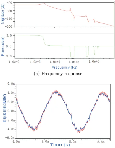
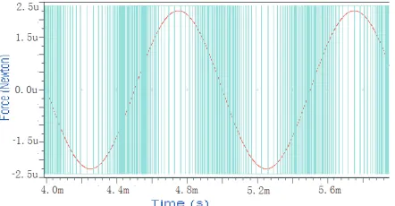
The finger dimensions in this design are: L= 140μm,W = 2μm,T = 1μm. The first and second resonant frequencies are 60KHz and 385KHz respectively. Figure 3 shows the frequency response of this model which agrees well with the calculation results.

The sense finger resonance could affect the performance of the Sigma-Delta control loop as fingers might bend seri-ously and oscillate at their resonant frequency which causes a breakdown of the Sigma-Delta control. As shown in Fig-ure 5 (b), fingers with the length L=200μm resonate and the Sigma-Delta control breaks down causing a fixed-density output waveform which does not reflect the input signal at all. The slight CPU time overhead related with the extra equations for finger dynamics is shown in the comparison between these two models in Table 1. SystemVision v.4 from Mentor Graphics was used to carry out the simulation experiments.

MODEL CPU TIME(SystemVision)

Conventional Model 9s 766ms

Distributed Model 21s 812ms

Table 1: CPU time comparison

4.

CONCLUSION

An accurate MEMS accelerometer model with sense finger dynamics has been developed and implemented in VHDL-AMS. The accelerometer operates in a high-sensitivity elec-trostatic Sigma-Delta control loop. Simulation results show that the proposed model correctly reflects the way in which finger dynamics affect the performance of the control loop. In contrast, the widely used conventional model of the ac-celerometer does not capture the well-known failure of the control loop when the system is excited with a frequency close to the sense finger resonance.

REFERENCES

[1] D.A.Teegarden, P.J.Ashendenm, and G.D.Peterson.The system designers guide to VHDL-AMS analogue, mixed-signal, and mixed-technology modelling. Morgan Kaufmann Publishers Inc, US, 10 Sep 2002.

[2] Y. Dong, M. Kraft, C. Gollasch, and W. Redman-White. A high-performance accelerometer with a fifth-order

sigma-delta modulator.JOURNAL OF

MICROMECHANICS AND MICROENGINEERING,

15:S22–S29, 2005.

(a) Frequency response

(b) Displacement of the lumped-mass (Blue) and average position of the beam (Red)

(c) Digital output bitstream

Figure 3: Simulation results for distributed model (L= 140μm)

[3] D. C. Hamill. Lumped equivalent circuits of magnetic components: The gyrator-capacitor approach.IEEE Trans. Power Electron, 8(2):97–103, Apr 1993.

[4] M. Kraft, C. Lewis, T. Hesketh, and S. Szymkowiak. A novel micromachined accelerometer capacitive interface.

Sensors & Actuators, A68/1-3:466–473, 1998.

(a) Frequency response of the conventional lumped model

(b) Frequency response of the distributed model

Figure 4: Frequency response of the models(L = 200μm)

(a) Output bitstream of the conventional model. The Sigma-Delta control loop works while in reality the con-trol breaks down. This behavior is incorrect.

(b) Output bitstream of the proposed model showing the fail-ure of the Sigma-Delta control loop at the finger resonant frequency. The proposed model correctly reflects this effect.