The Nordic Seas circulation and exchanges

(1)

University of Southampton Research Repository

ePrints Soton

Copyright © and Moral Rights for this thesis are retained by the author and/or other

copyright owners. A copy can be downloaded for personal non-commercial

research or study, without prior permission or charge. This thesis cannot be

reproduced or quoted extensively from without first obtaining permission in writing

from the copyright holder/s. The content must not be changed in any way or sold

commercially in any format or medium without the formal permission of the

copyright holders.

When referring to this work, full bibliographic details including the author, title,

awarding institution and date of the thesis must be given e.g.

AUTHOR (year of submission) "Full thesis title", University of Southampton, name

of the University School or Department, PhD Thesis, pagination

(2)

UNIVERSITY OF SOUTHAMPTON

The Nordic Seas Circulation and Exchanges

ELIZABETH HAWKER

A thesis submitted for the degree of Doctor of Philosophy

School of Ocean and Earth Science

(3)

UNIVERSITY OF SOUTHAMPTON

ABSTRACT

FACULTY OF ENGINEERING, SCIENCE & MATHEMATICS SCHOOL OF OCEAN & EARTH SCIENCES

Doctor of Philosophy

THE NORDIC SEAS CIRCULATION AND EXCHANGES

Elizabeth Hawker

The Nordic Seas provide the main oceanic connection between the Arctic and the deep global oceans via dense overflows between Greenland and Scotland, into the North Atlantic. An understanding of the circulation and exchanges of this region is vital for any consideration of the implications of high latitude climate change to variability in the Atlantic thermohaline circulation and consequences for regional (European) climate.

This thesis makes use of a unique data set of near synoptic hydrographic and LADCP (lowered acoustic Doppler current profiler) measurements across the entire region during summer 1999. The box inverse method is applied to this hydrographic data, using computed geostrophic velocities referenced to detided LADCP measurements. The full summer Nordic Sea flux field (volume, heat and freshwater) is quantified, studying both the exchanges across the openings to the Nordic Seas, and the interior circulation. The total volume transports imply an inflow of 1.3!±!0.5!Sv to the Nordic Seas from the Arctic Ocean, and a net export of 1.2!±!0.5!Sv across the Greenland!-!Scotland Ridge into the North Atlantic. Within the Nordic Seas 4.0!±!1.3!Sv of the warm saline inflow (s0!<!27.8) are converted to more dense waters, with the majority of the transformation (and ocean!

-!atmosphere heat loss) occurring over the southern part of the Nordic Seas. The total heat convergence within the Nordic Seas is 137!±!44!TW, giving an average flux of 51!±!16!W!m–2_{, and}

the net input of freshwater to the Nordic Seas is 0.059!±!0.019!Sv.

(4)

List of Figures

Figure 1.1: Latitudinal profiles of net incoming short-wave radiation, outgoing long-wave radiation, and the net radiative heating of the earth (Bryden and Imawaki, 2001).

4

Figure 1.2: Components of the atmosphere and ocean energy transports required to balance the net radiative heating of the earth following Figure 1.1 (Bryden and Imawaki, 2001).

4

Figure 1.3: Map of the Arctic Region using the International Bathymetric Chart of the Arctic Ocean (IBCAO) (Jakobsson et al., 2000).

5

Figure 2.1: Bathymetry and geographic features of the Nordic Seas. 38 Figure 2.2: Bathymetry and geographic features of the Greenland - Scotland Ridge and the Northern

North Atlantic.

39

Figure 2.3: Schematic showing the general circulation of the Nordic Seas (from Fogelqvist, 2003). 39 Figure 2.4: Annual mean sea level pressure from NCEP / NCAR Reanalysis data provided by the

NOAA-CIRES Climate Diagnostics Center, Colorado, U.S.A.

40

Figure 2.5: High resolution sea ice maps of the Arctic Ocean derived from satellite (passive microwave) sensors (DMSP-SSM/I) (Kaleshcke et al., 2001).

40

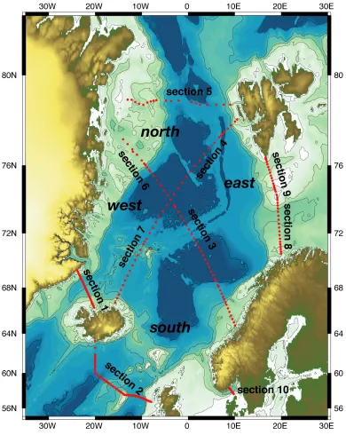
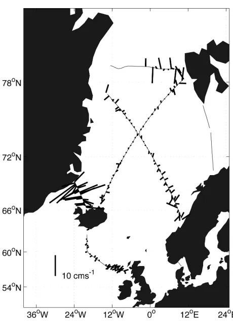
Figure 3.1: The Nordic Seas with station pair positions in red, showing the setup of boxes for the inverse calculation.

58

Figure 3.2: Hydrographic stations occupied during the individual cruises. 59 Figure 3.3: Comparison between the Egbert and Kowalik tidal models at two sites within the Nordic

Seas.

60

Figure 3.4: Station positions off the East Greenland coast on cruise JR44 showing the geographic locations of stations 042 and 043 in particular.

61

Figure 3.5: Geostrophic velocity (cm!s-1_{) for section 6.} ₆₁

Figure 4.1 87

Figure 4.2: Average tidal velocity (cm!s-1_{) over the duration of the hydrographic cast, applied as a}

barotropic correction to the on station WT and BT LADCP profiles.

88

Figure 4.3: Contoured section of the LADCP velocity field (cm!s-1_{) for Denmark Strait.} ₈₉

Figure 4.4: Contoured section of the LADCP velocity field (cm!s-1_{) across Fram Strait.} ₉₀

Figure 4.5: Contoured section of the LADCP velocity field (cm!s-1_{) for the Greenland to Norway}

section.

91

Figure 4.6: Contoured section of the LADCP velocity field (cm!s-1_{) for the Iceland to Svalbard section.} ₉₂

Figure 4.7: The differences (cm!s-1_{) between the WT and BT near bottom velocities (left panel) and}

the normal probability plot (right panel).

93

Figure 4.8: Velocity profiles for station pair 81 at 68.1°N 6.5°E in the Norwegian Sea. 93 Figure 4.9: Cumulative volume transports (Sv) from shipboard ADCP data and LADCP data in the

upper 500!m of the water column for the Iceland to Scotland section.

94

Figure 4.10: Long term mean Sea Level Pressure for September (millibars), for 1968 - 1996. 94 Figure 4.11: Mean Sea Level Pressure for September 1999 (millibars). 95 Figure 4.12: Anomaly in Sea Level Pressure (millibars) for September 1999 from the long term mean

(Septembers 1968 – 1996).

95

Figure 5.1a: Contoured potential temperature (°C) section across Denmark Strait. 130 Figure 5.1b: Contoured salinity section across Denmark Strait. 131 Figure 5.1c: q!/!S diagram (potential temperature / salinity plot) for the Denmark Strait section. 132 Figure 5.2a: Contoured potential temperature (°C) section across the Barents Sea Opening. 133 Figure 5.2b: Contoured salinity section across the Barents Sea Opening. 134 Figure 5.2c: q!/!S diagram (potential temperature / salinity plot) for the section across the Barents Sea

Opening.

135

(8)

Figure 5.3c: q!/!S diagram (potential temperature / salinity plot) for the section across Fram Strait. 138 Figure 5.4a: Contoured potential temperature (°C) section across the Skagerrak. 139 Figure 5.4b: Contoured salinity section across the Skagerrak. 140 Figure 5.4c: q!/!S diagram (potential temperature / salinity plot) for section across the Skagerrak. 141 Figure 5.5a: Contoured potential temperature (°C) section for the Greenland to Norway section. 142 Figure 5.5b: Contoured salinity section for the Greenland to Norway section. 143 Figure 5.5c: q!/!S diagram (potential temperature / salinity plot) for the section from Greenland to

Norway.

144

Figure 5.6a: Contoured potential temperature (°C) section for the Iceland to Svalbard section. 145 Figure 5.6b: Contoured salinity section for the Iceland to Svalbard section. 146 Figure 5.6c: q!/!S diagram (potential temperature / salinity plot) for the Iceland to Svalbard section. 147 Figure 5.7a: Contoured potential temperature (°C) section for the Iceland to Scotland section. 148 Figure 5.7b: Contoured salinity section for the Iceland to Scotland section. 149 Figure 5.7c: q!/!S diagram (potential temperature / salinity plot) for the Iceland to Scotland section. 150 Figure 5.8: Contoured section of the initial velocity field (cm!s-1_{; LADCP referenced geostrophy) for}

Denmark Strait.

151

Figure 5.9: Contoured section of the initial velocity field (cm!s-1_{; referenced geostrophy) across the}

Barents Sea Opening

152

Figure 5.10: Contoured section of the initial velocity field (cm!s-1_{; LADCP referenced geostrophy)}

across Fram Strait.

153

Figure 5.11 Contoured section of the initial velocity field (cm!s-1_{; referenced geostrophy) across the}

Skagerrak.

154

Figure 5.12: Contoured section of the initial velocity field (cm!s-1_{; LADCP referenced geostrophy) for}

the Greenland to Norway section.

155

Figure 5.13: Contoured section of the initial velocity field (cm!s-1_{; LADCP referenced geostrophy) for}

the Iceland to Svalbard section.

156

Figure 5.14: Contoured section of the initial velocity field (cm!s-1_{; referenced geostrophy) for the}

Iceland to Scotland section.

157

Figure 5.15: Ekman volume transports (Sv) on station pair positions. 158

Figure 5.16: Summer mean windstress field (N!m-2_). ₁₅₈

Figure 5.17: Full depth transports (Sv) across each section used to form the inverse boxes calculated from the initial velocity field.

159

Figure 5.18: Cumulative sum of the percentage of total variance for each solution degree of the standard model.

159

Figure 5.19: Condition number for each solution degree of the standard model. 160 Figure 5.20: Eigenvalues for each solution degree of the standard model. 160 Figure 5.21: Nondimensional norm of residual versus nondimensional norm of solution. 161 Figure 5.22: Reference velocities (cm!s-1_{) from the standard solution for each station pair.} ₁₆₁

Figure 5.23: Effective diapycnal velocities(x!10-4_!_cm_!_s-1_{) from the standard solution for volume and}

salinity (layer interfaces 1 to 13) and temperature (layer interfaces 6 to 13).

162

Figure 5.24: Norms of solution vector (cm!s-1_{) for each solution degree of the standard model.} ₁₆₂

Figure 5.25: Diagonal of the observation resolution matrix for the standard solution. 163 Figure 5.26: Diagonal of the solution resolution matrix for the standard solution. 163 Figure 5.27: Full depth volume transports (Sv) across each section, calculated from the standard

solution and further adjusted for zero net volume flux in each box.

164

Figure 5.28: Volume transports (Sv) in layers for each station pair, calculated from the standard solution and further adjusted for zero net volume flux in each box.

165

Figure 5.29: Total heat fluxes across the northern and southern boundaries of the Nordic Seas, and total heat flux convergence (TW) over the region.

166

Figure 5.30: Total freshwater fluxes across the northern and southern boundaries of the Nordic Seas, and total freshwater divergence over the region.

166

Figure 5.31: Interior diapycnal velocities (106_!_m_!_s-1_{) and associated diapycnal volume transports}

(106_!_m3!_s-1_{) for each box.}

167

(9)

Figure 5.35: Cumulative volume transports (Sv) across the Skagerrak. 171 Figure 5.36: Cumulative volume transports (Sv) for the Greenland to Norway section. 172 Figure 5.37: Cumulative volume transports (Sv) for the Iceland to Svalbard section. 173 Figure 5.38: Cumulative volume transports (Sv) for the Iceland to Scotland section. 174 Figure 5.39 Circulation scheme for the Nordic Seas (surface and mid-depth) based on results from the

standard inverse model.

175

Figure 6.1: The magnitude of the formal errors in volume transport (Sv) for each station pair. 189 Figure 6.2: Full depth volume transports (Sv) with errors, for each section, calculated from the

standard solution and further adjusted for zero net volume flux in each box.

189

Figure 7.1: Map of the Nordic Seas showing the positions of the winter reoccupations of the summer JR44 stations, the five stations described in section 7.2, and the Svinøy and Greenland to Norway sections.

211

Figure 7.2: Potential temperature and salinity profiles for stations occupied in both summer and winter.

212

Figure 7.3: Plot of potential temperature and salinity, with contoured isopycnals, for winter stations in the central Greenland Sea.

213

Figure 7.4: Potential temperature and salinity profiles from stations occupied in the central Greenland Sea during winter 2000.

213

Figure 7.5: The mean profiles of temperature and salinity observed on stations occupied in the central Greenland Sea during winter 2000.

214

Figure 7.6: Comparison of the mean profiles of temperature and salinity on stations occupied in the central Greenland Sea during summer 1999 and winter 2000.

214

Figure 7.7: Annual cycle in Atmosphere - Ocean Heat fluxes per unit area (W!m-2_{) over both the}

Nordic Seas region and the individual inverse boxes.

215

Figure 7.8: Annual cycle in total Atmosphere - Ocean Heat fluxes (TW) over both the Nordic Seas region and the individual inverse boxes.

215

Figure 7.9: Potential temperature and salinity profiles for stations on the ‘winter’ Greenland to Norway section.

216

Figure 7.10: Mean velocities (cm!s-1_{) of the PIMMs floats deployed in ice against latitude.} ₂₁₇

(10)

List of Tables

Table 2.1a: Atlantic Waters of the Nordic Seas. 32

Table 2.1b: Polar Waters of the Nordic Seas. 33

Table 2.1c: Intermediate Waters of the Nordic Seas. 34

Table 2.1d: Deep Waters of the Nordic Seas. 35!/!36

Table 2.1e: Overflow Waters of the Nordic Seas. 37

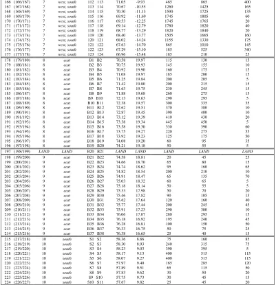
Table 3.1: Station Pairs used to create the north, south, east and west boxes. 55!/!56!/!57

Table 4.1: Flux errors due to seasonality in the volumes of the isopycnal layers. 65 Table 4.2: Layers defined by s0, s1 and s2 surfaces, with mean layer depth and thickness. 67

Table 5.1: Conventions used in this thesis to identify water masses. 98

Table 5.2: Layers defined by s0, s1 and s2 surfaces, with area-weighted layer-average potential temperature

(°C) and salinity.

100

Table 5.3: Ekman Volume (Sv), Temperature (Sv °C) and Salinity (Sv psu) Transports calculated from the SOC and HR summer average climatologies.

105

Table 5.4: Air-Sea Heat fluxes per unit area (Wm-2_{), and total (TW), over both the Nordic Seas region and}

the inverse boxes.

107

Table 5.5: Transport estimates (Sv) for the Nordic Seas, from the literature, the initial velocity field, and the standard solution of the inverse model.

128

Table 5.6: Heat Flux estimates (TW) for the Nordic Seas, from the literature, the initial velocity field, and the standard solution of the inverse model.

129

Table 5.7: Full depth volume transports (Sv) for each of the inverse boxes and the entire Nordic Seas region from the initial state of the standard model.

110

Table 5.8: Details of the constraints applied in the standard inverse model. 112

Table 5.9: Mean, peak and standard deviation of the barotropic corrections (cm!s-1_{) to the reference}

velocities from the standard solution.

114

Table 5.10: Mean, peak and standard deviation of the corrections (x!10-5_cm!s-1_{) to the effective diapycnal}

velocities from the standard solution.

115

Table 5.11: Volume transports (Sv) for each section, and for each layer, from the standard solution. 118 Table 5.12: Volume transports (Sv) summarised from Table 5.12, for exchanges between the Nordic Seas and

the North Atlantic across the Greenland-Scotland Ridge, across the Greenland-Norway section, and into the Arctic Ocean through Fram Strait and the Barents Sea Opening.

127

Table 6.1: a priori errors in the volume conservation equations, and layer mean and standard deviations of potential temperature and salinity for each box used in the inverse calculation.

178

Table 6.2: Specifications of alternative models to test inverse and oceanographic sensitivity. 180 Table 6.3: Volume Transport estimates (Sv) and Heat Fluxes (TW) for the Nordic Seas for the standard

solution and the alternative model runs.

187!/!188

Table 6.4: Summary of errors in volume flux from sensitivity tests. 185

Table 7.1: Atmosphere-Ocean Heat fluxes per unit area (Wm-2_{), and total (TW), over both the Nordic Seas}

region and the individual inverse boxes.

194

Table 7.2: Station Pairs on the Greenland to Norway ‘winter’ section. 195

Table 7.3: Volume transports (Sv) across the Greenland to Norway section, for summer and winter, and for each layer.

200

Table 7.4: Net errors derived from the net volume fluxes (Sv) and heat fluxes (TW) across the Greenland to Norway section from sensitivity tests.

(11)

Graduate School of the

Southampton Oceanography Centre

This PhD dissertation by

Elizabeth Hawker

has been produced under the supervision of the following persons

Supervisor/s Dr Sheldon Bacon and Professor Harry Bryden

Chair of Advisory Panel Professor John Murray (to July 2003)

Professor Peter Killworth (from July 2003)

(12)

DECLARATION OF AUTHORSHIP

I, ………..,

declare that the thesis entitled

……….………

and the work presented in it are my own. I confirm that:

ß this work was done wholly or mainly while in candidature for a research degree at this

University;

ß where any part of this thesis has previously been submitted for a degree or any other

qualification at this University or any other institution, this has been clearly stated;

ß where I have consulted the published work of others, this is always clearly attributed;

ß where I have quoted from the work of others, the source is always given. With the exception of

such quotations, this thesis is entirely my own work;

ß I have acknowledged all main sources of help;

ß where the thesis is based on work done by myself jointly with others, I have made clear exactly

what was done by others and what I have contributed myself;

ß none of this work has been published before submission

Signed: ………..

(13)

Acknowledgements

I would like to formally thank NERC for the use of ARCICE data from JR44 and JM3/2000;

Sheldon Bacon and Margaret Yelland as the PSO’s on JR44; Peter Wadhams, Jan Backhaus and

Else Nøst Hegseth as the PSO’s on JM3; and Stuart Cunningham (Southampton Oceanography

Centre) for D242 data, Ursula Schauer (Alfred-Wegener-Institut) for ARKTIS XV/3 data and

Johann Blindheim for data from the Svinøy section. My thanks also to the officers, crews and all

cruise participants, without whose efforts this thesis would not exist.

My sincere thanks to my supervisors Sheldon Bacon and Harry Bryden, and to my advisory panel;

but particularly to Sheldon for his insight and encouragement, and for giving me a long rein.

Thanks to the crew and officers of the RRS James Clark Ross who were there the first time I went

to sea, and to all shipmates on that and subsequent cruises - for reminding me what this is for.

Thanks also to all in the hydrography team of the James Rennell Division; to Alberto Garabato and

Cecilie Mauritzen for helpful discussion; to Rebecca Woodgate and Peter Rhines for guidance

during my exchange to the University of Washington, Seattle, and afterwards; and to Deb

Shoosmith for her continued encouragement.

I am indebted to Sheldon and Margaret Yelland who quite literally gave me a home in Southampton,

and whose company and friendship gave my time here purpose. Thanks to my housemates; Anna

who understood about the PhD, and Chess who understood the urge to escape Southampton and

who was with me during the darkest hours. Thanks to SV Tenacious and all who sail on her, for

showing me there are other ways to ‘go to sea’. Similarly, of course, thanks to all those who have

kept me company on a hilltop or mountainside, for showing me ‘there are other mountains’ than

those down south. Finally, my thanks to Mark Brandon, for his support, for being there the first

time I went south, and for understanding.

And it goes without saying, I am forever grateful for the love and support of my parents, even when

(14)

for Mark Brandon,

who shared his South with me

One does not discover new lands without consenting to lose sight of the shore for a very long time.

(15)

Chapter One

Introduction

‘Begin at the beginning,’ the King said, gravely, ‘and go on till you come to the end: then stop.’

Lewis Carroll

(16)

Chapter 1: Introduction 2

The primary motivation for studying ocean circulation is to understand its importance to the climate

system, particularly with respect to modern concern over climate change. The Earth’s surface

receives an uneven distribution of energy from the sun, with a greater influx of solar radiation at low

latitudes (Figure 1.1). The global oceanic and atmospheric circulations balance this meridional bias

by a transport of heat from low to high latitudes (Figure 1.2; Bryden and Imawaki, 2001).

The meridional overturning circulation (MOC) of the North Atlantic releases considerable amounts

of heat to the atmosphere as warm subtropical waters are transported to high latitudes where they are

transformed to cold (and so more dense) waters. This results in a southward flow of deep cold water

and a northward ocean heat transport at all latitudes in the Atlantic Ocean (Bryden and Imawaki,

2001). This northward heat transport (even south of the equator) is peculiar to the Atlantic Ocean,

and emphasises the influence that the high latitudes of the Nordic Seas and Arctic Mediterranean

have on the global ocean circulation.

The North Atlantic Current (NAtlC) carries warm Atlantic waters from the subtropics to higher

latitudes within the North Atlantic. It is cooled and freshened as it splits to follow one pathway

through the subpolar gyre and another through the Nordic and Polar Seas (Figure 1.3) to the north

(Mauritzen, 1996a). The principal transformations of the Atlantic waters occur in the seas of the

Arctic Mediterranean, where they lose heat and become more dense. The intermediate waters which

then overflow the Greenland-Iceland-Scotland ridge contribute to the source waters of North

Atlantic Deep Water (NADW). The importance of understanding the variability and formation

mechanisms of these overflows has been emphasised by studies of the North Atlantic which have

shown how both the strength and structure of the meridional overturning are affected by the

downstream development of the overflows (Saunders, 2001; Wood et al., 1999).

The data which provided the framework and motivation for this PhD were collected under the

auspices of ARCICE (Arctic Sea Ice and Environmental Variability), a thematic programme of the

UK Natural Environment Research Council (NERC). The core cruise from the ARCICE

programme, JR44 (CATS-MIAOW), was the most extensive modern major synoptic survey to be

made within the Nordic Seas, and the data provide a unique set of near synoptic hydrographic and

LADCP (lowered acoustic Doppler current profiler) measurements across the entire region during

summer 1999. The box inverse method is applied here, to this data together with supplementary

hydrographic data, using geostrophic velocities referenced to detided LADCP measurements where

possible. A further ARCICE cruise (JM3) also collected winter data over a reduced region of the

Nordic Seas. This data set is used to characterise the winter circulation and to contrast it to the

summer circulation.

The Nordic Seas provide a substantial part of the headwaters of the Atlantic thermohaline

circulation. The water mass transformations within them provide a direct link between the

atmosphere and ocean and are of consequence for the stability of the global thermohaline

(17)

sealers and whalers, and earlier (e.g. Koch, 1945), and there have been oceanographic studies since

the era of Knudsen (1899) and Nansen (1902). However, while many of the key processes involved

in the ventilation, pathways and overflows of the Nordic Seas are quantified and understood, there

remain many outstanding questions, and an overall understanding of the components of the Nordic

Seas system is yet to be established. To this end, this thesis quantifies the full Nordic Sea flux field

(volume, heat and freshwater), thus determining the exchanges between the Nordic Seas and the

Arctic Ocean to the north, the Barents Sea to the east, and North Atlantic to the south, via the North

Atlantic Current inflow and the Denmark Strait and Iceland-Scotland overflows. This is the first

study to be able to make use of synoptic hydrographic data across the entire region with concurrent

direct velocity measurements on most sections; and can therefore provide a new estimate of the

long-term mean summer fluxes and exchanges. The winter data also allow a winter circulation to be

constructed, suggesting how the summer mean field might be extrapolated to provide an estimate of

the ‘true’ annual mean flux field.

The structure of this thesis is as follows: Chapter 2 gives a general overview to set the work in

context and outlines the aims in view of the outstanding questions concerning the circulation of the

Nordic Seas. Chapters 3 and 4 give detailed descriptions of the data and methods used for this

study. The main results are presented in Chapter 5, which describes the summer circulation and

fluxes of the Nordic Seas. A study of the sensitivity of the inverse model and a discussion of errors

are the subject of Chapter 6. A discussion of the variability of the circulation and fluxes of the

Nordic Seas is made in Chapter 7, with reference to winter hydrographic data and the general ocean

climate. Chapter 8 summarises the conclusions of this thesis and briefly considers the future of

(18)

[image:18.595.216.450.114.336.2]

Figure 1.1: Latitudinal profiles of net incoming short-wave radiation, outgoing long-wave radiation, and the net radiative

heating of the earth (Bryden and Imawaki, 2001). The latitudinal scale is stretched so that it is proportional to the radius of

the earth. Q is the incoming short wave solar radiation, a is the albedo of the Earth, E is the outgoing long wave black body radiation, and R is the net radiation balance.

Figure 1.2: Components of the atmosphere and ocean energy transports required to balance the net radiative heating of

the earth following Figure 1.1 (Bryden and Imawaki, 2001). The total energy transport is that required to balance the net

radiative heating/cooling of the earth following Figure 1.1. The standard atmospheric energy transport is here divided into

the dry static atmospheric energy transport and the latent heat transport, because the latent heat transport is fundamentally

a joint atmosphere-ocean process as the atmospheric water vapour transport is balanced by an opposing oceanic freshwater

transport. The ocean heat transport is determined by integrating over the oceans the spatial distribution of

atmosphere-surface heat exchange calculated by subtracting the atmospheric energy transport divergence from the radiative heating at

[image:18.595.164.486.453.659.2]

(19)

Figure 1.3: Map of the Arctic Region using the International Bathymetric Chart of the Arctic Ocean (IBCAO)

(20)

Chapter Two

Overview

2.1 Introduction 7

2.2 Topography 7

2.3 Climate 9

2.3.1 Ocean Circulation 9

(i) General Circulation 9

(ii) Deep water formation 12

(iii) Variability 14

(iv) Circulation of the Arctic Ocean and Barents Sea 16

2.3.2 Atmosphere 18

2.3.3 Ice 19

2.3.4 Freshwater 21

2.4 Circulation Hypotheses 23

2.4.1 Atlantic Waters 23

2.4.2 Polar Waters 24

2.4.3 Intermediate Waters 24

2.4.5 Overflow Waters 26

2.4.6 DSOW formation mechanisms 27

2.5 High Latitude Climate Change 28

(21)

Chapter 2: Overview 7

2.1 Introduction

The Nordic Seas provide the main oceanic connection between the Arctic and the deep global

oceans via the exchanges with the North Atlantic across the Greenland-Scotland Ridge. The inflow

of warm, salty Atlantic waters and the outflow of ice and cold, fresh Arctic waters form two major

components of the Nordic Sea circulation, and influence the long-term variability of the overflows

into the North Atlantic. An understanding of the circulation and exchanges of the Nordic Seas is

vital for any consideration of the implications of high latitude climate change to variability in the

Atlantic thermohaline circulation and consequences for regional (European) climate.

This chapter gives a general overview to set the work of this thesis in context. The outstanding

questions concerning the circulation of the Nordic Seas reveal the impetus for this thesis, the aims of

which are outlined at the end of this chapter.

2.2 Topography

Oceanic topography influences the circulation, both by restricting exchanges and steering flow. The

study of the Nordic Seas (Figure 2.1) has, since before the time of Nansen, been confused by the use

of different terminology to describe geographical features and define water masses. For

Helland-Hansen and Nansen (1909) discussion of the Norwegian Sea included the waters of the Greenland,

Iceland and Norwegian Seas. These have also been aptly referred to as the ‘GIN Seas’ (Aagaard

and Carmack, 1989). Today they are known collectively as the Nordic Seas (Hurdle 1986), and

together with the Arctic Ocean, form the Arctic Mediterranean. Even today, however, their status is

contentious; whether to be regarded as the northern marginal seas of the Atlantic, or the southward

‘Atlantic sector’ extension of the Arctic?

The Greenland-Scotland Ridge itself (Figure 2.2) was discovered by various expeditions in the late

1800s (for overview, see Bacon, 2000). In particular, Denmark Strait, the part of the ridge between

Greenland and Iceland, was identified by soundings made by the Royal Danish Navy from 1877 to

1879. The presence of a ridge had been inferred by contemporary oceanographic expeditions which

identified subsurface ‘warm’ and ‘cold’ areas to the south and north of Iceland respectively. It

effectively acts as a dam to the deep waters of the Arctic, but allows exchanges of surface and

intermediate waters through various gaps. Denmark Strait and the Faroe Bank Channel (the

southward extension of the Faroe-Shetland Channel between the Faroe Islands and Scotland),

provide the deepest connections with sill depths of 600!m and 850!m respectively, while the

Iceland-Faroes ridge is cut by four ‘notches’ with sill depths of less than 450!m (Meincke, 1983).

The Greenland-Scotland Ridge constitutes a physical barrier between the Nordic Seas and Arctic

Ocean to the north, and the Atlantic Ocean to the south. As such, it restricts the exchanges of

(22)

Chapter 2: Overview 8 the north and the south of the ridge were noted as far back at the late 1800s. It may therefore be

more reasonable to consider the Nordic Seas as the southerly extension of the Arctic rather than

within the northern margins of the Atlantic.

The individual sub-basins of the Nordic Seas are defined by the submarine topography (Figure 2.1).

The Iceland Sea (~1800!m in depth), between Greenland, Iceland and the island of Jan Mayen, is

bounded by the Greenland-Iceland ridge to the south, and the Jan Mayen Fracture Zone to the north.

The Norwegian Sea is separated into the Norwegian (~3600!m in depth) and Lofoten (~3200!m in

depth) Basins and further north, extends east of the Knipovich Ridge towards Fram Strait. The

Greenland Sea is separated from the Norwegian and Iceland Seas by the Mohns Ridge and the Jan

Mayen Fracture Zone, respectively. The Mohns Ridge has numerous traverse gaps, some of which

are very important in the exchange of waters between and within basins, such as the broad saddle

(~2400!m depth) at ~75°30’N. The western depression of the Iceland Sea and the southern

depression of the Greenland Basin are connected (at a depth of ~1600!m) between the Greenland

continental slope and the westernmost portion of the Mohns Ridge by the Greenland!-!Jan Mayen

Gap. A shallow shelf leads east from the Nordic Seas into the Barents Sea, between Norway, Bear

Island and Svalbard. To the south of Bear Island lies Bjørnøyrenna, a channel with a maximum

depth of ~500!m. Storfjordrenna lies to the north of Bear Island, a channel with depth of ~300!m,

which shoals to the east, and is blocked by Svalbard to the north.

Fram Strait, between Greenland and Svalbard, provides the deep connection (sill depth of 2600!m)

between the Nordic Seas and the Arctic Ocean. The Arctic Ocean itself is a semi-enclosed ocean

(Figure 1.3). Its connections to the global oceans, apart from Fram Strait, are restricted to

exchanges with the North Atlantic through the Barents Sea (~250!m depth) via the Nordic Seas, and

the Canadian Archipelago (~200!m depth); and exchanges with the Pacific through the Bering Strait

(50!m depth). The Arctic Ocean is most simply considered to comprise of the Arctic Shelf Seas and

two deep basins; the Canadian basin (maximum depth of ~3800!m) and the Eurasian basin

(maximum depth of 4200!m) divided by the Lomonosov Ridge (sill depth of ~1400!m). The

shallow continental shelf regions make up as much as ~53!% of the entire area of the Arctic Ocean

(Jakobsson, 2002), compared to a range of 9.1 to 17.7!% for the remainder of the global oceans,

implying that its circulation may be particularly sensitive to sea level changes. The physical

restrictions of Bering Strait and the Canadian Archipelago mean the principal exchanges between

the Arctic and the global oceans occur across the Greenland-Scotland ridge system.

The Nordic Seas are also connected to the North Atlantic via the North Sea and English Channel

(Figure 2.2). The North Sea is a shallow (~100!m) marginal shelf sea bounded by the landmasses of

the United Kingdom and continental Europe. The only deep connection between the Nordic Seas

and the North Sea is a continental shelf depression called the Norwegian Trench. The deeper parts

of this follow the Norwegian coast into the Skagerrak (maximum depth of 710!m) and onwards into

(23)

Chapter 2: Overview 9 Within the North Atlantic, to the south of the Greenland-Scotland Ridge, the Irminger Basin off the

east coast of Greenland is separated from the Iceland basin by the Reykjanes Ridge, and further to

the east the Rockall-Hatton Plateau separates these basins from the Rockall Trough. Exchanges

between the Irminger and Iceland basins (between the western and eastern North Atlantic) are

limited, with the deepest passage being through the Charlie-Gibbs Fracture Zone.

2.3 Climate

The oceanic and atmospheric circulations of the Nordic Seas, together with the cryosphere, form

major components in the high-latitude climate system.

2.3.1 Ocean Circulation

A schematic of the oceanic circulation of the Nordic Seas is illustrated in Figure 2.3. Although the

broad features (inflows, overflows, boundary currents, basin-scale gyre circulations) are relatively

well understood, the specific details of the interior circulation, in particular, are not yet well

determined. The general oceanic circulation of the Nordic Seas is characterised by a surface inflow

of Atlantic Water towards the Arctic (via Barents Sea and Fram Strait) and a surface outflow of

cold, fresh water from the Arctic to the North Atlantic, separated by cyclonic gyres in the Greenland

and Norwegian Seas (Hopkins, 1991).

(i) General Circulation

The Nordic Seas can be considered as an oceanic system with the East Greenland Current (EGC) as

its Western Boundary Current. The term ‘Sea’ is used here to identify parts of the ocean with

distinguishing characteristics. However, the region can also be considered as a ‘marginal sea’ in as

much as communication with the Atlantic Ocean is restricted by the Greenland-Scotland Ridge, and

is limited to exchanges through the deeper channels. Topography plays an important role in steering

the general flow.

A continuation of the NAtlC carries an inflow of warm, saline North Atlantic surface waters

(6!<!q!<!10°C; 35.1!<!S!<!35.3) over the Greenland-Scotland Ridge into the Nordic Seas. It has

been suggested that Mediterranean Sea outflow may form a contribution to this inflow (Reid, 1979).

Although the distinct silicate signature of Mediterranean Water indicates its influence within the

Norwegian Sea, it is now thought this is via an indirect route, supplying the interior Atlantic with

high salinity water (McCarney and Mauritzen, 2001; New et al., 2001; Slater, 2003), rather than via

a direct undercurrent along the eastern boundary.

Within the Nordic Seas, the Norwegian Atlantic Current (NAC) transports inflowing Atlantic Water

(AW) northwards along the coast of Norway, dominating the surface waters of the Norwegian Sea

(24)

Chapter 2: Overview 10 and provides Norway with its relatively mild climate despite its northern latitude. Some Atlantic

waters also enter the Nordic Seas through Denmark Strait via the Irminger Current which follows

the northwest coast of Iceland (Stefansson, 1962). These join the western branch of the NAC which

is topographically guided from the Iceland-Faroe Front through the Nordic Seas towards Fram

Strait. The eastern branch of the NAC carries AW inflow through the Faroe-Shetland Channel

northward along the Norwegian shelf edge, reaching current speeds of above 30!cm!s-1_{. Some of the}

waters in this eastern branch continue towards the Arctic Ocean via the Barents Sea, while the

remainder join the western branch and flow towards Fram Strait.

The exchanges between the Nordic Seas and the North and Baltic Seas are limited, but are of

particular consequence with respect to the freshwater fluxes. Waters within the Baltic are typically

very fresh, with an average salinity of 8 (Rodhe and Winsor, 2003), since river runoff and

precipitation strongly exceed evaporation. The relatively high sea level within the North and Baltic

Seas (compared to the Nordic Seas), attributed to this low-salinity water, impedes the entrance of

NAW and prevents any significant portion from exiting via the English Channel (Hopkins, 1991).

Any of the Atlantic Water within the NAC that does enter the North Sea either recirculates, or is

mixed into the North Sea. The North Sea outflow includes fresh Norwegian Shelf Water,

originating in the Baltic Sea, which is carried northwards along the Norwegian coast in the

Norwegian Coastal Current (NCC). Hopkins (1991) suggested that the Baltic outflow to typically

be ~0.02!Sv, with the remainder of the North Sea runoff contributing 0.01!Sv; such that a typical

outflow of 1!Sv would be balanced by a recirculating inflow of about 0.97!Sv.

The complicated topographic structure of Fram Strait leads to a splitting of the West Spitsbergen

Current carrying Atlantic Water northward into at least three parts. One part follows the shelf edge

and enters the Arctic Ocean north of Svalbard. This part has to cross the Yermak Plateau, which

presents a sill for the flow with a depth of about 700!m. A second branch flows northward along the

northwestern slope of the Yermak Plateau and the third part recirculates immediately in Fram Strait

at about 79ºN and exits in the EGC. The size and strength of the different branches largely

determine the input of oceanic heat to the inner Arctic Ocean.

To the west of the Nordic Seas, the EGC provides the most direct connection from the Arctic to the

North Atlantic. It flows south-westwards along the eastern coast of Greenland carrying cold, fresh

polar water and ice out of the high Arctic through Fram Strait, and on towards Cape Farewell at the

southern tip of Greenland via Denmark Strait. Return Atlantic Water from the Fram Strait region is

carried the length of the East Greenland coast into the northern North Atlantic. North of Denmark

Strait, the EGC also carries waters recirculating within the Greenland Sea gyre, and deep and

intermediate waters from the Arctic and Nordic Seas, some of which contribute to the overflow

waters. The content and characteristics of the current change from north to south, and

transformations within the current may contribute to the formation of Denmark Strait Overflow

(25)

Chapter 2: Overview 11 Greenland coast (Rudels et al., 1999), increasing from ~10!Sv in Fram Strait to a maximum

transport of ~30!Sv in the Greenland Sea gyre in winter, and decreasing to a strength of ~3!Sv as it

leaves the Nordic Seas via Denmark Strait. Woodgate et al. (1999) found that current speeds within

the EGC can reach up to about 50!cm!s-1_{and estimated the mean annual transport at 75}_°_{N to be}

21!±!3 Sv (with a maximum winter transport of 37!Sv), using 9°W as the eastern boundary of the

current.

The cyclonic Greenland Sea gyre comprises a northward warm water branch and a southward cold

water branch. The former is the northward flowing warm, saline AW in the NAC. Some of this

AW flows westward into the interior of the gyre before forming the Spitzbergen Current through

Fram Strait into the Arctic Ocean. The latter is the southward flow of cold, fresh water in the EGC

out of the Arctic Ocean, some of which flows eastward into the interior of the gyre as the Jan Mayen

Current (JMC) along the Jan Mayen Ridge, and as the East Icelandic Current further south. The

JMC is an eastward flow emanating from the EGC, flowing to the north of Jan Mayen Island,

closing the southern limb of the Greenland Sea gyre (Bourke et al., 1992). The surface waters of the

JMC are cold and fresh (due to their origin in the EGC) relative to surface waters elsewhere in the

gyre, and so have a significant role in carrying freshwater into the gyre. During winter, the current

can sometimes be associated with the formation of the Odden ice tongue (section 2.4.3). Within the

central region of the gyre, results from a tracer-release experiment suggest that, under present

conditions vertical mixing may be dominated by rapid year-round turbulent mixing, rather than

convection (Watson et al., 1999).

The Jan Mayen Fracture Zone provides a deep connection (~2200m) through the Mohns Ridge

separating the deep basins of the Greenland and Norwegian Seas (Seolen, 1986). Current meter

measurements from the early 1980s show a steady flow from the Greenland Sea to the Norwegian

Sea with an average speed of about 7-8!cms-1_{(Swift and Koltermann, 1988). However, with the}

virtual cease of GSDW production (section 2.5) Osterhus and Gammelsrod (1999) suggest that the

transport through the Jan Mayen Channel may have reduced or even reversed, cutting off the deep

Norwegian Sea from the influence of the GSDW and its changes. From current meter

measurements during 1992 and 1993, they indeed found a very weak flow into the Greenland Sea.

It remains open to question whether this reversal of the deep-basin exchanges within the Nordic

Seas is a permanent or intermittent feature.

It has been known that dense water overspills the Greenland-Scotland Ridge into the North Atlantic

for more than a century (Knudsen, 1899). It was not, however, appreciated that these overflows

were implicated in the formation of North Atlantic Deep Water (NADW) and the ventilation of the

deep oceans. Initially it was suggested that most NADW was formed to the southeast of Greenland,

and the overflows were assumed not to make a substantial contribution (Nansen, 1912). Sverdrup et

(26)

Chapter 2: Overview 12 (1955) was the first to realise the significance of the dense northern overflows across the

Greenland-Scotland Ridge.

The deepest parts of the Denmark Strait overflow have temperatures below 0ºC and salinities

between 34.92 and 34.93 (characteristic of Norwegian Sea Deep Water found in the Iceland Sea).

At intermediate depths, waters typically have temperatures between 0ºC and 1ºC and salinities

between 34.5 and 34.94. At shallow depths, the cold, fresh waters of the East Greenland Current

have temperatures below 0ºC and salinities below 34.5. The mean (time-averaged) flux of water

colder than 2ºC has been found to be in the region of 2.9 Sv (Ross, 1984).

The principal overflow of the Iceland-Scotland section of the ridge occurs through the Faroe Bank

Channel (sill depth 850!m), although episodic overflows do occur west of the Faroe Islands

(Meincke, 1983; Saunders 2001). Estimates of the volume transport of overflow through the Faroe

Bank Channel give a flux of about 1.9!Sv (q!<!3°C) (Østerhus and Gammelsrod, 1999; Saunders,

1990a), while the Iceland-Faroe overflow is thought to be ~1!Sv (Hansen and Østerhus, 2000;

Meincke, 1983).

Within the North Atlantic, the paths of the overflows are determined by the topography of the

Iceland and Irminger basins. The downstream properties of the cold, fresh, dense overflow waters

change as the ambient Atlantic waters are entrained. The Iceland-Scotland component flows

anticlockwise round the Iceland Basin, and through the Charlie-Gibbs Fracture Zone into the

Irminger Basin. Here, it is incorporated with the Denmark Strait overflow descending to form the

Deep Northern Boundary Current (DNBC) of the North Atlantic (McCartney, 1992). These dense

northern overflows contribute to the formation of North Atlantic Deep Water (NADW) (Dickson

and Brown, 1994). North Atlantic Deep Water (NADW) forms the deep component of the

overturning circulation and can be traced into the Southern, Indian and Pacific Oceans (Schmitz and

McCartney, 1993).

(ii) Deep water formation

The formation of dense water and the associated water mass transformations underpin the

thermohaline circulation and set the properties of the deep ocean. Within the Arctic Mediterranean,

deep water formation has occurred through both open-ocean deep convection in the Greenland Sea

and convection mechanisms due to the formation of ice within the Arctic shelf seas.

The deep ocean is insulated from the direct influence of the atmosphere by the strong vertical

density gradients of the oceanic thermocline (Marshall and Schott, 1999). The surface layers of the

ocean undergo a regular cycle of homogenisation and restratification in response to the annual cycle

of buoyancy fluxes at the sea surface. Over the majority of the ocean the mixed layers extend to

depths of several hundred metres at most. In a few regions, however, deep convection mixes most

of the water column. These regions are characterised by weak stratification below the mixed layer

(27)

Chapter 2: Overview 13 The intermittent process of deep convection involves three phases (Marshall and Schott, 1999);

large-scale preconditioning (occurring over 100’s!kms), localised deep convection (on scales of the

order 1!km), and lateral exchange between the convection site and the ambient ocean (advective

processes on the scale of 10’s!kms). Large heat and freshwater fluxes are induced over the

Greenland Sea by cold, dry winds blowing over the water from land or ice surfaces. Within the

Greenland Sea, the weakly stratified waters of the interior are close to the surface where they are

subject to intense surface forcing during winter. In particular, the depth of the s0!=!27.9 isopycnal

rises from greater than 200!m at the periphery to less than 50!m in the central Greenland Sea

(Marshall and Schott, 1999). In the interior of the gyre a thin layer of Arctic surface water

originating from the East Greenland Current overlies a layer of intermediate water. Weakly

stratified Greenland Sea Deep Water, formed during previous convection events, lies below these

water masses. In early winter, as ice is formed eastward across the Greenland Sea, brine rejection

increases the density of the surface layer, while the mixed layer under the ice cools and deepens to

about 150!m. During some years, later in the winter season, the Odden ice feature forms (section

2.4.3). This was a regular feature, well known to whalers and sealers as the ‘Isodden’ or ‘Odden’

(Promontory) (Koch, 1945; Wadhams, 1981). It extends to the northeast enclosing an ice-free bay

the ‘Nordbukta’. This ice-free bay is thought to be largely a result of southward ice export due to

strong northerly winds (Visbeck et al., 1995). The eventual occurrence of deep convection depends

on the seasonal development of the surface buoyancy flux with respect to the initial stratification at

the beginning of the winter period. If the near surface stratification is eroded by the winter

buoyancy loss and meterological conditions are favourable then deep convection may occur. The

vertical heat transfer of deep convection then progresses to an advective horizontal transfer

associated with eddies.

In addition to open ocean deep convection, dense waters are also formed by convection mechanisms

due to the formation of ice. During periods of ice growth the salinity of the underlying water is

increased as brine is rejected. The high density of this cold, saline surface water causes it to sink,

entraining the ambient water. When this occurs in the shelf seas these cold, saline waters

accumulate and spread from the interior shelves towards the shelf edge. As they sink to depth in the

central ocean basins they modify and contribute to the deep waters (Schauer, 1995).

Dense waters formed in the Arctic shelf seas through the process of brine rejection act to ventilate

the deep waters of the Arctic Ocean (Rudels, 1995; Rudels and Quadfasel, 1991). Within the

Barents Sea, the formation of dense shelf waters occurs mainly in the coastal polynas (areas of open

water within ice covered regions) off Svalbard, Novaya Zemlya, and Franz Josef Land. Storfjorden

is a shallow fjord south of Svalbard with a wide southern opening towards the Barents Sea. Under

certain conditions a polyna will form as cold polar air is advected by easterly winds and drives ice

off the coast. New ice rapidly forms in this area of open water, rejecting salt into the underlying

(28)

Chapter 2: Overview 14 their salinity is increased, until eventually they sink. There has been direct observational evidence

for the sinking of this dense shelf water into a deep ocean basin (Quadfasel et al., 1988). Storfjorden

is bounded to the south by a shallow sill over which the dense shelf water eventually spills. This

plume of bottom water flows around the southern tip of Svalbard, along the western continental

slope and into Fram Strait where it sinks to depths of more than 2000!m. Along its descent path it

entrains warm Atlantic water from the West Spitsbergen Current, and Norwegian Sea Deep Water.

(iii) Variability

Seasonality in the flow over the domain of the Nordic Seas generally takes the form of a winter

intensification of the circulation. Moored current meters in the EGC at 75°N showed the current to

vary from 11!Sv in summer to 37!Sv in winter (Woodgate et al., 1999). Since no significant

seasonal signal has been observed in either Fram Strait or Denmark Strait, this suggests that the

seasonal flow is confined within the Greenland Sea and that the winter intensification of the gyre

circulation is of the order 100%. Jakobsen et al. (2003) found the winter intensification to

correspond to about 20!% of the mean flow over the remainder of the Nordic Seas, although stronger

for the eastern boundary currents and jets associated with topographic features. This seasonal

variability was also observed using long-term measurements with moored instruments in the NAC

near 63°N (Orvik et al., 2001).

Open-ocean deep water formation is not a steady state process, illustrated by the great variability in

the intensity of convection in the Greenland Sea on interannual and interdecadal timescales

(Dickson et al., 1996). In particular, conditions for deep convection in the Greenland Sea are

influenced by the effect of freshwater export (ice transport) on the oceanic density stratification.

Direct evidence of the extent of the convection regime is sparse since over the past two decades

deep convective activity in the Greenland Sea has weakened. Indirect evidence from tracer

concentrations indicates that there was ventilation of the deep waters below 2000!m during the

active convective period in the 1970’s (Smethie et al., 1986), and has allowed estimates of renewal

times to be made (Schlosser et al., 1991). More recent observational data suggest that convection

has latterly reached only to depths of about 1500!m (Rudels, 1989), although deep convection was

triggered in the Nordbukta region in 1989 with individual deep mixed profiles observed by

shipboard hydrographic profiling (Rhein, 1991). Based on oceanographic cruises to the central

Greenland Sea between 1991 and 2000, using temperature and salinity data, Budeus et al. (1998)

conclude that winter convection was extremely weak after 1993, not even ventilating the

intermediate waters, despite increasing salinities in the upper layers. Tracer inventories from the

same cruises, however, do show that some ventilation of the deeper waters did occur, with the

strongest ventilation between 1994 to 1995 and 1999 to 2000 (Bonisch et al., 1997; Karstensen et

al., 2002). With the absence of deep convection the temperatures of the deep waters within the

(29)

Chapter 2: Overview 15 Variability in the temperature and salinity of the North Atlantic inflow has been observed on

seasonal to decadal timescales (Loeng et al., 1992). Mork and Blindheim (2000) used hydrographic

observations on the Svinøy section, which runs northwest from about 62°N on the Norwegian coast

to 64°40’N 0°E, to investigate variations in the Atlantic inflow to the Nordic Seas using data from

the winter 1955 to 1973 and from the summer 1978 to 1996. They concluded that interannual

variations in the Svinøy section are controlled mostly by a large-scale pressure system that

influences the transport of Atlantic water over the Scotland-Iceland Ridge. They suggested that

variations in the North Atlantic Oscillation (NAO; see section 2.3.2) may influence the strength of

the transports over the Ridge. For example, an increase of westerly winds would move more

Atlantic water closer to Norway, bringing colder and fresher water from the Norwegian and Iceland

Seas further east. A recent survey of the Atlantic inflow to the Nordic Seas using moored current

meters, VM-ADCP and CTD observations has, to date, not found inter-annual or longer-term trends

in the Atlantic inflow (Orvik et al., 2001).

Several time series in the western Norwegian Sea indicate a long-term trend of cooling and

freshening of the upper layers in the western Norwegian Sea since the 1960s (Blindheim et al.,

2000). These time series include Russian surveys in the Norwegian Sea, Icelandic standard sections,

Scottish and Faroese observations in the Faroe-Shetland region, and measurements made at Ocean

Weather Station Mike (OWS M). This weather station is situated at 66°N 2°E is over the 2000!m

isobath on the slope to the deep Norwegian Basin. Daily and weekly hydrographic stations have

been made since 1948 to monitor both the deep Norwegian Sea and the front between the Atlantic

and Arctic type waters. The reason for the upper layer decrease in temperature and salinity is

mainly an increased freshwater supply from the East Icelandic Current. Blindheim et al. (2000)

suggested the change in water mass structure is manifested by the development of a layer of Arctic

intermediate waters, deriving from the Greenland and Iceland Seas and spreading over the

Norwegian Sea, and a freshening of the Atlantic waters above. In the Norwegian Basin this has

resulted an eastwards shift of the Arctic front, which in general terms divides the cold Arctic type

waters from the warm Atlantic type waters, and widespread cooling of the upper layers. The high

correlation between the eastward extent of the NAC and the NAO winter index suggest large-scale

wind forcing. The principal cause of the freshening seems to be this wind induced eastward

advection of Arctic waters.

Many studies of the overflow through Denmark Strait (sill depth 650!m) have shown it to have

characteristic short term variability both in thickness and hydrographic properties (Mann, 1969;

Worthington, 1969). Novel measurements were made in the overflow during autumn 1997, using

instantaneous velocity profiles (Girton et al., 2001). Results from this work support the view of the

DSO as an unchanging flow on timescales longer than a few days, with current meter studies within

(30)

Chapter 2: Overview 16 1978; Dickson and Brown, 1994). Similarly, no observational evidence has so far identified a

systematic seasonal signal in the Iceland-Scotland overflows (Østerhus et al., 1999).

(iv) Circulation of the Arctic Ocean and Barents Sea

The circulation of the Nordic Seas is linked to that of the remainder of the Arctic Mediterranean.

Thus, to consider the main exchanges of the Nordic Seas with the Arctic Ocean and the Barents Sea

it is worth understanding the general circulation of these regions.

The severe climatic conditions and perennial ice cover of the Arctic Ocean mean that the region is

relatively inaccessible. The first measurements were made over a hundred years ago during the drift

of the research vessel Fram (Nansen, 1902), and although coverage since then has been patchy both

spatially and temporally, considerable advances in understanding have been made during the past

three decades. The International Arctic Buoy Programme (IABP) has provided ice motion data

since January 1979 (e.g. Zhang et al., 2003). Ice breaker cruises have provided oceanographic data

(e.g. Anderson et al., 1989; Swift et al., 1997). Submarine expeditions have also provided

information on both the oceanography and ice thickness and extent. The historical declassified data

from military expeditions is mainly acoustic (upward looking sonar) data (Wadhams, 1992);

between 1958 and 2000 there were about 63 cruises under the sea ice by US Navy submarines and

there is also data available from some British naval submarine cruises. During the 1990’s there

were also six unclassified Scientific Ice Expeditions (SCICEX submarine cruises; Dickson, 1999)

with civilian scientists participating in the cruise planning. Since the 1970’s there has also been

continually improving satellite data from the Arctic regions, with extended coverage, improved

methods and more advanced technology. Interpretation of the data is, however, not always

straightforward, with difficulty in distinguishing melt ponds from open water in summer, for

example. The latest developments in satellite technology are the missions of ICESat (Ice, Cloud and

land Elevation Satellite) and CryoSat1_{. The former is a laser altimeter system to measure changes in}

the elevation of the Greenland and Antarctic ice sheets (Kwok et al., 2004; Zwally et al., 2002).

CryoSat is a three-year radar altimetry mission to be launched in early 2005. The primary objective

of the mission is to test the prediction of thinning arctic ice due to global warming by determining

variations in the thickness of the Earth’s continental ice sheets and marine ice cover.

The water column of the Arctic Ocean can be considered as a three-layer system composed of

surface waters, intermediate waters formed from the inflow of warm, salty Atlantic water, and deep

waters. Waters of Atlantic origin (>!2°C and salinity > 34.9) enter the Arctic in an extension of the

Norwegian Atlantic Current, through Fram Strait and the Barents Sea. They are modified by

cooling as they release heat to the atmosphere, forming the Atlantic layer with a core identified by a

temperature maximum and relatively high salinity between depths of 200!-!800m over much of the

1

The Nordic Seas circulation and exchanges

University of Southampton Research Repository

ePrints Soton

Copyright © and Moral Rights for this thesis are retained by the author and/or other

copyright owners. A copy can be downloaded for personal non-commercial

research or study, without prior permission or charge. This thesis cannot be

reproduced or quoted extensively from without first obtaining permission in writing

from the copyright holder/s. The content must not be changed in any way or sold

commercially in any format or medium without the formal permission of the

copyright holders.

When referring to this work, full bibliographic details including the author, title,

awarding institution and date of the thesis must be given e.g.

AUTHOR (year of submission) "Full thesis title", University of Southampton, name

of the University School or Department, PhD Thesis, pagination

UNIVERSITY OF SOUTHAMPTON

The Nordic Seas Circulation and Exchanges

ELIZABETH HAWKER

A thesis submitted for the degree of Doctor of Philosophy

School of Ocean and Earth Science

THE NORDIC SEAS CIRCULATION AND EXCHANGES

Table of Contents

List of Figures

List of Tables

Graduate School of the

Southampton Oceanography Centre

DECLARATION OF AUTHORSHIP

Acknowledgements

Chapter One

Introduction

Chapter Two

Overview

2.1

Introduction

2.2

Topography

2.3

Climate