DESTRUCTION OF SUPERCONDUCTIVITY BY A
CURRENT
Benoy Kumar Mukherjee
A Thesis Submitted for the Degree of PhD
at the
University of St Andrews
1971
Full metadata for this item is available in
St Andrews Research Repository
at:
http://research-repository.st-andrews.ac.uk/
Please use this identifier to cite or link to this item:
http://hdl.handle.net/10023/14670
DBSTRÜCTIOB- OF SUPERCONDUCTIVITY BY A CURRENT
A thesis presented hy Benoy Kumar Mukherjee, B. Sc#, to the University of St. Andrews in application for the degree of
ProQuest Number: 10171262
All rights reserved INFORMATION TO ALL USERS
The quality of this reproduction is dependent upon the quality of the copy submitted. In the unlikely event that the author did not send a com plete manuscript and there are missing pages, these will be noted. Also, if material had to be removed,
a note will indicate the deletion.
uest
ProQuest 10171262
Published by ProQuest LLO (2017). Copyright of the Dissertation is held by the Author. All rights reserved.
This work is protected against unauthorized copying under Title 17, United States C ode Microform Edition © ProQuest LLO.
ProQuest LLO.
789 East Eisenhower Parkway P.Q. Box 1346
'DECLARATION
I hereby certify that this thesis has been composed by me., and is a record of work done by me, and has not previously been presented for a Higher Degree.
The research was carried out in the School of
Physical Sciences in the University of St. Andrews, under the supervision of Professor J.' P. Allen, P.R.S.
1 1
CERTIFICATE
I certify that Benoy Kumar MukherJee, B.Sc., has
; o
spent nine terms at research work in the School of
Physical Sciences in the University of St. Andrews under my direction, that he has fulfilled the conditions of the Resolution of the University Court, No. 1, and that he is qualified to submit the accompanying thesis in application for the Degree of Doctor of Philosophy.
PERSONAL PREFACE
I first matriculated in St, Salvator’s College, Univer sity of St. Andrews, in October 1962 and, in 190» I graduated B.Sc. with first class honours in Physics. In October I966
I started research in the School of Physical Sciences, Uni versity of St. Andrews, under the supervision of Professor J.F, Allen. At the same time I was admitted as a research student under Ordinance General No. 12, and in October I967
I was admitted as a candidate for the degree of Ph.B under Ordinance No. 88. I continued my research at St. Andrews until November I969 and during these three years I was
employed by the University of St. Andrews as a Demonstrator in Physics.
'V' : iv
ABSTRACT
}
We have carried out an experimental investigation of the resistance transition in Indium and Thallium wires when superconductivity is destroyed by a current. Our results, as well as those obtained previously by other workers, do not agree with the theories put forward by London(1937) and Gorter(l957) and the consideration of secondary effects does not satisfac torily account for the discrepancies. We present a new model of the
intermediate state in Type-I current-carrying superconductors. In addition to predicting a resistance transition in reasonable agreement with experi mental observations, the model gives good agreement with experimental values of the radius of the intermediate state core as obtained by Rinderer(l95^)* A treatment of secondary effects is also given and together with the basic
%
TABLE OP CONTENTSpage
Certificate ' ii
Personal Preface iii
Abstract iv
Table of Contents v
Chapter 1. Superconductivity
1*1 Introduction 1*1
1.2 Thermodynamics of Superconductivity. The Two Fluid Model 1.2
1*3 The Electrodynamics of Superconductivity 1.4
1.4 Microscopic Theories of Superconductivity 1.6
1.5 Type-II Superconductors. The Ginzburg-Landau Equations 1.10 Chapter 2. The Current-Induced Intermediate State
2.1 The Intermediate State 2.1
2.2 The London Theory 2.1
2 .3 Gorter’s Dynamic Model
2.5-2.4 Plan of this Work 2*7
Chapter 3# The Experimental Investigation
3* 1 Introduction 3* 1
3.2 The Electrical Circuit 3*1
3. 3 The Cryogenic Set-up 3#3
3.4 The Specimens 3# 7
3#5 The Experimental Results 3#10
3»6 Discussion 3#18
Chapter 4. The Search for a Satisfactory Model
4.1 Discussion of the London Model 4.1
4.2 An alternative criterion 4.3
4. 3 Finding the Structure 4. 3
4.4 The Relaxational Solution of Laplace’s Equation 4.6.
4.5 Application to the present problem 4*9
Chapter 5* The New Model
5 .1 The New Model (i=ig) 5»i
5 .2 The Supercooling involved in the structure 5^5
5*3 The New Model (i<iç) 5*7
5*5 Comparision with Experiment* Radius of the Intermediate State Core
5*6 Secondary Effects. I. Joule Heating 5*7 Secondary Effects. II. The Size Effect Chapter 6. Andreev’s Theory
6.1 Andreev’s model
6.2 Comparision with experiment 6.3 Theoretical considerations Chapter 7* Summary and Conclusions. References
Acknowledgements
Appendix I. A Typical Computer Programme Appendix II. Publications based on this work
vi page
5.12
5*13 5*17
6.1 6.2
6.3
8.1
\ ■-v^V-■■■;.: ' T C ' 1 . ..'.W T."' - -t'/.ï,'
1. SUPERCONDUCTIVITY
1.1 INTRODUCTION:
Soon after Kamerldtngii Qnnes first liquified Helium in I908, he started investigating the resistivity of metals in the newly attainable range of low temperatures. In I9II he observed (Onnes, I9II) that the resistance of a sample of mercury dropped from about Q*08ü to less than 3 x 10"~^0 at about
4®iC and that the drop occurred over a temperature interval of less than 0. l^K. Onnes recognised that he had discovered a new state of matter, characterised by ’zero* ohmic resistance, which he called the superconducting state. While ’ it can never be proved by experiment that the resistance of a superconductor is in fact zero, no experiment has been able to detect any resistance in the superconducting state. Recent experiments have shown that the resistivity of lead in the superconducting state is less than 3* 6 x cm (Quinn and
Ittner, I962) and that the transition width in lead is less than 3 x 10*^ (Neighbor et al, 190)* Superconductivity is now known to occur in over
twenty elements and in hundreds of alloys and compounds of both superconductive ; ..and non-super conductive -elements.
The temperature below which a metal is superconducting is termed its
critical or transition temperature T^ and is characteristic of the superconduc tor. At any temperature below T^, superconductivity can be destroyed by the application of a minimum magnetic field H^, called the thermodynamic critical field, which is a function of temperature. For all,superconductors the vari ation of critical field with temperature is given, to within a few percent, by the relation:
- (T/T^BJ .. .. (1.1)
critical current is that which produces a magnetic field equal to the critical field at the surface of the specimen.
The property of perfect conductivity implies that there is no electric
field inside a superconductor and it follows from one of Maxwell’s equations ;i
that .
B » ôB/dt = -o curl 2 = 0
i.e. the magnetic induction B in a superconductor is independent of time and will always remain equal to the value of B at the instant the specimen becomes superconducting. However Meissner and Ochsenfeld (1933) demonstrated experi mentally that the magnetic induction inside a bulk superconductor is always zero:
B s O #. .. •• (l*2)
irrespective of the circumstances under which the specimen becomes supercon ducting. This property,commonly known as the Meissner effect, implies that a superconductor is a perfect diamagnet in addition to being a perfect conductor. ■;
1.2 THBRMODXHAMICS OP SUPSRCOinXJCTIVITY. THE TWO FLUID MODEL. 5%
-It follows from the Meissner-effect-that the normal-superconducting transition is reversible so that ordinary thermodynamics can be applied to it. By equating the Gibbs Free Energy in the two phases it is easy to obtain the % following expressions (see for example Shoenberg, 1952):
®n(0) - Gs(0) = .. .. (1.3)
•• •• (1'4)
C - C 8 n - - T (dS/dT)
= PoVTH^(a^H/dlb + ^.^VT(dH/dT)^ (1.5) |
L = TdS - -p^VTH^(dHg/dT) .. .. (1.6)
where G^(0), Gg(0), C^, 3,^, 3^ are the free energies in zero magnetic field, specific heats and entropies respectively in the normal and superconductive :# phases, L is the latent heat of the phase transition and V is the volume of the
• ■ ' . 1# 3 ■ '7f
■ i
If we use equation (l.l) for the variation of the critical field with
?
temperature, we gets f
C s - ° n “ 6jioV(HoVTo) [(tA o)^ - (®/3To)] A-T) :
In the absence of any definite experimental evidence to the contrary, we may | assume that the properties of the lattice are unchanged during the transition so that expression (1*7) really represents the difference in electronic specific? heats between the normal and superconducting states. Since it is known that at low temperatures the electronic specific heat of metals is of the same order as the second term of expression (1.7)5 we may conclude that the electronic 7
3 I
specific heat C of superconductors is proportional to T . Early expérimentai# es -results were thought to confirm this T dependence of C^g as well as the para- ^ bolic T dependence of the critical field H^.
In 1934 Sorter and Casimir formulated a phenomenological two-fluid model
of superconductivity based on the assumption that in the superconducting state a fraction x of the conduction electrons are condensed into an ordered state
(such electrons may be termed ’superelectrons’) and do not contribute to the entropy of the system while the remaining fraction (l-x) remain ’normal’ and have the same properties as conduction electrons in the normal state. If gg(T) and g^(T) represent the free energies per unit volume of the superconducting and normal electrons, the total Gibbs free energy per unit volume of a super conductor may be written:
Gg(T) = F(x).gg(T) + F'(l-2).gn(T)
from which expressions may be calculated for the entropy and the specific heat of the superconducting state. In order to obtain the dependence of the specific heat, Gorter and Casimir were led to assume P(x) = x and
1.
F ’(l-x) - (l-x)® which then led to the following results:
°es = 37To(tA o)^ •• •• (1.8)
S3 - T'T3(t/T3)3 • .. (1.9)
where 7 » (i/2w)(Hq/Tç)^ #. (l. Il)
However later and more careful measurements showed that the dependence 2
of Cgg and the T dependence of the critical field were not strictly correct. For example, the specific heat can he more accurately represented by an expo nential function. Thus the Gorter-Casimir model does not provide a quantita tive understanding of superconductivity; nevertheless the two-fluid concept does help qualitatively in understanding later microscopic theories.
1.3 THE ELSCTRODYmilCS OF SUPERCONDUCTIVITY! '
In 19355 F. London and H. London showed that the electrodynamics of a super conductor could be adequately described by the addition of two equations to the usual Maxwell’s equations of electromagnetism. These ’London equations'
are; , P
J = (ugG /m)S .. .. (1.12)
B « - (m/Uge^) curl J .. .. (l.13)
where J is the current density in the superconductor, B and E are respectively the magnetic and electric fields in the material, n^ is the number of super- -conducting electrons per unit volume and m-and e are their mass and charge
respectively. Equation (1.12) describes the perfect conductivity of a superconductor while equation (1.13) describes the property of perfect dia magnetism.
The London equations together with Maxwell’s equations may be used to show that the magnetic field inside the superconductor satisfies the equations
V^B = (iA l) I ’- with « (m/pgnge^) .. (1.14)
This shows that the magnetic induction decreases exponentially inside a super conductor falling to l/e of its value at the surface at a distance of which is called the London penetration depth. Thus the London equations lead to the Meissner effect mentioned previously; the existence of the penetration depth has also been confirmed although experimental values are not in good quantité- -I
1*5
In equation (1,14) defining X^, the density n^ of superconducting electrons is the only temperature dependent factor and by using (l.ll) we obtain f
&L(T) = Xj^(O) [l - (T/To)4j-^ .. (1.15) t
where Xj^(O) is the penetration depth at absolute zero. Although experimental I results obtained by Daunt et al (1948) could be represented reasonably well by f (1,15), more precise measurements by Sohawlow (1958) show deviations at low
temperatures and give better agreement with the DCS theory to be described 1 later.
In the course of an extensive investigation of the high frequency surface 1 impedance of superconductors Pippard noted a number of experimental facts which $ could not be understood on the basis of the London equations* (a) the pene- tration depth is anisotropic in single crystals, (b) the presence of a small amount of impurity changes the penetration depth considerably, (c) X is almost independent of any externally applied magnetic field near which implies a î large change in the entropy density within the penetration depth- These led ? Pippard (1953) to conclude that superconductivity involved a rather long range (
interaction within the electron assembly so that a perturbation at one point would be felt over a distance ^, called the range of coherence or coherence
length, and similarly the response of any point to a spatially extended pertur-| bat ion could only be obtained by integrating over a region surrounding the points Pippard modified the London equations to take account of the range of coherence , and proposed that the electromagnetic behaviour of a superconductor would be | governed by the relation*
J(E) = (ane^Aitl^m) lH(E.A)e"®^dr/R4 .. (1.16)3
where R is the position vector, A is the electromagnetic vector potential, is the coherence length of the pure superconductor and ^(l) is a parameter depending on the mean free path. The penetration depth is now a function of
the mean free paths |
where is the London value of the penetration depth. Pippard found that his experimental findings on the mean free path dependence of the penetration depth could he understood by assuming a relationship of the forms
l/ï(l) = + l/ol .. .. (1.18)
where a is a constant of order unity.
The existence of a penetration depth and a coherence length implies that the boundary between normal and superconducting parts of the same specimen will
have a free energy per unit volume different from that on either side. In other words the boundary may be said to have a surface energy a per unit area.
The surface energy is given approximately bys
a = {l. - .. (1.19)
where A is called the surface energy parameter and has the dimension of length.
Well before Pippard introduced the concept of coherence length, H.London
had recognised that the Meissner effect required the existence of a positive surface energy as otherwise a specimen in the presence of a magnetic field would break up into normal and superconducting layers of thickness d^ and dg, with d^ « dg < X and still have a lower energy than the Meissner state.
1.4 MICROSCOPIC THEORIES OF SUPERCONDUCTIVITYs
Thus far we have considered superconductivity in purely macroscopic terms; ? for example in the two-fluid model we have considered superelectrons without discussing how this state arises. Unfortunately the complete microscopic theory of superconductivity involves advanced quantum mechanics and complicated mathematics. Besidës, the work to be described in later chapters can largely be understood on the basis of the macroscopic theories already outlined. We shall therefore only give a brief qualitative discussion of the basic physical
ideas involved in the macroscopic theory of superconductivity. _ |
■if ■j Since superconductivity involves the general properties of electrons in
, I
- - ' ' ' ' ' 1.7
its application to the normal state. The absence of any significant change in î the lattice properties of a specimen during the phase transition and the sharp- ? ness of the changes in thermodynamic and other properties suggested that ?
superconductivity was caused by an interaction between electrons. Numerous i attempts were made to use the Coulomb repulsive interaction between electrons ’ to account for superconductivity but they were unsuccessful. Frohlich (1950) first suggested the interaction which is now believed to be responsible for superconductivity. The Frohlich interaction consists of the exchange." of ; momentum between two electrons with a phonon acting as intermediary. Thus an electron with momentum can emit a phonon of momentum which will be absorbed* by another electron with initial momentum k2* The net effect is to change the ^ electrons* momenta from k^, k^ to k^-q, kg^+q, The Frohlich interaction depends on the energies and of the participating electrons and it can be shown
that the interaction is attractive if is sufficiently small whereas I
it is repulsive if I is sufficiently large. j
i
If the Frohlich interaction is indeed the decisive interaction producing "j *1 superconductivity, two important consequences follow. Firstly, since the | interaction involves phonons, superconductivity must depend on the properties J I']
of the ionic lattice and Frohlich predicted that the transition temperature <| should depend on the mass of the ion cores. Experimental investigation ^
j
(Maxwell, 1950; Reynolds et al, 1950) of different isotopes of a number of 4 J superconducting metals confirmed Frohlich*s prediction and showed that in the i#
case of almost all non-transition metals one could write:
I
A. I
T^ M® = constant .. .. (l.20) |
where M is the isotopic mass. j
Secondly, the Frohlich interaction will only be significant if the electron^ j phonon interaction is relatively strong which implies poor electrical
conduc-]
1.8
confirmed by experiment.
In 1956 L. N. Cooper showed that even a weak electron-electron interaction ■ (such as the Frohlich interaction) together with the Pauli exclusion principle could lead to the formation of stable, bound pairs of electrons. Consider, j for example, two electrons with energy and momentum k^ and 6 2, respeo- tivply. As a result of an attractive interaction they could form a bound state with energy - 2 A where 2 A is the binding energy due to the
interaction. Presumably the electrons could break free of each other with 3
new values of energy - A and - A . However the new momentum
values kj and k^ corresponding to 6,' and may already be possessed by other electrons and would therefore be forbidden to the original electrons by the Pauli exclusion principle thus forcing them to remain in the bound state.
It turns out that the Frohlich attractive interaction is strongest when = 6^. ; i.e. k, = kj^ and when the electrons have opposite spins. Such a pair of I bound electrons is known as a Cooper pair.
The pairing effect led Bardeen, Cooper and Schrieffer (hereinafter referred to as BCS) to assume that a superconductor at absolute zero had all its electrons paired off in Cooper pairs. They (and also Bogoliubov et al,
1958) showed that such a system of Cooper pairs had a lower energy than the free electron model of the normal state and would therefore be the thermodyna mically favoured system. Their detailed mathematical treatment further demonstrated that a system of Cooper pairs would indeed exhibit the Meissner effect and the property of resistanceless current flow.
At non-zero temperatures, the thermal energy present causes the break up of some of the Cooper pairs into soperate unpaired electrons which are often called quasi-particles. As the temperature is increased, the number of quasi particles will increase while the number of Cooper pairs will decrease. We thus get back to the qualitative picture of the two-fluid model described earlier.
r.-: -7- % ~ . - .-T .. I ' -5 ••-•’-v.'/v-'i.v -î:,
1.9
-The "break up of a Cooper pair requires a minimum energy equal to the
"binding energy of the pair, say 2 A. In other words a minimum energy of A per electron is required to create two quasi-particles. There is thus an energy gap A between a paired and an unpaired electron and it follows that, at low temperatures T, the number of unpaired electrons will be proportional to
exp(-A/kT) where k is Boltzmann’s constant. Since the unpaired electrons are responsible for the electronic specific heat of a superconductor, the latter should also be expected to have a similar temperature dependence. Careful experiments have shown that C^g is indeed proportional to exp(-A/kT) rather than to T^ (see for example Lynton,, I969) Further confirmation of the
existence of the energy gap comes from experiments on thermal conductivity, ultrasonic attenuation, absorption of electromagnetic energy, tunnelling of
a
electrons from a superconductor to another superconductor or^normal metal, the results of all of which can be understood on the basis of the BCS theory# The energy gap A drops very slowly as the temperature T increases from O^K until T'^Tg/2 when it begins to fall more rapidly, approaching zero at Tg with a vertical tangent. Near Tg, A may be expressed as:
/i. (T) ~ 3.2 kTo [1 - (T/T3)]* .. (1.21)
Cooper (1956) has pointed out that the size of the wavefunction of a
Cooper pair (in other words the mean distance between the two paired electrons) # is of the order of 10“^cm. Thus the existence of Cooper pairs provides an
explanation of the concept of coherence length introduced earlier by Pippard. Indeed equation (l.16) proposed by Pippard can be derived from the BCS theory.
In general the BCS theory has been remarkably successful in explaining the properties of superconductors. However, in the case of the transition metals, a number of discrepancies exist and several more or less successful attempts have been made to extend or modify the theory to explain each
. . 4 f • , t'r < . A r , • i
1.10
metals.
1.5 TYPB-II SUPERCONDUCTORS. THE GINZBURG-LANDAU EQUATIONS.
In some superconducting metals and most superconducting alloys the
coherence length happens to he smaller than the penetration depth so that the interphase surface energy in these substances is negative and the formation of such surfaces becomes energetically favourable. In the presence of an : : applied magnetic field these substances would not exhibit the Meissner effect but would rather split into a fine mixture of superconducting and normal regions?] in such a way as to maximise the interphase surface area relative to the volume of the normal regions* Such a state is called the mixed state and supercon- | ductor8 with a negative surface energy are designated Type-II superconductors as distinct from Type-I superconductors which have a positive surface energy
and exhibit the Meissner effect. j
I In 1950 Ginzburg and Landau (G-L) proposed a phenomenological theory which
J
is particularly useful in treating superconductors in the presence of a magnetic II
field as for example in the mixed state. G-L assumed that the behaviour of ^ ‘I the superconducting electrons may be described by an effective wave function
such that 1^1 ^ « ng, the density of the superconducting electrons. At tern- | 1 peratures near Tg the free energy of the superconducting state differs from j that of the normal state by an amount which can be expressed in the form of a Î
power series in 2
Gg(0) = G,j(0) + aj^rjS + (P/2)|4,i4 .. (1.22)
Minimising Gg(0) with respect to |Sk| ^ gives the zero field value |
I ^qI * ” .. .. (1.23) t
and Gg(0) = 6,^(0) - «72/3 .. .. (1.24) '
G-Lasoumed. *(T) . (T« _ T). (d./dT)T.T_ Î
P(T) = f(To) =Po
SO that p 0 0
Ho " 8%[Gn(0) - Gs(0)] = (4VPo)-(®c - U V d T ) V T o (1'25)
^ ' - - - ’ ■ •-
■ - •--T— —-^ - ■■ - -
r -t - ■
■ - ■ _ ■ ,
q
l.ll.'.?
which agrees with experiment, thus justifying the assumptions.
In the presence of a magnetic field the wave function varies spatially and the free energy of the superconduct or is increased not only hy the volume
2 ;j
term /8n hut also by a term depending on the gradient of ^ . G-L write
Gg(Hg) . Gg(0) + Hg^/8Tt f (l/sffl) B^/c . (1.26)
where m is the electronic mass, e* is an effective charge and A is the vector potential of the applied field.
The total free energy is now the volume integral of equation (1.26) and minimising this with respect to Sr and A yield the two Ginzburg-Landau equations
(l/2m) [-la? - e*/q|t + ôGg(0)/aŸ = 0 (1.27) V^A = (4n/o) Jg = (2niae*/mc) (j:'*?f-T7t*)+ (4Tte*^/mc^)|t|^A (1.28)
The application of the above equations to a planar boundary leads to a penetration depth in zero magnetic field (weak field limit) of the form
Xg = (mo^/4%e*^g^)^ .. .. (I.29)
G-L showed that the interphase surface energy is closely related to a dimension-; less quantity
I (2e * W o ^ ) H A g 4 | ^ .. .. (1.30)
which is characteristic of a superconductor and is commonly known as the
Ginzburg-Landau parameter. For k «1, the surface energy parameter is closely*|
'■
approximated by I
A * 1.8 9 (^qA ) •• •• (1.31) I
j and it can be shown that the surface energy of superconductor is positive or I negative depending on whether k < l/4 5 or x >l/j2 respectively; thus the | value of
1/42
for k defines the boundary between Type-I and Type-II super- 4J
conductors. 1
The applicability of the G-L theory as outlined above is restricted to -I
I
temperatures close to Tg, where the order parameter is small and its spatial ?!
I
1. 12
variation is slow# However Gorkov (1959) has shown that the G-L equations can he derived from the BCS theory and the theory has since been extended to cover all temperatures, (see e.g# Bilenberger, I966, and Be Gennes, I966)# More recently attempts have been made to extend the use of the G-L theory to
cases where the order parameter if varies with time (Lucas and Stephen, 196?)
The Ginzburg-Landau equations have been extensively used by Abrikosov (1957)5 Be Gennes (I966) and other workers to successfully describe the properties of Type-II superconductors. However, as the present work is
2. THE CURRENT-INDUCED INTERMEDIATE STATS#
2#1 THE INTERMEDIATE STATE:
A sample of Type-I superconductor is said to be in the intermediate state when it contains coexistent superconducting and normal regions#
There are two major experimental situations which produce an intermediate state. The first is the application of an external magnetic field Hg to a specimen of non-zero demagnetising factor D. The diamagnetism of the super conductor distorts the applied field and produces a non-uniform surface field. If the external field is gradually increased, the sample enters the intermediate; state at H^ = H^(l-D) and it becomes fully normal only when Hq = Hg.
The second major experimental situation which produces an intermediate state is the passage of current through a superconducting wire (cylinder). It is clear that when the applied current reaches the critical value ig, the whole wire cannot pass into the normal state. If it did, the current density in the wire would be uniform and at a distance r from the axis of the cylinder the field would be
H(r) = (r/a).H(a) .. # # (2.1) :
'I
where a is the radius of the wire. Thus when the current has the critical |
he. !
value,^H(a) = Hg by Silsbee*s hypothesis, the field near the axis would be well below critical which is incompatible with the assumption that the whole wire had become normal. Thus the wire cannot be fully normal, nor can it be wholly superconducting since the surface field has reached the critical value. 7 The intermediate state produced in this way may be termed the current-induced
intermediate state, and the rest of this work is concerned with the study of
this state.
1
2.2 THE LONDON THEORY:
: ' 2.2
along the axis with a normal sheath outside it. Then., the core would carry d the entire current and the field at the core boundary would be :
-H(Po) = ic/2nro > = H(a) = Hg
SO that the boundary would not be in equilibrium. Thus the simple model of ?
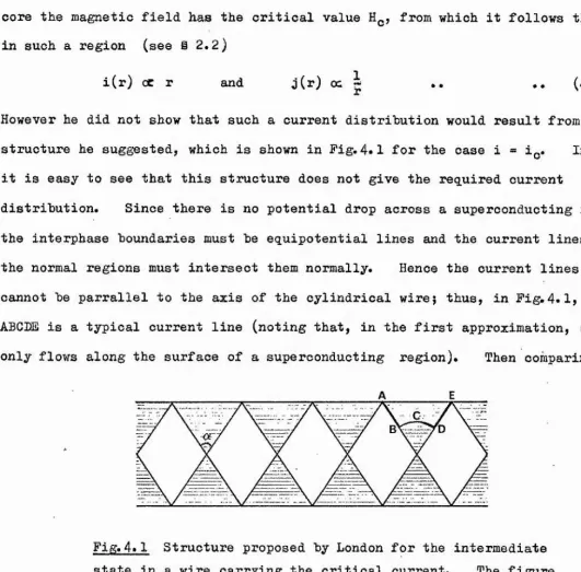
a superconducting core surrounded by a normal sheath is not self-consistent and we are led to assume that the core itself must be in the intermediate state. At equilibrium superconducting-normal interfaces must be electric equipotentials so that if the intermediate state structure is laminar, the laminae must be oriented perpendicularly to the direction of current flow.
These considerations led F. London (1935) to suggest that for i^ < i
the wire would have an intermediate state core of radius r^ < a surrounded by ? a cylindrical sheath in the normal state as shown in Fig. 2.1. The normal i sheath corresponds to the region where the magnetic field is greater than Hg. London assumed that everywhere inside the core the field is Hg, so that the current flowing within any radius r < r^ should be
i(r) = 2«rHg .. .. (2.2)
and, in particular, the total current carried by the intermediate state core
IS i(r^) = 2%rgH
core ' O'
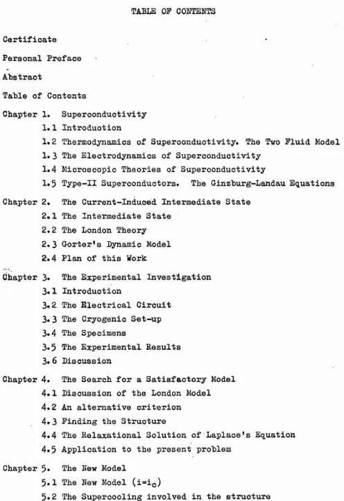
At the surface of the core the normal regions merge continuously into the (2.3)
^ / \ / \
t
/ \ ’
[image:24.613.141.392.555.690.2]2.3T
sheath so that there cannot he any discontinuity in the current density at the core boundary (r = r^)* Within the core the current density is given by
J(r) = (l/2nr). (di/dr) - H^/r .. (2.4) In the normal sheath itself the current density must be uniform so that we can write
^sheath ,= = V ' o •• •• A 5 )
Hence thé total sheath current is:
Lheath ‘ To^)Ag .. (2.6)
Since the sheath is fully normal, its resistance per unit length is
«sheath = EnaV(a^-ro^) •• .. (2.7)
where is the normal resistance per unit length of wire. The electric field per unit length of wire will be
E - Hi = Rdgbeath * Lore^
E - R .. (2.8)
9) or, considering the sheath only,
^sheath* ^sheath *'n"**o'*c It follows that
E - E/i - 1 + |l - (2aaHg/i)^* = + Jl - ( i g / i ) ^ (2.
.0
0.5
e# 0
1.0
i/i.
2.4 % j;
■ i
Fig.2.2 The resistance transition predicted by London (solid line) compared with experimental values obtained by Scott (1948) for 0.286 mm. diameter Indium wire.
shown in Fig.2.2 where Scott's results for a 0.286 mm. diameter Indium wire are compared with the curve of (2.9).
Several attempts have been made to explain the discrepancy between
London's theory and experimental results. Scott (1948) found that the value of the resistance jump p varies approximately inversely with the wire diameter and suggested that London's expression (2.9) might hold for thick wires.
However later work on thick wires by Freud et al (1968) has shown that this
was not the case. Kuper (1952) attributed the discrepancy to additional resistance due to the scattering of conduction electrons at the interphase boundaries. An accurate calculation of this effect is difficult because London's model does not specify the periodicity of the structure. Kuper's approximate calculations showed that boundary scattering would indeed
increase the value of resistance, in particular that of p, but consistent agreement with experimental values was still not obtained.
Troinar (I96O) investigated the variation of p with temperature for tin samples and made some of his measurements at temperatures below the Helium X point. His results indicate that the value of p increases as the
critical current becomes larger. Further, for impure specimens with high
" " I l : ' • C .
2.51!
residual resistivity Troinar observed a discontinuous fall in the value of p '■ as the temperature is lowered below the X point, but he did not find a similar | effect for pure *thick* samples of low residual resistivity* These findings suggest that the value of p depends on and increases with joule heating in the I specimen. Berkovich and Lapir (1963) have given a theoretical treatment in which they have modified London’s treatment to take account of joule heating* They obtain the following modified formula for the resistance of the wires
R = 0 for 0 < i < i,
E . ______ ^ [1 + 6/2 + J 1 + 6
-for < i < ~z { .. (2.10)
J 1+6 JT
ic
R « for — < i
JT
where 5 = (Po/8% ha), is the resistivity of the normal phase and
h is the coefficient for heat transfer across the sample - liquid Helium
boundary. Berkovich and Lapir find that in the case of samples of relatively high residual resistance the values of h required to fit expression (2.10) to the experimental curves of Troinar lie within the range of values obtained from direct measurements of h. However (2.10) does not agree well with J Troinar*s results for samples of high purity. Besides, Troinar*s
observa-tions show that even at temperatures close to T«, where joule heating effects 3
1
should be small, the range of values obtained for p does not agree with the 4
London value of 0.5* Thus joule heating alone cannot account for the |
discrepancy between*s London's expression (2.9) and experimental results.
1
2.3 GORTER'S BYMMIC MODEL: #
Gorter (1957) suggested that the boundaries between normal and super- I conducting regions might tend to orient themselves parallel instead of | perpendicular to the direction of current flow. In the model proposed
2.6
!□
CT":
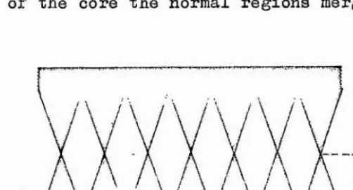
Fig. 2.3 Sorter's dynamic model for the intermediate state structure in a current carrying wire.
normal and superconducting regions as shown in Pig.2.3» Gorter showed that the current through the wire would cause a continuous inward motion of the
shells resulting in eddy current losses. Gorter and Potters (1958) calculated the effective resistance due to the eddy current losses and obtained an
expression identical to the London expression (2.9)* They also showed that if supercooling occurs this leads to an increase in resistance over that given by (2. 9) by only a few percent when the current is slightly greater than i^;
this increase can only account for a fraction of the discrepancy between experimental results and expression (2.9)«
In Gorter' 8 model the surface sheath of the wire would alternate between the normal and superconducting states and it follows that the magnetic field produced by the current on the surface of the wire should have a variable component. Shalnikov (1957) attempted to measure this variable component of the field but failed to observe any periodic or non-periodic signals. In another series of experiments Shalnikov used magnetic powder to display the structure of the intermediate state in a wire and found that the superconduc ting auid normal regions oriented themselves perpendicularly to the general direction of current flow.
fins;
[image:28.612.9.554.17.652.2]" ■.... ^... 'I
I
0.64 < X < 0.707* Thus Gorter*3 model has not proved satisfactory from #
I
either a theoretical or an experimental point of view.
2.4 PIAN OP THIS WORK:
We have seen that neither of the models proposed by London and Gorter â gives quantitative agreement with experimental values on the return of
resistance and that Gorter*s model also appears to be unsatisfactory from a 3
theoretical point of view.
At the start of this work it was decided to check the experimental ; situation by some careful measurements of the return of resistance in Indium ; wires - these measurements are described in the next chapter. A few experi- ! ments were sufficient to confirm the general trend of previous results. The fact that various workers under different experimental conditions had all Æ obtained results which were similar in nature, in qualitative agreement with J London's model but with a considerable quantitative discrepancy, suggested to i us that this discrepancy was perhaps not entirely due to secondary effects.
In Chapter 4 a closer look is taken at the London model, it is shown that the model is theoretically unsatisfactory in some ways and the numerical methods used to obtain a more self-consistent model are described. The new model -itself is presented in Chapter 5 and it is shown that the return of resistance 4; as predicted by this model agrees better with experimental results than is the f case with the models presented earlier in this chapter. The various
secondary effects mentioned in connection- with London's model may also be applied to the present model and taken together they provide a reasonable understanding of experimental results.
During the course of this work another model was proposed by Andreev(l968).
1
This is briefly described in Chapter 6 where it is shown that Andreev's model 1 ’1 does not agree well with experiment and that it is perhaps not quite satis- J factory from a theoretical point of view either. Finally, Chapter 7 concludes
3* THE EXPERIMENTAL INVESTIGATION
3.1 INTRODUCTION;
As mentioned in the previous chapter, the resistance transition in Type-I wires had been experimentally investigated by a number of workers prior to this i work. However in almost all these cases curves showing the return of resistance as a function of current had been obtained by joining discreet experimental
(i,R) points. This did not make for the most accurate determination of the ^ resistance jump f> at the critical current. A prime object of our experimental ■ investigation was to obtain a continuous plot so that the value of p could be more accurately determined.
Basically the experiment consisted of passing a very slowly but steadily increasing current through a superconducting wire which was kept at a constant temperature T just below the critical temperature Tq and of continuously
monitoring the voltage across the wire. The current through the specimen and the voltage across it were plotted on an X - Y recorder which thus plotted a 4 V-I curve for the specimen at that particular temperature. From this it was easy to compute a resistance-current curve for the specimen. Thus for any given specimen a range of R-I curves could be obtained at different temperatures close to but below T^,
3.2 THE ELECTRICAL CIRCUIT;
Fig. 3.1 shows a block diagram of the electrical circuit used. |
P is a remotely programmable constant current power supply. Two Hewlett- Packard models - 6824A and 6284A - were used allowing coverage of 0 - 1.2 Amps. ^ and 0 - 4 . 0 Amps, respectively. These models were chosen for good load | regulation on constant current operation, for their high stability and low noise 3
i
characteristics. The current output was controlled by remote resistance il programming at approximately $00 ohms per ampere. A ten turn ($00 ohm orm
X Y
3.2:1 %
Fig. 3# 1 Block, diagram of the electrical circuit.
was achieved by using a small variable speed d. c. motor m to drive the potentio meter, with an appropriate gear system. The speed of this motor and hence the rate of change of the current i in the main circuit could be controlled by regulating the output voltage of a laboratory power supply p which was used to power the motor m. The rate of change of current could be varied between about | 50mA/mt. and 3A/mt.
The main circuit was composed of the following other elements:
(i) D is an oil-immersed, four terminal standard resistor of nominal value
1 ohm and rated to carry upto 3 Amps, with a quoted accuracy of 0.001^. It I served two purposes:
(a) The value of the current could be determined accurately by measuring theJ voltage across D with a d. c. potentiometer V. This enabled the current to be determined to ± 0.25mA and was used to calibrate the scale of the Beckman f potentiometer in terms of current.
3.3
thus enabling the value of the current to be plotted along the X axis.
(ii) A is an Avometer which, used on its current ranges, provided a rough
indication of the current,
(iii) S represents the specimen of superconducting wire and will be described below. The potential.across S was fed into
(iv) K, a low noise d,c. amplifier with an adjustable gain of upto 10®. The model used was a Keithley 149 milli-microvoltmeter which, on its most sensitive range, gave a full scale deflection for 0.1 microvolt. The accuracy was within
zi» of full scale on all ranges. The input shorted noise level was quoted at less than 3 nanovolts peak to peak and, in practice, was always found to be below 5 nanovolts peak to peak. The Keithley Model 149 acting as an amplifier gave a d. c. output (10 volts for full-scale deflection) and this was fed into the: Y channel of
(v) the X-Y recorder XY. As indicated previously, the potential across the standard 1 ohm resistor was fed into the X channel of this recorder; thus the recorder gave us a continuous plot of V-I for the specimen involved. The voltages fed into the recorder being in the ranges 0 to 3 volts and 0 to 10
volts, the recorder did not require sensitive amplifiers and the model used was a Moseley 7035*
(vi) L is a load resistor. The remaining elements of the main circuit had a total resistance of just over an ohm and the value of L was chosen in such a way that the Power Supplies P were delivering about two thirds of their total f available power under conditions of maximum current^
3.3 THE CRYOGBKIC SET-UP:
Cryogenic experiments are fairly common nowadays and, as our experiment was a simple one and did not require any special techniques, the apparatus used -will be described briefly.
Pig. 3*2 shows a sketch of the experimental set-up used. H is the Helium dewar made from Monax glass which is attached with an *0*ring seal to the
j
3.4
P U M P
Fig. 3» 2 Schematic of the cryogenic set-up.
cryostat neck and sits inside the liquid nitrogen dewar N. The latter is surrounded by a Mumetal cylinder G, open only at the top, whose dimensions are such that the lower part of the helium dewar (upto a height of about 10 cms. from the bottom) is screened from the earth's magnetic field. It was found that the shielding was about effective.
3.5
particularly useful for monitoring changes of pressure. .. Another quarter inch line V connected the cryostat to the helium gas recovery line R. W is a one inch line connecting the cryostat via valve u to a rotary pump whose exhaust' could, when the system was pumping on helium, he connected to the helium gas recovery line R. The big ya.flve u could be bypassed by a quarter inch line containing a sixteen turn needle valve v and this provided a very fine control of the pumping rate. By monitoring the pressure of the system on the oil manometer and/or the mercury manometer with the help of a cathetometer and by using the needle valve v, the pressure could be kept constant to within about ± 0.5 mm on the oil manometer which, in the relevant range of pressure, is equivalent to keeping the temperature constant to within ± 0.25 millidegrees. During the later stages of the work the use of a Cartesian Manostat made it easier to control the temperature in the system.
The cryostat top plate T has an opening F for the liquid helium transfer siphon and several glass-metal seals S for taking electrical leads into the cryostat. These were of the hollow type and copper leads were passed through them and soldered on both sides. Thus the potential leads to the specimen were all copper leads thereby reducing thermal noise. Seals were required for two voltage and two current leads to the specimen, two current leads to a carbon resistor heater h and an earth point. The carbon resistor had a nominal room temperature resistance of 10 ohms and was fed from the power supply p (Pig.3#l)» It was used to raise the temperature of the helium bath if required and also to help boil off excess helium at the end of an experimental run.
Three stainless steel tubes r soldered to the base of the top plate helped support two copper discs b which acted as heat shields. The copper plates had concentric circular holes cut in them.to allow the helium transfer siphon to pass through. At their lower ends the tubes r terminated in hooks from which ' the specimen holder A was suspended by means of nylon thread.
3.6
t
4;
of tufnol, a bakélite, of radius about one inch so that it just slipped comfor tably into the helium dewar and about 2^ inches long. The cylinder had
circumferential ruts cut into it so that the specimen could be laid in one of these ruts, without completing a full circle. In this way it was possible to mount a longer specimen (upto about 6 cms. in length) at the same horizontal level than would be possible with a straight specimen. When specimens were superconducting wires of diameter of the order of 1.0 mm. or .larger, the normal resistance of the specimens were sufficiently
small that the noise (mainly thermal) voltage became significant enough to make the experi ment unsatisfactory. For such wires longer specimens were used and these were wound round the former as shown in Pig. 3* 3 so that
(a) the winding was non-inductive, and
(b) the magnetic fields due to neighbouring portions of the wire were self-cancelling. Such a specimen would be spread over a height
of about 2 to 3 cms. in the helium so that the temperature of the specimen may vary by about a millidegree, and the resistance jump is slightly less sharp than would otherwise be the case. However by comparing results obtained with long and short specimens of a thin wire, it was found that the value of the resistance jump p itself was the same (to within experimental spread) in both cases. Hence for our purposes the slight spread in the transition was not an important factor.
Enamelled copper wires were used for the current and voltage leads and optimum guages were calculated following Rose-Innes(l959) to minimize the heat input due to thermal conductivity and joule heating. The leads were soldered on to the specimen with Woods Metal solder using a low temperature soldering iron. A 5 Kohra, 25 watts potentiometer was connected in series with the
soldering iron to regulate its temperature.
Pig. 3. 3 Diagram indicating
\
\ \
\
Q
9
«
n
i
?
+» oOQ (6 +»
i
•Hs »<D +> %
»
<D
3
2
PLATE III. Rear view of experimental set-up with the dewars removed and the specimen holder in place#
3.7-An overall view of the experimental set-up is shown in Plate 2 and in I
Plate 3 the specimen holder is shown in situ with the dewar removed.
3.4 THE SPECIMSNSj
The experimental investigation was carried out mainly on Indium specimens* 4 f We were primarily interested in obtaining a few accurate observations ^
(particularly on the resistance jump ) for very pure metal. On the basis
of theory and previous work there was no reason to suppose that the transition % differed fundamentally as between different metals. On several counts it was | particularly convenient to work with Indium:
(a) it is easy to obtain very pure Indium.
(b) with a K value of about 0.11 Indium is a strongly Type-I superconductor. (c) it is relatively easy to extrude Indium wires*
(d) Indium anneals at room temperature.
(e) Indium has a critical temperature of 3 * 4 0 ? which is very convenient for experimental purposes*
Pure Indium was obtained from two sources: Johnson Matthey and Co., London, |
iî
whose Indium had a quoted purity of
99
*
9995
^ »
and Consolidated Mining Co.j
(Cominco) of Montreal, Canada, who quoted the purity of their Indium at99
*
9999
! ^ * i
Resistance measurements on the Indium specimens at room temperature and at 4.2®K^ showed the Cominco Indium to be much the purer and most of the experiments were done with their Indium. It was interesting to note that the purer Indium was much stickier too. This stiokiness constitutes the main problem in extruding j Indium wires, as the Indium tends to creep up the sides of the extruder piston < and jam it. With this in view, an extruder was made out of tool steel with the -piston made to fit the cylinder to a fine degree of tolerance and the whole was heat treated in an atmosphere of hydrogen. The piston head was recessed and | this helped to reduce the creep of Indium up the cylinder wall during extrusion. The extrusions were carried out at room temperature with the help of an automatic... - ■ ... 3.8 'S 4 I
within ± 0.005 mm.
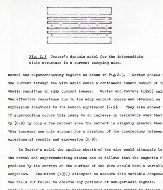
Altogether seven Indium specimens were used with their diameters varying in the range 0,25 mm. to 1.65 mm. Additionally experiments were carried out with
one specimen of Tin wire of 0.5 mm. diameter and a specimen of Thallium wire of #
s
1.0 mm. diameter. Both of these wires were obtained from Metals Research Ltd., I Roys ton. Table 3.1 describes the specimen used; the purity given in column 4 is that quoted by the suppliers while column 5 gives the ratio ^4,3 / ^ 9 3 of the resistivities of the specimens at the temperature of liquid helium at atmospherics pressure and at room temperature.
fv
fv
In the case of Indium I the current and r ... ..— voltage leads were connected close together
near the ends of the specimen as indicated in
Fig.3"4(a). However this set-up resulted in r 4V — ^ - ■ ■ ■ ' J a tail in the resistance transition curve, i.e. Jj
instead of a sharp jump in resistance when the
(a)
(b)
current became critical, the resistance showed Fig.3.4 Sketch showing the a slow increase even before iç was reached as relative positions where the
voltage and current leads were attached to the specimen
of Indium II the voltage leads were connected (a) for Indium I and Thallium may be seen in Figs.3* 5 and 3* 8. In the case
I and (b) for all other specimens.
to the specimen at points about a cm. away from where the current leads were soldered, as
shown in Fig. 3#4(b) and no 'tail' was obtained (see Figs. 3* 6 and 3*9). This
3-9 I I CM AO •H +*a bO ♦H *d
+»03 •p©
O o > P A cy •H r4 (d +» a ©a •riU
©A A© M -P
© a
© ©
fH .4+» •HA
rn « g m © 9 E4 © ©a •H O©
P i ©
xa ON © PO -p CO 4-1O 0o •H
«PP i •HA Ü © © A
I
a (D•H 8
o (3
a> a Pi w To CM 0 \ <7\ urs Zq
I
+>I
§ 03 M To CM t— o\ CTv urv d I y roiH To to to
I
M M M M iH
ir\
iH
« « S:Cr\ CT\ (T \ cr\ CTN cA CT\ §
I
O Os ITNIT\
M M rO VO VO iH CT\ ON ON cfv ON CTN ON ON ON ON ON OV (A ON %(T\ g;
ITN gi o
1 1 1 1
o o o o
TdT 1 -o *p1 1
* H
M H >
H H H
m
a ap ) to A 5
M M H H
A A A A
Ï25 Î25 523 A
M H H H
I
I
H
I
t t s s
H N
o oj
UN. •
m M
%ON
» ON
ON ON ON
O <D 8 8 %
I
0> fHI
ON C7N 1 © to P P Ao > ©o UN Ap
fH O >* P © A P P » î>» •P fH -P P A O A H O
ua 1 ato
© o H
© 'p A 'vt'
© 1 523
H ro
© a A
fH o A
© A P
•P A
© bO
a *P© P
A A P © A 44 44 P •rH •H *P *P H ©
H H P
•H
g; P
A to iH
H M A
A H A M
A IZf ©
Î23 H
H ©
E4 E4 * P
3.10
connected as shown in Pig.3.4(h) with a minimum gap of 1.0 cm. between the current and voltage connections.
3.5 THE EXPERIMENTAL RESULTS:
The output from any experiment consisted of an X-Y recorder plot of the current-voltage characteristic for a specimen kept at a constant temperature. Three typical curves are shown in Pigs. 3*5» 3*6 and 3*7, and it can be seen from these continuous plots (except in Pig. 3*5 for reasons discussed in the previous paragraph) that when the current reaches its critical value the resistance jump is well defined. We thus obtain a more accurate value of j> than would be
possible if discrete measurements of (V,i) were made and a curve drawn to pass through them. Pigs. 3*6 and 3*7 show that the resistance jump at i = iç» is spread over a small current range; this is an experimental artefact due to the small but finite rate of change of current. By manually operating a very fine -current control it was possible to eliminate the transition width and it was found that the values of p obtained in this way lie within the experimental .
spread in the values of j> obtained from the continuous plots. I
I
It is the resistance of a wire specimen rather than the voltage across it ;ij that is the basic quantity of interest to us. Accordingly our experimental | results are presented in Pigs. 3».8 to 3*15 in the form of curves showing the | I variation of the resistance ratio R/Rn with current i. These have been obtained]i by conversion from the V-i curves on a point by point basis and since the latter ! i were continuous curves, it has been possible to use a large number of points at |
regions of large curvature. ' ]
■I
The inherent noise level in the experiments was of the order of 20 nano- volts. As may be seen in Pigs. 3*5 to 3.7, there were occasional random excursions of the order of 100 nanovolts or less - if these occurred where the curvature was small, the curve was smoothed out, but when they happened near the sharp transition, the curve was rejected and the experiment was repeated if |
3.11
H t ,__L:
M
M
rH
3.12
I
M
•H
3.13
«H
M
u
•H
S
4a
ro %
•H CQ
S
A +3 m ü +*ra
•H CQ
S
' % T. Ah.,
3.14
T
CL ^ 3 , k
b: 3.
c: 3.
3
: 3
i (amps.)
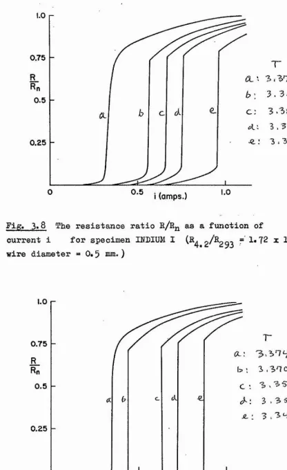
Fig. 3.8 The resistance ratio R/R^ as a function of
current i for specimen INDIUM I (R^ 2^^^293 ^ z 10
wire diameter » 0»5 mm.)
1.0
0.75
3
0.5
0.25
i (amps.)
0 1.0
Fig. 3.9 The resistance ratio R/R^ as a function of
[image:46.612.80.496.18.698.2]. v - .y
3.15
1.0
0.75
CLl R_
Rn
0.5
0.25
0 0.5 I (amps.) 1.0
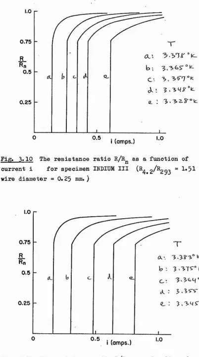
Fig. 3«10 The resistance ratio R/R^ as a function of
current i for specimen INDIUM III (R^ 2^^293 ~ 1*51 % 10”^, wire diameter = 0.25 mm. )
1.0
0.75
0.5
0.25
0 0.5 i (amps.) 1.0
Fig, 3«11 The resistance ratio R/R^ as a function of
[image:47.612.85.488.15.736.2] [image:47.612.112.465.19.293.2]0.75
T
0.5
0.25
1.0
i (amps.) 0
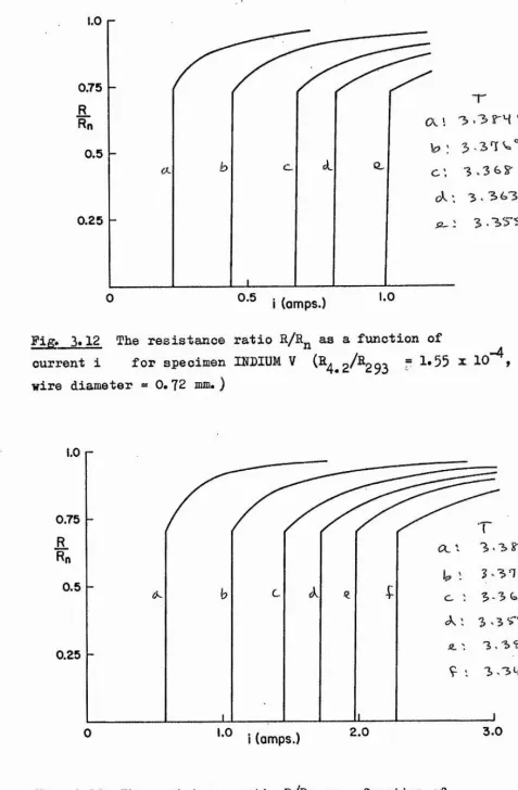
Figé 3.12 The resistance ratio R/R^ as a function of
current i for specimen IRDIUM V (^4,2^^293 ^ 1*55 % 10"^> wire diameter ~ 0#72 mm. )
0.75
(LI 3'3^2-K.
0.5
9 I 3.34&")c
0.25
3.0 2.0
i (omps.) 0
%
'fît
Fig. 3.13 The resistance ratio R/R^ as a function of
[image:48.619.64.542.26.755.2]3 . 1 #
1,0r
0.75
% 0.5
0.25
K h (L
1.0 i (amps.)
b 1 3,31*7 "k C : 3
3 .3G.X ^ ' 3
4: 3 .
4.0
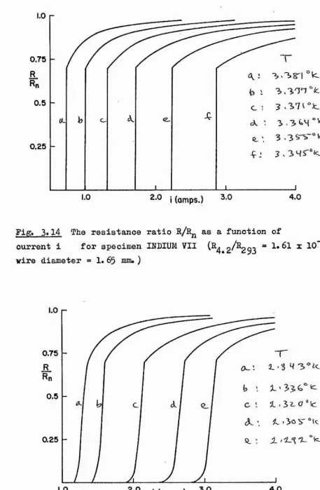
Fig. 3#14 The resistance ratio R/R^ as a function of
current i for specimen IRDIÜM VII (R^ 2^^293 * ^ 10”^, wire diameter * !• 65 mm*)
1.0
0.75 R_
Rn
0.5
0.25
4.0
i (amps.)
1.0
Fig» 3*15 The resistance ratio R/R^ as a function of
[image:49.612.67.524.13.712.2] [image:49.612.99.489.20.289.2]3* Ip.
3.6 DISCUSSIONS^ ?
We shall now discuss the conclusions that may be drawn from our experimen-i
tal results.
With certain exceptions which will be discussed below, the basic current- I
induced trainsition in superconducting wires may be described as follows: for
values of current less than a certain critical value i^ the wire is fully i
superconducting; at the critical current resistance suddenly appears and jumps s
to a considerable fraction p of the fully normal resistance; as the current f
is increased further, the resistance increases gradually until it asymptotically# reaches the fully normal resistance at a current of about 4ig for very pure
metals. J
For very low current transitions, the resistance jump at ig is not sharply ; defined but becomes smoothed out as may be seen in Figs. 3* 8, 3*9, 3*10 and 3* H
This has been observed before (D. C. Baird, private communication) but is not |
yet properly Understood. However it may be pointed out that a comparision
between the results for INDIUM II and INDIUM IV shows that the effect of making a specimen impure is to increase the range of current over which the resistance %
jump is not sharply defined. Ï
Leaving aside these * low-current * transitions, our results (as well as the
results of other workers) indicate that the value of p varies from 0. 69 -I
upwards. The exact value seems to depend on temperature (i.e. the critical
current), the diameter of the wire and on the purity. For example, Fig.3*16 |
shows the variation of the resistance jump p with critical current for two |
cases: INDIUM II and INDIUM IV. In the case of INDIUM II the value of f goes
up as the critical current increases. However in the case of INDIUM IV, which
is a purer specimen, the value of p remains constant (within the limits of
experimental accuracy) for values of i^ less than about 0. 9 Amps, and then |
begins to increase as the critical current is increased further. In the case i
3.19
0,8
P
0.7
0.6
A INDIUM II
■ INDIUM IV
0.2 0.6 1.0
io (Amps. )
Fig.3*16 Variation of the resistance Jump (at i « i^) with critical current for INDIUM II and INDIUM IV specimens.
the value of p remains constant upto at least 1q « 2.5 Amps, (see Fig. 3*1^)# These observations suggest that the value of p is independent of the critical current as long as the latter is below a certain limiting value; this limiting Î
-I
value becomes smaller as the wire becomes thinner or less pure. When the | critical current is greater then the limiting value i]^, p increases as iq
goes up and the increase is larger for less pure specimens.
Fig.3'17 shows the variation of the.resistance jump p with diameter of
wire for very pure Indium where the point corresponding to a wire diameter of 3 mm. has been taken from the work of Freud et al (1968). It appears that p has a value of about 0.695 for thick, pure Indium wires but rises gradually as the wire diameter is reduced below about 1.5 mm, Scott (1948) and Meissner and Zdanis (1958) amongst others had previously studied the variation of as a function of wire diameter. The present work along with that of Freud and his collaborators confirms that even for thick, pure wires the value of
0.75
P
0.7
0.65
3.2g
• This work
• Freud et al (1968)
1 2
Wire diameter (mm.)
Fig. 3»17 Variation of the resistance jump diameter of wire for very pure Indium.
with
is well ahove the figure of 0.5 predicted hy London.
A comparision "between the resistance transitions for relatively impure Indium wire (specimens I and II) and pure Indium wire of about the same diametei; (specimen IV) shows that the less pure specimen reaches its fully normal
resistance fol* a lower value of current than the very pure specimen.
Finally we note that for any given wire, if we restrict ourselves to that
range of current where is independent of iq, all resistance transitions lie
-.1
(within the limits of experimental error) on one basic curve when the normalised resistance
R / R
j i is considered as a function of the reduced currenti / i o *
i
This has been illustrated in Table 3.2 for the case of INDIUM VII. ^
A valid model of the intermediate state in current carrying wires must be able to predict a return of resistance in agreement with the basic experimental;]
I
curve and must also be able to explain the various effects due to temperature, jj
I
purity and diameter of wire which have been detailed above. In Fig.3*18 ‘ j
experimental points taken from the basic resistance transition curves for |
INDIUM III and INDIUM VII are compared with the curve predicted by London.
INDIUM VII is a pure Indium wire of diameter 1. 65 mm. and our previous i
[image:52.614.44.532.18.345.2]