Exploiting Submodular Value Functions for Faster Dynamic Sensor Selection
Yash Satsangi
and
Shimon Whiteson
Informatics Institute, University of AmsterdamAmsterdam, The Netherlands
{y.satsangi,s.a.whiteson}@uva.nl
Frans A. Oliehoek
Informatics Institute, University of Amsterdam Dept. of CS, University of Liverpool [email protected]
Abstract
A key challenge in the design of multi-sensor systems is the efficient allocation of scarce resources such as bandwidth, CPU cycles, and energy, leading to thedynamic sensor se-lectionproblem in which a subset of the available sensors must be selected at each timestep. While partially observ-able Markov decision processes(POMDPs) provide a natural decision-theoretic model for this problem, the computational cost of POMDP planning grows exponentially in the num-ber of sensors, making it feasible only for small problems. We propose a new POMDP planning method that usesgreedy maximizationto greatly improve scalability in the number of sensors. We show that, under certain conditions, the value function of a dynamic sensor selection POMDP is submod-ularand use this result to bound the error introduced by per-forming greedy maximization. Experimental results on a real-world dataset from a multi-camera tracking system in a shop-ping mall show it achieves similar performance to existing methods but incurs only a fraction of the computational cost, leading to much better scalability in the number of cameras.
Introduction
Multi-sensor systems are becoming increasingly prevalent in a wide range of settings. For example, multi-camera sys-tems are now routinely used for security, surveillance, and tracking. A key challenge in the design of such systems is the efficient allocation of scarce resources such as the band-width required to communicate the collected data to a cen-tral server, the CPU cycles required to process that data, and the energy costs of the entire system. This gives rise to the dynamic sensor selectionproblem (Spaan and Lima 2009; Kreucher, Kastella, and Hero 2005; Williams, Fisher, and Willsky 2007): selecting, based on the system’s current un-certainty about its environment,K of theN available sen-sors to use at each timestep, whereKis the maximum num-ber of sensors allowed given the resource constraints.
When the state of the environment is static, amyopic ap-proach that always selects the sensors that maximize the im-mediate expected reduction in uncertainty is typically suffi-cient. However, when that state changes over time, a non-myopic approach that reasons about the long-term effects of the sensor selection performed at each step can perform
Copyright c2015, Association for the Advancement of Artificial Intelligence (www.aaai.org). All rights reserved.
better. A natural decision-theoretic model for such an ap-proach is the partially observable Markov decision pro-cess(POMDP) (Astr¨om 1965; Smallwood and Sondik 1973; Kaelbling, Littman, and Cassandra 1998) in which actions specify different subsets of sensors.
In a typical POMDP, reducing uncertainty about the state is only a means to an end. For example, in a robot control task, the robot aims to determine its current location so it can more easily reach its goal. However, dynamic sensor se-lection is a type ofactive perceptionproblem (Spaan 2008; Spaan and Lima 2009), which can be seen as a subclass of POMDPs in which reducing uncertainty is an end in itself. For example, a surveillance system’s goal is typically just to ascertatin the state of its environment, not use that knowl-edge to achieve another goal. While perception is arguably always performed to aid decision-making, in an active per-ception problem that decision is made by another agent, e.g., a human, not modeled by the POMDP.
Although POMDPs are computationally expensive to solve, approximate methods such as point-based planners (Pineau, Gordon, and Thrun 2006; Araya et al. 2010) have made it practical to solve POMDPs with large state spaces. However, dynamic sensor selection poses a different chal-lenge: as the number of sensors N grows, the size of the action space NKgrows exponentially. Consequently, as the number of sensors grows, solving the POMDP even approx-imately quickly becomes infeasible with existing methods.
In this paper, we propose a new point-based planning method for dynamic sensor selection that scales much better with the number of sensors. The main idea is to replace max-imization with greedy maximization (Nemhauser, Wolsey, and Fisher 1978; Golovin and Krause 2011; Krause and Golovin 2014) in which a subset of sensors is constructed by iteratively adding the sensor that gives the largest marginal increase in value. Doing so avoids iterating over the entire action space, yielding enormous computational savings.
approximation thereof. To our knowledge, these are the first results demonstrating the submodularity of value functions and bounding the error of greedy maximization in the full POMDP setting.
Finally, we apply our method to a real-life dataset from a multi-camera tracking system with thirteen cameras in-stalled in a shopping mall. Our empirical results demonstrate that our approach outperforms a myopic baseline and nearly matches the performance of existing point-based methods while incurring only a fraction of the computational cost.
Background
In this section, we provide background on POMDPs, dy-namic sensor selection POMDPs, and point-based methods.
POMDPs
A POMDP is a tuple hS, A,Ω, T, O, R, b0, γ, hi. At each
timestep, the environment is in a state s ∈ S, the agent takes an action a ∈ A and receives a reward whose ex-pected value is R(s, a), and the system transitions to a new state s0 ∈ S according to the transition function T(s, a, s0) = P r(s0|s, a). Then, the agent receives an ob-servation z ∈ Ω according to the observation function O(s0, a, z) = P r(z|s0, a). The agent can maintain a belief b(s) using Bayes rule. Givenb(s)andR(s, a), the belief-basedreward,ρ(b, a)is:
ρ(b, a) =X s
b(s)R(s, a). (1)
A policyπspecifies how the agent will act for each belief. The valueVtπ(b)ofπgiventsteps to go until the horizonh is given by theBellman equation:
Vtπ(b) =ρ(b, aπ) +γ
X
z∈Ω
P r(z|aπ, b)Vtπ−1(b
z,aπ).
(2)
The action-value functionQπ
t(b, a)is the value of taking ac-tionaand followingπthereafter:
Qπt(b, a) =ρ(b, a) +γX z∈Ω
P r(z|a, b)Vtπ−1(bz,a). (3)
The optimal value functionVt∗(b)is given by theBellman optimality equation:
Vt∗(b) = max a Q
∗
t(b, a)
= max
a [ρ(b, a) +γ
X
z∈Ω
P r(z|a, b)Vt∗−1(bz,a)]. (4)
We can also define theBellman optimality operatorB∗: (B∗Vt−1)(b) = max
a [ρ(b, a) +γ
X
z∈Ω
P r(z|a, b)Vt−1(bz,a)],
(5) and write (4) as:Vt∗(b) = (B∗Vt∗−1)(b).
An important consequence of (1) is that Vt∗ is piece-wise linear and convex (PWLC). This property, which is exploited by most POMDP planners, allowsVt∗ to be rep-resented by a set of vectors:Γt = {α1, α2. . . αm}, where eachα-vector is an|S|-dimensional hyperplane representing Vt∗(b)in a bounded region of belief space. The value func-tion can then be written asVt∗(b) = maxαi
P
sb(s)αi(s).
Dynamic Sensor Selection POMDPs
We model the dynamic sensor selection problem as a POMDP in which the agent must choose a subset of avail-able sensors at each timestep. We assume that all selected sensors must be chosen simultaneously, i.e., it is not possi-ble within a timestep to condition the choice of one sensor on the observation generated by another sensor. This cor-responds to the common setting in which generating each sensor’s observation is time consuming, e.g., because it re-quires applying expensive computer vision algorithms, and thus all observations must be generated in parallel. Formally, a dynamic sensor selection POMDP has the following com-ponents:
• Actions a = ha1. . . aNi are modeled as vectors of N binaryaction features, each of which specifies whether a given sensor is selected or not (assumingNsensors). For eacha, we also define its set equivalenta={i:ai = 1}, i.e., the set of indices of the selected sensors. Due to the resource constraints, the set of all actionsA={a:|a| ≤
K}contains only sensor subsets of sizeKor less.A+= {1, . . . , N}indicates the set of all sensors.
• Observations z = hz1. . . zNiare modeled as vectors of N observation features, each of which specifies the sen-sor reading obtained by the given sensen-sor. If sensen-sor i is not selected, then zi = ∅. The set equivalent of z is z = {zi : zi 6= ∅}. To prevent ambiguity about which sensor generated which observation inz, we assume that, for alliandj, the domains ofziandzjshare only∅.
• The transition functionT(s0, s) = P r(s0|s)is indepen-dent ofabecause the agent’s role is purely observational.
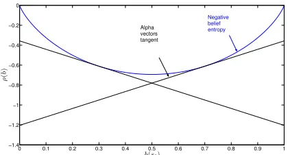
• The belief-based reward ρ(b) is also independent of a and is typically some measure of the agent’s uncertainty. A natural choice is the negative entropy of the belief: ρ(b) =−Hb(s) =Psp(s) log(p(s)). However, this def-inition destroys the PWLC property. Instead, we approxi-mate−Hb(s)using a set of vectorsΓρ={αρ
1, . . . , αρm}, each of which is a tangent to −Hb(s), as suggested by (Araya et al. 2010). Figure 1 shows the tangents for an example Γρ for a two-state POMDP. Because these tan-gents provide a PWLC approximation to belief entropy, the value function is also PWLC and can thus be com-puted using standard solvers.
Point-Based Value Iteration
Exact POMDP planners (Smallwood and Sondik 1973; Monahan 1982; Lovejoy 1991; Kaelbling, Littman, and Cas-sandra 1998) compute the optimal Γt-sets for all possible belief points. However, this approach is intractable for all but small POMDPs. By contrast,point-based value iteration (PBVI) (Pineau, Gordon, and Thrun 2006) achieves much better scalability by computing theΓt-sets only for a set of sampled beliefsB, yielding an approximation ofVt∗.
At each iteration, PBVI computesΓt givenΓt−1 as
fol-lows. The first step is to generate intermediateΓzt,a-sets for alla∈Aandz∈Ω:Γtz,a={αz,a:α∈Γ
t−1},where
αz,a(s) =γX s0∈S
0 0.1 0.2 0.3 0.4 0.5 0.6 0.7 0.8 0.9 1 −1.4
−1.2 −1 −0.8 −0.6 −0.4 −0.2 0
b(s1)
ρ
(
b
)
Negative belief entropy
[image:3.612.65.275.60.173.2]Alpha vectors tangent
Figure 1: Tangents approximating negative belief entropy.
The next step is to use the intermediate sets to generate sets Γa
t ={αa,b:b∈B}, where
αa,b= arg max αρ∈Γρ
X
s
b(s)αρ(s)+X
z
arg max αz,a∈Γz,a
t
X
s
αz,a(s)b(s).
The final step is to find the best vector for eachb ∈ Band generateΓt. To facilitate explication of our algorithm in the following section, we describe this final step somewhat dif-ferently than Pineau, Gordon, and Thrun (2006). For each b∈Banda∈Awe must find the bestαa,b∈Γat:
α∗a,b= arg max αa,b∈Γat
X
s
αa,b(s)b(s), (6)
and simultaneously record its value: Q(b,a) =
P
sα
∗
a,b(s)b(s). Then, for each b ∈ B, we find the best vector across all actions:αb=α∗a∗,b, where
a∗= arg max
a∈A
Q(b,a). (7)
Finally,Γtis the union of these vectors:Γt=∪b∈Bαb.
Greedy PBVI
The computational complexity of one iteration of PBVI is O(|S||A||Γt−1||Ω||B|)(Pineau, Gordon, and Thrun 2006).
While this is only linear in |A|, in our setting|A| = NK
. Thus, PBVI’s complexity isO(|S| NK
|Γt−1||Ω||B|),
lead-ing to poor scalability in N, the number of sensors. In this section, we propose greedy PBVI, a new point-based POMDP planner for dynamic sensor selection whose com-plexity is only O(|S||N||K||Γt−1||Ω||B|), enabling much
better scalability inN.
The main idea is to exploit greedy maximization (Nemhauser, Wolsey, and Fisher 1978), an algorithm that operates on a set functionF : 2X→
R. Algorithm 1 shows
the argmax variant, which constructs a subsetY ⊆Xof size Kby iteratively adding elements ofX toY. At each itera-tion, it adds the element that maximally increasesF(Y).
To exploit greedy maximization in PBVI, we need to re-place an argmax overAwithgreedy-argmax. Our alterna-tive description of PBVI above makes this straightforward: (7) contains such an argmax, andQ(b,·)has been intention-ally formulated to be a set function overA+. Thus, imple-menting greedy PBVI requires only replacing (7) with:
a∗=greedy-argmax(Q(b,·), A+, K). (8)
Algorithm 1greedy-argmax(F, X, K)
Y ← ∅
form= 1to Kdo
Y ←Y ∪ {arg maxe∈X\Y F(Y ∪e)}
end for
returnY
Note that, since the point of greedy maximization is not to iterate overA, it is crucial that our implementation does not first computeα∗a,bandQ(b,a)for alla ∈A, as this would already introduce an|A| = NKterm into the complexity. Instead,α∗a,bandQ(b,a)are computed on the fly only for the a’s considered bygreedy-argmax. Since the complexity of
greedy-argmaxis onlyO(|N||K|), this yields a complexity
for greedy PBVI of only O(|S||N||K||Γt−1||Ω||B|). Note
also that theαz,athat are generated can be cached because they are not specific to a givenband can thus be reused.
Using point-based methods as a starting point is essential to our approach. Exact methods, because they computeV∗ for all beliefs, rely on pruning operators instead of argmax. Thus, it is precisely because PBVI operates on a finite set of beliefs that argmax is performed, opening the door to using
greedy-argmaxinstead.
Analysis: Bounds given Submodularity
In this section, we present our core theoretical result, which shows that, under certain conditions, the most important of which issubmodularity, the error in the value function com-puted by backups based on greedy maximization is bounded. Later sections discuss when reward based on negative belief entropy or an approximation thereof meets those conditions. Submodularity is a property of set functions that corre-sponds to diminishing returns, i.e., adding an element to a set increases the value of the set function by a smaller or equal amount than adding that same element to a subset. In our notation, this is formalized as follows. The set function Qπt(b,a)is submodular ina, if for everyaM ⊆aN ⊆A+ andae∈A+\aN,
∆Qb(ae|aM)≥∆Qb(ae|aN), (9)
where∆Qb(ae|a) =Q π
t(b,a∪ {ae})−Qπt(b,a)is the dis-crete derivativeofQπ
t(b,a). Equivalently,Qπt(b,a)is sub-modular if for everyaM,aN ⊆A+,
Qπt(b,aM∩aN)+Qπt(b,aM∪aN)≤Qπt(b,aM)+Qπt(b,aN). (10) Submodularity is an important property because of the following result by Nemhauser, Wolsey, and Fisher (1978):
Theorem 1. IfQπt(b,a)is non-negative, monotone and sub-modular ina, then for allb,
Qπt(b,aG)≥(1−e−1)Qπt(b,a∗), (11)
whereaG =
greedy-argmax(Qπ
t(b,·), A+, K)and a∗ = arg maxa∈AQπ
t(b,a).
backup, as greedy PBVI does. In this section, we establish such a bound. Let thegreedy Bellman operatorBGbe:
(BGVt−1)(b) =
G max
a [ρ(b,a) +γ X
z∈Ω
P r(z|a, b)Vt−1(bz,a)],
wheremaxG
a refers to greedy maximization. This
immedi-ately implies the following corollary to Theorem 1:
Corollary 1. Given any policy π, if Qπt(b,a) is non-negative, monotone, and submodular ina, then for allb,
(BGVtπ−1)(b)≥(1−e−1)(B∗Vtπ−1)(b). (12)
Proof. From Theorem 1 since(BGVπ
t−1)(b) = Qπt(b,aG) and(B∗Vπ
t−1)(b) =Qπt(b,a∗).
In addition, we can prove that the error in the value func-tion remains bounded after applicafunc-tion ofBG.
Lemma 1. If for allb,ρ(b)≥0,
Vtπ(b)≥(1−)Vt∗(b), (13)
andQπ
t(b,a)is non-negative, monotone, and submodular in a, then, for∈[0,1],
(BGVtπ)(b)≥(1−e−1)(1−)(BGVt∗)(b). (14)
Proof. Starting from (13) and, for a givena, on both sides addingγ≥0, taking the expectation overz, and addingρ(b) (sinceρ(b)≥0and≤1):
ρ(b)+γEz|b,a[Vtπ(b
z,a)]≥(1−)(ρ(b)+γ
Ez|b,a[Vt∗(b
z,a)]).
From the definition ofQπ
t (3), we thus have:
Qπt+1(b,a)≥(1−)Q∗t+1(b,a) ∀a. (15)
From Theorem 1, we know
Qπt+1(b,aGπ)≥(1−e−1)Qπt+1(b,a∗π), (16)
whereaGπ =greedy-argmax(Qπt+1(b,·), A+, K)anda∗π= arg maxaQπ
t+1(b,a). Since Qπt+1(b,a∗π) ≥ Qπt+1(b,a)for
anya,
Qπt+1(b,aGπ)≥(1−e−1)Qπt+1(b,aG∗), (17)
where aG∗ = greedy-argmax(Q∗t(b,·), A+, K). Finally, (15) implies thatQπ
t+1(b,aG∗)≥(1−)Q∗t+1(b,aG∗), so:
Qπt+1(b,aGπ)≥(1−e−1)(1−)Q∗t+1(b,aG∗) (BGVtπ)(b)≥(1−e−1)(1−)(BGVt∗)(b).
Next, we define thegreedy Bellman equation:VG t (b) = (BGVG
t−1)(b), where V0G = ρ(b). Note that VtG is the true value function obtained by greedy maximization, with-out any point-based approximations. Using Corollary 1 and Lemma 1, we can bound the error ofVGwith respect toV∗.
Theorem 2. If for all policiesπ,Qπ
t(b,a)is non-negative, monotone and submodular ina, then for allb,
VtG(b)≥(1−e−1)2tVt∗(b). (18)
Proof. By induction ont. The base case,t = 0, holds be-causeVG
0 (b) =ρ(b) =V0∗(b).
In the inductive step, for allb, we assume that
VtG−1(b)≥(1−e−1)2t−2Vt∗−1(b), (19) and must show that
VtG(b)≥(1−e−1)2tVt∗(b). (20) Applying Lemma 1 withVπ
t = VtG−1 and(1−) = (1−
e−1)2t−2to (19):
(BGVtG−1)(b)≥(1−e−1)2t−2(1−e−1)(BGVt∗−1)(b) VtG(b)≥(1−e−1)2t−1(BGVt∗−1)(b).
Now applying Corollary 1 withVtπ−1=Vt∗−1:
VtG(b)≥(1−e−1)2t−1(1−e−1)(B∗Vt∗−1)(b) VtG(b)≥(1−e−1)2tVt∗(b).
Analysis: Submodularity under Belief Entropy
In this section, we show that, if the belief-based reward is negative entropy, i.e., ρ(b) = −Hb(s), then under certain conditionsQπt(b,a)is submodular, non-negative and mono-tone, as required by Theorem 2. We start by observing that: Qπt(b,a) =ρ(b)+
Pt−1
k=1G
π
k(bt,at), whereGπk(bt,at)is the expected immediate reward withksteps to go, conditioned on the belief and action withtsteps to go and assuming pol-icyπis followed after timestept:
Gπk(bt,at) =γ(h−k)X
zt:k
P r(zt:k|bt,at, π)(−Hbk(sk)).
wherezt:kis a vector of observations received in the interval fromtsteps to go toksteps to go,btis the belief attsteps to go,atis the action taken att steps to go, andρ(bk) =
−Hbk(sk), whereskis the state atksteps to go.
Proving that Qπ
t(b,a)is submodular in a requires three steps. First, we show thatGπk(bt,at)equals theconditional entropyofbkoverskgivenzt:k. Second, we show that, under certain conditions, conditional entropy is a submodular set function. Third, we combine these two results to show that Qπ
t(b,a)is submodular. Proofs of all following lemmas can be found in the extended version (Satsangi, Whiteson, and Oliehoek 2014).
The conditional entropy(Cover and Thomas 1991) of a distributionb over sgiven some observations z is defined as:Hb(s|z) =−P
s
P
zP r(s,z) log(b(s|z)). Thus,
condi-tional entropy is the expected entropy givenzhas been ob-served but marginalizing across the values it can take on.
Lemma 2. Ifρ(b) =−Hb(s), then the expected reward at each time step equals the negative discounted conditional entropy ofbkoverskgivenzt:k:
Gπk(bt,at) =−γ(h−k)(Hbk(sk|zt:k))∀π. (21)
Next, we identify the conditions under whichGπ k(b
t,at)
is submodular inat. We use the set equivalentzofzsince submodularity is a property of set functions. Thus:
where zt:k is a set of observation features observed be-tweentandk timesteps to go. The key condition required for submodularity ofGπ
k(b
t,at)isconditional independence
(Krause and Guestrin 2007).
Definition 1. The observation setz is conditionally inde-pendent givensif any pair of observation features are con-ditionally independent given the state, i.e.,
P r(zi, zj|s) =P r(zi|s)P r(zj|s), ∀zi, zj∈z. (23)
Lemma 3. If z is conditionally independent givens then
−H(s|z)is submodular inz, i.e., for any two observations zM andzN,
H(s|zM ∪zN) +H(s|zM∩zN)≥H(s|zM) +H(s|zN). (24)
Lemma 4. Ifzt:kis conditionally independent givenskand ρ(b) =−Hb(s), thenGkπ(bt,at)is submodular inat∀π.
Now we can establish the submodularity ofQπ t.
Theorem 3. If zt:k is conditionally independent given sk and ρ(b) = −H
b(s), then Qπt(b,a) = ρ(b) +
Pt−1
k=1G
π k(b
t,at)is submodular ina, for allπ.
Proof. ρ(b)is trivially submodular ina because it is inde-pendent ofa. Furthermore, Lemma 4 shows thatGπ
k(b t,at)
is submodular inat. Since a positively weighted sum of sub-modular functions is also subsub-modular (Krause and Golovin 2014), this implies thatPt−1
k=1G
π k(b
t,at)and thusQπ t(b,a) are also submodular ina.
While Theorem 3 shows that QG
t(b,a) is submodular, Theorem 2 also requires that it be monotone, which we now establish.
Lemma 5. IfVπ
t is convex over the belief space for allt, thenQπ
t(b,a)is monotone ina, i.e., for allbandaM ⊆aN, Qπt(b,aM)≤Qπt(b,aN).
Lemma 5 requires thatVπ
t be convex in belief space. To establish this forVtG, we must first show thatBGpreserves the convexity of the value function:
Lemma 6. IfρandVtπ−1are convex over the belief simplex, thenBGVπ
t−1is also convex.
Tying together our results so far:
Theorem 4. If zt:k is conditionally independent givensk andρ(b) =−Hb(s), then for allb,
VtG(b)≥(1−e−1)2tVt∗(b). (25)
Proof. Follows from Theorem 2, given QG
t(b,a) is non-negative, monotone and submodular. Forρ(b) =−Hb(s), it is easy to see thatQG
t(b,a)is non-negative, as entropy is al-ways positive (Cover and Thomas 1991). Theorem 3 showed thatQG
t(b,a)is submodular ifρ(b) =−Hb(s). The mono-tonicity ofQGt follows the fact that−Hb(s)is convex (Cover and Thomas 1991): since Lemma 6 shows thatBGpreserves convexity,VG
t is convex ifρ(b) =−Hb(s); Lemma 5 then shows thatQG
t(b,a)is monotone ina.
Analysis: Approximate Belief Entropy
While Theorem 4 bounds the error inVGt (b), it does so only on the condition thatρ(b) =−Hb(s). However, as discussed earlier, our definition of a dynamic sensor selection POMDP instead definesρusing a set of vectorsΓρ={αρ1, . . . , αρm}, each of which is a tangent to −Hb(s), as suggested by (Araya et al. 2010), in order to preserve the PWLC property. While this can interfere with the submodularity ofQπ
t(b,a), in this section we show that the error generated by this ap-proximation is still bounded in this case.
Let V˜t∗ denote the optimal value function when using a PWLC approximation to negative entropy for the belief-based reward, as in a dynamic sensor selection POMDP. Araya et al. (2010) showed that, ifρ(b)verifies theα-H¨older condition (Gilbarg and Trudinger 2001), a generalization of the Lipschitz condition, then the following relation holds be-tweenVt∗andV˜t∗:
||Vt∗−V˜t∗||∞≤
CδαB
1−γ, (26)
where Vt∗ is the optimal value function with ρ(b) =
−Hb(s),δB is a measure of how well belief entropy is ap-proximated by the PWLC function, andCis a constant.
Let V˜G
t (b) be the value function computed by greedy PBVI for the dynamic sensor selection POMDP.
Lemma 7. For all beliefsb, the error betweenVG t (b)and ˜
VtG(b)is bounded by Cδα
B
1−γ. That is,||V G
t −V˜tG||∞≤ Cδ
α B
1−γ.
Proof. Follows exactly the strategy Araya et al. (2010) used to prove (26), which places no conditions on π and thus holds as long asBGis a contraction mapping. Since for any policy the Bellman operatorBπdefined as:
(BπVt−1)(b) = [ρ(b, aπ) +γ
X
z∈Ω
P r(z|aπ, b)Vt−1(bz,aπ)],
(27) is a contraction mapping (Bertsekas 2007), the bound holds forV˜tG.
Let η = CδBα
1−γ and let ρ˜(b) denote the PWLC ap-proximated belief-based reward and Q˜∗t(b,a) = ˜ρ(b) +
P
zP r(z|b,a) ˜V
∗
t−1(bz,a) denote the value of taking action
a in beliefb under an optimal policy. LetQ˜G
t(b,a)be the action-value function computed by greedy PBVI for the dy-namic sensor selection POMDP. As mentioned before, it is not guaranteed thatQ˜Gt(b,a)is submodular. Instead, we show that it is-submodular:
Definition 2. The set functionf(a)is-submodular ina, if for everyaM ⊆aN ⊆A+,ae∈A+\aN and≥0,
f(ae∪aM)−f(aM)≥f(ae∪aN)−f(aN)−.
Lemma 8. If||Vπ
t−1−V˜tπ−1||∞ ≤ η, andQπt(b,a)is sub-modular ina, thenQ˜π
Lemma 9. If Q˜πt(b,a) is non-negative, monotone and -submodular ina, then
˜
Qπt(b,aG)≥(1−e−1) ˜Qπt(b,a∗)−4χK, (28)
whereχK =P K−1
p=0 (1−K
−1)p.
Theorem 5. For all beliefs, the error betweenV˜tG(b)and ˜
Vt∗(b)is bounded, ifρ(b) =−Hb(s), andzt:kis condition-ally independent givensk.
Proof. Theorem 4 shows that, ifρ(b) =−Hb(s), andzt:kis conditionally independent given sk, then QG
t(b,a)is sub-modular. Using Lemma 8, for Vπ
t = VtG, V˜tπ = ˜VtG, Qtπ(b,a) = QGt(b,a)andQ˜πt(b,a) = ˜QGt(b,a), it is easy to see thatQ˜Gt(b,a)is-submodular. This satisfies one con-dition of Lemma 9. The convexity ofV˜tG(b)follows from Lemma 6 and thatρ˜(b)is convex. Given thatV˜tG(b)is con-vex, the monotonicity ofQ˜Gt(b,a)follows from Lemma 5. Since ρ˜(b) is non-negative, Q˜Gt(b,a) is non-negative too. Now we can apply Lemma 9 to prove that the error gener-ated by a one-time application of the greedy Bellman opera-tor toV˜G
t (b), instead of the Bellman optimality operator, is bounded. It is thus easy to see that the error betweenV˜G
t (b), produced by multiple applications of the greedy Bellman op-erator, andV˜t∗(b)is bounded for all beliefs.
Experiments
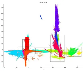
To empirically evaluate greedy PBVI, we tested it on the problem of tracking either one or multiple people using a multi-camera system. The problem was extracted from a real-world dataset collected in a shopping mall (Bouma et al. 2013). The dataset was gathered over 4 hours using 13 CCTV cameras. Each camera uses aFPDW pedestrian de-tector (Doll´ar, Belongie, and Perona 2010) to detect people in each camera image and in-camera tracking (Bouma et al. 2013) to generate tracks of the detected people’s move-ment over time. The dataset thus consists of 9915 tracks, each specifying one person’sx-y position throughout time. Figure 2 shows sample tracks from all of the cameras.
To address the blowup in the size of the state space for multi-person tracking, we use a variant oftransfer planning (Oliehoek, Whiteson, and Spaan 2013). We divide the multi-person problem into severalsourceproblems, one for each person, and solve them independently to computeVt(b) =
P
Vi(bi), where Vi(bi) is the value of the current belief bi about thei-th person’s location. ThusVti(bi)only needs to be computed once, by solving POMDP of the same size as that in the single-person setting. During action selection, Vt(b)is computed using the currentbifor each person.
As baselines, we tested against regular PBVI andmyopic versions of both greedy and regular PBVI that compute a policy assumingh = 1and use it at each timestep. More details about the experiments can be found in the extended version (Satsangi, Whiteson, and Oliehoek 2014).
[image:6.612.380.514.57.172.2]Figure 3 shows runtimes under different values of N and K. Since multi-person tracking uses the value func-tion obtained by solving a single-person POMDP, single and
Figure 2: Sample tracks for all the cameras. Each color rep-resents all the tracks observed by a given camera. The boxes denote regions of high overlap between cameras.
[image:6.612.335.536.345.439.2]multi-person tracking have the same runtimes. These results demonstrate that greedy PBVI requires only a fraction of the computational cost of regular PBVI. In addition, the dif-ference in runtime grows quickly as the action space gets larger: forN = 5andK= 2greedy PBVI is twice as fast, while forN = 11, K = 3it is approximately nine times as fast. Thus, greedy PBVI enables much better scalability in the action space.
Figure 3: Runtimes for the different methods.
Figure 4, which shows the cumulative reward under dif-ferent values of N and K for single-person (top) and multi-person (bottom) tracking, verifies that greedy PBVI’s speedup does not come at the expense of performance, as greedy PBVI accumulates nearly as much reward as regu-lar PBVI. They also show that both PBVI and greedy PBVI benefit from non-myopic planning. While the performance advantage of non-myopic planning is relatively modest, it increases with the number of cameras and people, which suggests that non-myopic planning is important to making active perception scalable.
per-Figure 4: Cumulative reward for single-person (top) and multi-person (bottom) tracking.
son and the red line plots the max of the agent’s belief. The difference in fluctuation in belief is evident from the figure as the max of the belief often drops below 0.5 for the myopic policy but rarely does so for the non-myopic policy.
Related Work
Dynamic sensor selection has been studied in many con-texts. Most work focuses on either open-loop or myopic so-lutions, e.g., (Kreucher, Kastella, and Hero 2005; Williams, Fisher, and Willsky 2007; Joshi and Boyd 2009). By con-trast, our POMDP-approach enables a closed-loop, non-myopic approach that can lead to better performance when the underlying state of the world changes over time.
Spaan (2008) and Spaan and Lima (2009) also consider a POMDP approach to dynamic sensor selection. However, they apply their method only to small POMDPs without ad-dressing scalability with respect to the action space. Such scalability, which greedy PBVI makes possible, is central to the practical utility of POMDPs for sensor selection. Other work using POMDPs for sensor selection (Krishnamurthy and Djonin 2007; Ji, Parr, and Carin 2007) also does not consider scalability in the action space. Krishnamurthy and Djonin (2007) consider a non-standard POMDP in which, unlike in our setting, the reward is not linear in the belief.
In recent years, applying greedy maximization to sub-modular functions has become a popular and effective ap-proach to sensor selection (Krause and Guestrin 2005; 2007). However, such work focuses on myopic or fully ob-servable settings (Kumar and Zilberstein 2009) and thus does not enable the long-term planning required to cope with dynamic state in a POMDP.
Adaptive submodularity(Golovin and Krause 2011) is a
0 10 20 30 40 50 60 70 80 90 100 0
0.2 0.4 0.6 0.8 1
Timestep
Max of belief
Max of belief Position of person covered by chosen camera Non−myopic
0 10 20 30 40 50 60 70 80 90 100
0 0.2 0.4 0.6 0.8 1
Timestep
Max of belief
[image:7.612.59.290.48.286.2]Max of belief Position of person covered by chosen camera Myopic
Figure 5: Behaviour of myopic vs. non-myopic policy.
recently developed extension that addresses these limitations by allowing action selection to condition on previous obser-vations. However, it assumes a static state and thus cannot model the dynamics of a POMDP across timesteps. There-fore, in a POMDP, adaptive submodularity is only applica-ble within a timestep, during which state does not change but the agent can sequentially add sensors to a set. In princi-ple, adaptive submodularity could enable this intra-timestep sequential process to be adaptive, i.e., the choice of later sen-sors could condition on the observations generated by earlier sensors. However, this is not possible in our setting because we assume that, due to computational costs, all sensors must be selected simultaneously. Consequently, our analysis con-siders only classic, non-adaptive submodularity.
To our knowledge, our work is the first to establish the submodularity of POMDP value functions for dynamic sen-sor selection POMDPs and thus leverage greedy maximiza-tion to scalably compute bounded approximate policies for dynamic sensor selection modeled as a full POMDP.
Conclusions & Future Work
[image:7.612.342.550.60.291.2]One avenue for future work includes quantifying the er-ror bound betweenV˜G
t (b)andV˜t∗(b), as our current results (Theorem 5) show only that it is bounded. We also intend to consider cases where its possible to sequentially process in-formation from sensors and thus integrate our approach with adaptive submodularity.
Acknowledgements
We thank Henri Bouma and TNO for providing us with the dataset used in our experiments. We also thank the STW User Committee for its advice regarding active perception for multi-camera tracking systems. This research is sup-ported by the Dutch Technology Foundation STW (project #12622), which is part of the Netherlands Organisation for Scientific Research (NWO), and which is partly funded by the Ministry of Economic Affairs. Frans Oliehoek is funded by NWO Innovational Research Incentives Scheme Veni #639.021.336.
References
Araya, M.; Buffet, O.; Thomas, V.; and Charpillet, F. 2010. A POMDP extension with belief-dependent rewards. In Ad-vances in Neural Information Processing Systems, 64–72. Astr¨om, K. J. 1965. Optimal control of Markov deci-sion processes with incomplete state estimation. Journal of Mathematical Analysis and Applications10:174—-205. Bertsekas, D. P. 2007.Dynamic Programming and Optimal Control, volume II. Athena Scientific, 3rd edition.
Bouma, H.; Baan, J.; Landsmeer, S.; Kruszynski, C.; van Antwerpen, G.; and Dijk, J. 2013. Real-time tracking and fast retrieval of persons in multiple surveillance cameras of a shopping mall. InSPIE Defense, Security, and Sensing. International Society for Optics and Photonics.
Cover, T. M., and Thomas, J. A. 1991. Entropy, relative entropy and mutual information. Elements of Information Theory12–49.
Doll´ar, P.; Belongie, S.; and Perona, P. 2010. The fastest pedestrian detector in the west. InProceedings of the British Machine Vision Conference (BMVC).
Gilbarg, D., and Trudinger, N. 2001.Elliptic Partial Differ-ential Equations of Second Order. Classics in Mathematics. U.S. Government Printing Office.
Golovin, D., and Krause, A. 2011. Adaptive submodularity: Theory and applications in active learning and stochastic op-timization.Journal of Artificial Intelligence Research (JAIR) 42:427–486.
Ji, S.; Parr, R.; and Carin, L. 2007. Nonmyopic mul-tiaspect sensing with partially observable Markov deci-sion processes. Signal Processing, IEEE Transactions on 55(6):2720–2730.
Joshi, S., and Boyd, S. 2009. Sensor selection via con-vex optimization. Signal Processing, IEEE Transactions on 57(2):451–462.
Kaelbling, L. P.; Littman, M. L.; and Cassandra, A. R. 1998. Planning and acting in partially observable stochastic do-mains. Artif. Intell.101(1-2):99–134.
Krause, A., and Golovin, D. 2014. Submodular func-tion maximizafunc-tion. In Tractability: Practical Approaches to Hard Problems (to appear). Cambridge University Press. Krause, A., and Guestrin, C. 2005. Optimal nonmyopic value of information in graphical models - efficient algo-rithms and theoretical limits. In International Joint Con-ference on Artificial Intelligence (IJCAI).
Krause, A., and Guestrin, C. 2007. Near-optimal obser-vation selection using submodular functions. In National Conference on Artificial Intelligence (AAAI), Nectar track. Kreucher, C.; Kastella, K.; and Hero, III, A. O. 2005. Sen-sor management using an active sensing approach. Signal Process.85(3):607–624.
Krishnamurthy, V., and Djonin, D. V. 2007. Structured threshold policies for dynamic sensor scheduling—a par-tially observed Markov decision process approach. Signal Processing, IEEE Transactions on55(10):4938–4957. Kumar, A., and Zilberstein, S. 2009. Event-detecting multi-agent MDPs: Complexity and constant-factor approxima-tion. InProceedings of the Twenty-First International Joint Conference on Artificial Intelligence, 201–207.
Lovejoy, W. S. 1991. Computationally feasible bounds for partially observed Markov decision processes. Operations Research39(1):pp. 162–175.
Monahan, G. E. 1982. A survey of partially observable Markov decision processes: Theory, models, and algorithms. Management Science28(1):pp. 1–16.
Nemhauser, G.; Wolsey, L.; and Fisher, M. 1978. An analy-sis of approximations for maximizing submodular set func-tions—i. Mathematical Programming14(1):265–294. Oliehoek, F. A.; Whiteson, S.; and Spaan, M. T. J. 2013. Ap-proximate solutions for factored Dec-POMDPs with many agents. InAAMAS13, 563–570.
Pineau, J.; Gordon, G. J.; and Thrun, S. 2006. Anytime point-based approximations for large POMDPs. Journal of Artificial Intelligence Research (JAIR)27:335–380. Satsangi, Y.; Whiteson, S.; and Oliehoek, F. A. 2014. Ex-ploiting submodular value functions for faster dynamic sen-sor selection: Extended version. Technical Report IAS-UVA-14-02, University of Amsterdam, Informatics Insti-tute.
Smallwood, R. D., and Sondik, E. J. 1973. The optimal control of partially observable Markov processes over a fi-nite horizon.Operations Research21(5):pp. 1071–1088. Spaan, M. T. J., and Lima, P. U. 2009. A decision-theoretic approach to dynamic sensor selection in camera networks. InInt. Conf. on Automated Planning and Scheduling, 279– 304.
Spaan, M. T. J. 2008. Cooperative active perception us-ing POMDPs. InAAAI 2008 Workshop on Advancements in POMDP Solvers.