STATISTICAL
I
NFERENCE
FOR MOVEMENT
BEHAVIO
UR
USING ANIMAL TRACKING
DATA
by
Robin
B
arbara
Th
o
m
so
n
,
B
.Sc. (
Z
ool),
B
.Sc.
H
ons (
Z
oo
l
), M.Sc.(Appl.
Maths),
Un
iv
ersity
of Cape
T
own
Submitted in fulfilment of the requirements for the Degree of Doctor of Philosophy
D
epartment of
Mathematics
Unive
rsi
ty of
Ta
sman
i
a
Octob
er,
2008
I declare that this thesis contains no material which has been accepted for a degree or diploma by the University or any other institution, except by way of background information and duly acknowledged in the thesis, and that, to the best of my knowledge and belief, this thesis contains no material previously published or written by another person, except where due acknowledgement is made in the text of the thesis.
Signed:
--
~
-'----=---
Robin Barbara ThomsonThis thesis may be made available for loan and limited copying in ac-cordance with the Copyright Act 1968.
Signed:
--
-
~
-'---
Robin Barbara Thomson
ABSTRACT
Satellite tracking provides an opportunity to learn about how animals choose to move and about the covariates of movement. Quantitative methodology for this problem has lagged behind the remote sensing technology that provides both ani-mal tracks and covariate information. A statistical framework capable of providing appropriate hypothesis testing has to couple very different types of data: highly au-tocorrelated time series of observed locations (the track), with 2-dimensional maps of " covariate data. In addition, animals respond to internal motivations, representable only as theorised motivations. Behaviour is likely to be highly complex and to be only approximately understood so that process error cannot be ignored. Observa-tion error should be accounted for separately from process error because longitude is typically more difficult to estimate than latitude, and because estimates of ob-servation error are sometimes available. State space models account separately for observation and process errors, and model the serial correlation inherent in tracks. State space models offer great flexibility, nevertheless, the means of incorporating diverse movement behaviours and covariate information is not immediately clear. , Traditionally, these models require that time series be equally spaced in time (sel-dom the case with observed tracks) and they have presented substantial difficulties in inference.
ACKNOWLEDGEMENTS
TABLE OF CONTENTS
TABLE OF CONTENTS
LIST OF TABLES
LIST OF FIGURES
1 GENERAL INTRODUCTION
1.1 Track data . . . .
1.2 Covariates and hypotheses of behaviour
1.3 Modelling framework .
1.4 Hypothesis selection
1.5 Thesis structure . . .
2 LITERATURE REVIEW
2.1 Abstract . . .
2.2 Introduction .
2.2.1 Definitions
2.3 Collecting track data .
2.3.1 Direct observation
2.4
2.3.2 Aquatic acoustic listening stations
2.3.3 Radio and acoustic tracking . . . .
2.3.4 Archival tags and Satellite trackers .
Quantitative methods . .
2.4.1 Empirical methods
2.4.2 Random walks and advection-diffusion models
2.4.3 Bulk transfer process . . .
i
vi
viii
1
3
4
6
10
10
13
13
14
17
18
18
19
19
20
21
21
24
TABLE OF CONTENTS
2.4.4 IBMs
...
2.4.5 Time series models and state space models
2.4.6 Discrete states and hidden Markov models .
2.5 SSMs in more detail
2.5.1 Nomenclature .
2.5.2 Model framework .
2.5.3 Hierarchical SSMs
2.5.4 Inference for SSMs
2.5.5 SSMs in wildlife population and movement modelling
2.6 Monte Carlo methods
....
2.6.l Importance samplers .
2.6.2 Markov Chain Monte Carlo
2.6.3 Convergence
2.7 Model comparison
2.7.1 Methods ..
2.7.2 Movement studies
2.8 This study . . .
3 FRAMEWORK FOR ANIMAL MOVEMENT BEHAVIOUR
3.1 Abstract . . .
3.2 Introduction .
3.3 Methods . . .
3.3.1 Observation equation
3.3.2 State equation
....
3.3.3 Modelling behaviour using advection
3.3-.4 Posterior, Likelihood, Priors and Initial conditions
3.3.5 Conditional distributions
3.3.6 MCMC
. . .
3.3.7 Simulation scenarios
3.4 Results . . .
3.5 Discussion .
4 CHANGING BEHAVIOUR THROUGH TIME
4.1 Abstract . . . .
TABLE OF CONTENTS iii
4.2 Introduction. 82
4.3 Methods . . . 84
4.3.1 The model 84
4.3.2 Priors
...
864.3.3 The posterior 86
4.3.4 Conditional distributions 87
4.3.5 Simulation and estimation . 91
4.4 Results . . . 93
4.5 Discussion . 102
5 BAYESIAN MODEL COMPARISON 104
5.1 Abstract . . . 104
5.2 Introduction. 105
5.3 Methods . . . 109
5.3.1 Bayes factor . 109
5.3.2 Monte Carlo estimation 110
5.3.3 Harmonic Mean
....
1115.3.4 Chib's Candidates Method 111
5.3.5 DIC
. . .
1185.3.6 MCMC and convergence. 120
5.3.7 Spread of model comparison measures 121
5.3.8 Simulation and estimation . 121
5.4 Results . . . 124
5.5 Discussion . 127
6 HARMONIC MEAN ESTIMATOR INAPPROPRIATE 129
6.1 Abstract . . . 129
6.2 Introduction: Bayes factor and the marginal likelihood . 130
6.3 Methods . . . 131
6.3.1 Importance sampling the marginal likelihood 131
6.3.2 Simulation 132
6.4 Simulation results 133
6.5 Discussion . 135
TABLE OF CONTENTS iv
7 USING LAPLACE'S EQUATION TO MOVE AROUND
OBSTA-CLES 138
7.1 Abstract . . . 138
7.2 Introduction . 139
7.3 Methods . . . 142
7.3.1 Heat diffusing through a grid 142
7.3.2 Boundary conditions . . . 143
7.3.3 Advection from temperature gradient 144
7.3.4 Simulated landscapes: central landmass 144
7.3.5 Simulated landscape: South Australia 147
7.3.6 Simulated movement . 148
7.4 Results . . . 150
7.4.1 Central landmass . 150
7.4.2 South Australian sharks 153
7.5 Discussion . . . 158
8 APPLICATION TO WHITE SHARK TRACKS 159
8.1 Abstract . . . 159
8.2 Introduction . 160
8.3 Methods . . . 162
8.3.1 Data. 162
8.3.2 Simulated tracks 165
8.3.3 Advection fields . 167
8.3.4 Movement model and estimation 173
8.3.5 Time and latent locations 175
8.3.6 DIC and MCMC 175
8.4 Results . . . 176
8.4.l Simulated tracks 176
8.4.2 Convergence: movement close to land 177
8.4.3 Estimation using simulated tracks 181
8.4.4 Estimation using observed tracks 185
8.5 Discussion . . . 189
TABLE OF CONTENTS
9 GENERAL CONCLUSION
9.1 Future work . . . . . . . .
10 SYMBOLS USED IN THIS THESIS
11 POSTERIOR AND CONDITIONALS
11.l Conditional distributions . . . .
11.2 Posterior distribution . . . .
12 GAMMA CONDITIONAL DISTRIBUTION
v
195
198
201
205
205
206
210
13 MULTIVARIATE NORMAL CONDITIONAL DISTRIBUTION 212
14 WISHART CONDITIONAL DISTRIBUTION
15 R CODE FOR FIGURE
REFERENCE LIST
217
220
LIST OF TABLES
3.1 'True' parameter values used to simulate tracks, are shown. Note that the shape a and rate b parameters of the gamma distribution can be calculated from the distribution's mean µ and variance a2 using the formulae a = µ2
/a
2 and b = µ/a2. The gamma prior distributions are expressed both in terms of shape a and rate b, and mean and variance . . . .
3.2 Priors used for estimation. Note that the shape a and rate b pa-rameters of the gamma distribution can be calculated from the dis-tribution's mean µ and variance a2 using the formulae a = µ2 / a2
64
and b = µ/a2• The gamma prior distributions are expressed both in terms of shape a and rate b, and also mean and variance. . . 65
4.1 Description of four advection scenarios that use different functional forms for the changes in the advection coefficients B with time, and different advection fields. . . 91
4.2 Parameter values and dimensions used to simulate tracks. . . 93
4.3 Priors used in estimation. Note that the shape a and rate b param-eters of the gamma distribution can be calculated from the distri-bution's mean µ and variance a2 using the formulae a
= µ
2/ a2 and b = µ / a2
. The gamma prior distributions are expressed both in terms of shape a and rate b, and also mean and variance. . . 94
4.4 Average estimated (co)variance
(rB)-1.
For every one of the 100 OOO posterior draws, the coval'iance between the vectors B1 and B2 was estimated, and the average over these 100 OOO covariances is given in this table. Results are given for the four pairs of advections that represent the four simulation scenarios listed in Table 4.1. . . 995.1 Scale presented by Kass and Raftery (1995) after Jeffreys (1961) for interpretation of the Bayes factor (B12) for model H1 compared with model H2. . . 109
5.2 Parameter values and dimensions used in simulating the track. 122
5.3 Priors used for estimation. . . 123
LIST OF TABLES
5 .4 Mean (and coefficient of variation c. v.) estimated marginal likeli-hoods and the Bayes factor for two competing models, one using the correct and the other an incorrect advection field. Estimation was by the multiple block (CJ), and single block (CJl) Chib & Jeliazkov (2001) methods and the harmonic mean method (HM). The final column gives an evaluation of the evidence in favour of the correct model. Results are shown for the three estimation scenarios detailed in Table 5.3, which use different priors for the precision parameters
vii
Tx and Ty. . . 126
5.5 Deviance Information Criterion (DIC) for the three estimation sce-narios detailed in Table 5.3. . . 126
6.1 Showing 5, 50 and 95 percentiles from 100 repeated estimations of the error in the marginal likelihood (m(y) - m(y)). Each estimation m(y) used 1000 OOO draws from the posterior. Results are shown for four values of n for the harmonic mean and the RIS estimators. . . . 135
8.1 Parameter values and settings used when simulating four shark tracks. The starting locations, time steps and number of locations were those observed when tracking four white sharks in South Australia. 167
8.2 Prior distributions used in the movement model. . . 174
8.3 The mean and standard deviation (in parentheses) of five repeated calculations of the deviance information criterion DIC for the alter-native hypotheses, using simulated tracks. The 'All' hypothesis com-bined the three advection fields 'Depth', 'Distance' and 'Direction'. An asterisk indicates the lowest DIC value in each column. . . 182
8.4 The mean and standard deviation (in parentheses) of five repeated calculations of the deviance information criterion DIC for the alter-native hypotheses, using observed tracks. The 'All' hypothesis com-bined the three advection fields 'Depth', 'Distance' and 'Direction'. An asterisk indicates the lowest DIC value in each column. . . 185
8.5 Posterior mean parameter values for four movement hypotheses for each of three observed shark tracks. . . 186
LIST OF FIGURES
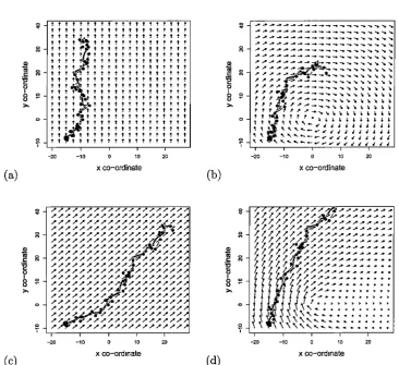
3.1 Advection fields, or combinations of fields, for the four simulations used to generate tracks; (a) a single northwards flow; (b) a single clockwise gyre; (c) combined northwards and eastwards flows; and (d) combined northwards flow with clockwise gyre. Plots (c) and (d) show only the vector sum of the two fields that are used in these scenarios. The path x that was simulated using each (set) of fields is shown in grey, with a large black dot indicating the first location. The observed locations (track) y are shown as black, joined, dots. . . 63 3.2 Results from 200 OOO MCMC draws from the posterior of the
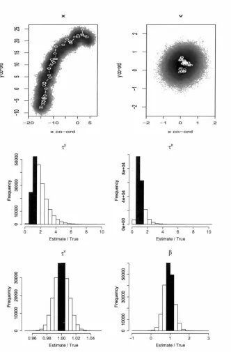
esti-mation model that uses northerly advection (scenario 1), applied to the track generating using this same advection. States are shown as Cartesian coordinates (the simulated values as open circles joined by white lines and the MCMC draws as a density plot). Parameters are shown as a fraction of their true values so that a correct value is given as 1; the bars that span this value are shaded in black. . . 68
3.3 Results from 200 OOO MCMC draws from the posterior of the es-timation model that uses a clockwise gyre (scenario
2),
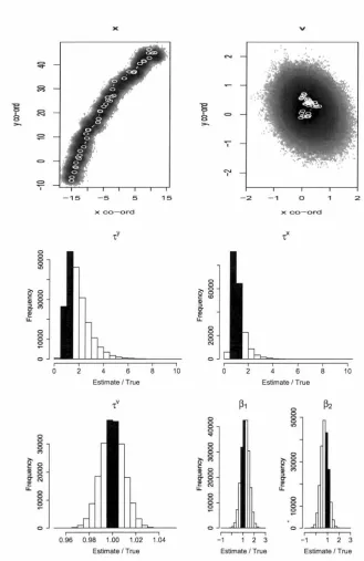
applied to the track generating using this same advection. States are shown as Cartesian coordinates (the simulated values as open circles joined by white lines and the MCMC draws as a density plot). Parameters are shown as a fraction of their true values so that a correct value is given as 1; the bars that span this value are shaded in black. . . 693.4 Results from 200 OOO MCMC draws from the posterior of the esti-mation inodel that uses northerly advection combined with easterly advection (scenario 3), applied to the track generating using these same advections. States are shown as Cartesian coordinates (the simulated values as open circles joined by white lines and the MCMC draws as a density plot). Parameters are shown as a fraction of their true values so that a correct value is given as 1; the bars that span this value are shaded in black. . . 70
LIST OF FIGURES
3.5 Results from 200 OOO MCMC draws from the posterior of the esti-mation model that uses northerly advection combined with a gyre (scenario 4), applied to the track generating using these same ad-vections. States are shown as Cartesian coordinates (the simulated values as open circles joined by white lines and the MCMC draws as a density plot). Parameters are shown as a fraction of their true values so that a correct value is given as 1; the bars that span this
ix
value are shaded in black. . . 71
3.6 Results from 200 OOO MCMC draws from the posterior of the estima-tion model that uses northerly advecestima-tion (scenario 1), applied to the track generating using this same advection. The prior for rY had a mean value five times the true value. States are shown as Cartesian coordinates (the simulated values as open circles joined by white lines and the MCMC draws as a density plot). Parameters are shown as a fraction of their true values so that a correct value is given as 1; the bars that span this value are shaded in black. . . 73
3. 7 Results from 200 OOO MCMC draws from the posterior of the estima-tion model that uses northerly advecestima-tion (scenario 1), applied to the track generating using this same advection. The prior for rx had a mean value five times the true value. States are shown as Cartesian coordinates (the simulated values as open circles joined by white lines and the MCMC draws as a density plot). Parameters are shown as a fraction of their true values so that a correct value is given as 1; the bars that span this value are shaded in black. . . 7 4
3.8 Results from 200 OOO MCMC draws from the posterior of the estima-tion model that uses northerly advecestima-tion (scenario 1), applied to the track generating using this same advection. The prior for rv had a mean value five times the true value. States are shown as Cartesian coordinates (the simulated values as open circles joined by white lines and the MCMC draws as a density plot). Parameters are shown as a fraction of their true values so that a correct value is given as 1; the bars that span this value are shaded in black. . . 75
3.9 Results from 200 OOO MCMC draws from the posterior of the esti-mation model that uses northerly advection (scenario 1), applied to · the track simulated using a combination of northerly advection and a gyre (scenario 4). States are shown as Cartesian coordinates (the simulated values as open circles joined by white lines and the MCMC draws as a density plot). Parameters are shown as a fraction of their true values so that a correct value is given as 1; the bars that span this value are shaded in black. . . 76
LIST OF FIGURES
4.2 Estimation results for scenario 1, which uses linearly declining adher-ence to a northerly advection field combined with linearly increasing adherence to a northeasterly field. The x and v plots show the true values as white, open circles and the 100 OOO MCMC draws as a den-sity plot. The precision parameters TY, Tx and Tv are shown as a fraction of their true values, so that a correct value is given as 1; the
x
bars that span this value are shaded in black. . . 95
4.3 Estimation results for scenario 2, which uses linearly declining adher-ence to a southerly advection field combined with linearly increasing adherence to a gyre. The x and v plots show the true values as white, open circles and the 100 OOO MCMC draws as a density plot. The precision parameters TY, Tx and Tv are shown as a fraction of their true values, so that a correct value is given as 1; the bars that span this value are shaded in black. . . 96
4.4 Estimation results for scenario 3, which uses an S-shaped declining adherence to a northerly advection field combined with an S-shaped increasing adherence to a northeasterly field. The x and v plots show the true values as white, open circles and the 100 OOO MCMC draws as a density plot. The precision parameters TY, Tx and Tv are shown as a fraction of their true values, so that a correct value is given as 1; the bars that span this value are shaded in black. . . 97
4.5 Estimation results for scenario 4, which uses an S-shaped declining adherence to a southerly advection field combined with an S-shaped increasing adherence to a gyre. The x and v plots show the true values as white, open circles and the 100 OOO MCMC draws as a density plot. The precision parameters TY, Tx and Tv are shown as a fraction of their true values, so that a correct value is given as 1; the bars that span this value are shaded in black. . . 98
4.6 Marginal posteriors for the coefficients B for advection scenarios 1-4, listed in Table 4.1. The posterior median is indicated by a white line, a 953 credibility interval by thin black lines, and shading indicates posterior density. The true values used in the simulation are indicated by a thick black line. . . 100
5.1 Advection fields for (a) the simulation and (b) the incorrect alterna-tive hypothesis. The simulated path x is shown as thick grey line and the starting point for the path x1 as a large black dot. The simulated observations y are shown as small black dots. . . 122
LIST OF FIGURES
6.1 Error in the estimated log marginal likelihood for an increasing nwn-ber of draws from the posterior distribution is shown. Results are shown for four data sample sizes n. The harmonic mean (HM), and
xi
the Reciprocal Importance Sampling (RIS) estimators are shown. . . 134
7.1 Advection fields generated from a temperature gradient around a sim-ulated landmass that dominates the landscape. A 500 by 500 cell grid was used. Boundary conditions were (a) Dirichlet land and grid; (b) Dirichlet land and Neumann grid; and (c) Neumann land and Dirich-let grid. Colours indicate temperature on a log scale (hottest cells are red, coolest green). . . 145
7 .2 Advection fields calculated from a temperature gradient around a relatively small central landmass. A 500 by 500 cell grid was used. White indicates land, colours indicate temperature on a log scale (hottest cells are red, coolest green). Boundary conditions were (a) Dirichlet land and grid; (b) Dirichlet land and Newnann grid; and
(c) Newnann land and Dirichlet grid. . . 146
7.3 Part of the gulf region of South Australia, grey indicates land and white ocean. . . 147
7.4 Advection directly towards the Neptune Islands . . . 148
7.5 Advection fields for part of South Australia calculated from a tem-perature gradient. A 500 by 500 cell grid is used. White indicates land, colours indicate temperature on a log scale (hottest cells are red, coolest green). Boundary conditions were (a) Dirichlet land and grid; (b) Dirichlet land and Newnann grid; and (c) Neumann land and Dirichlet grid. . . 149
7.6 Paths taken by ten marine animals moving towards a target on the other side of a landmass that dominates the landscape. Boundary conditions were (a) Dirichlet land and grid; (b) Dirichlet land and Neumann grid; and (c) Neumann land and Dirichlet grid. Colours indicate temperature on a log scale (hottest cells are white, coolest red) . . . 152
7.7 Paths taken by ten marine animals moving towards a target on the other side of a landmass. White indicates land, colours indicate tem-perature on a log scale (hottest cells are white, coolest red). Bound-ary conditions were (a) Dirichlet land and grid; (b) Dirichlet land and Neumann grid; and (c) Newnann land and Dirichlet grid. . . 154
LIST OF FIGURES
7.9 Paths taken by ten simulated marine animals moving along the South Australian coast towards the Neptune Islands. Boundary conditions were (a) Dirichlet land and grid; (b) Neumann land and grid; and (c) Dirichlet land and Neumann grid. The random walk used a variance of a2
= 1
2. Colours indicate temperature on a log scale (hottest cellsxii
are white, coolest red). . . 156
7.10 Paths taken by ten simulated marine animals moving along the South Australian coast towards the Neptune Island. Boundary conditions were (a) Dirichlet land and grid; (b) Neumann land and grid; and (c) Dirichlet land and Neumann grid. The random walk used a variance of a2
= 3
2. Colours indicate temperature on a log scale (hottest cells are white, coolest red). . . 1578.1 Sections of observed tracks for four white sharks (identified by name and number) tagged off South Australia. The track is white and the first location is a black triangle. Bathymetry is indicated by shading and by contours, which are shown every 20m up to a depth of 200m. 163
8.2 Smoothed bathymetric data were used to calculate advection fields (white arrows) representing navigation by following the 80m iso-bath and a preference for travel (a) eastwards, or (b) westwards. Bathymetry is indicated by shading and by contours, which are shown every 20m up to a depth of 200m. . . 170
8.3 Unsmoothed bathymetric data results in somewhat erratic advection fields (white arrows) representing navigation by following the 80m isobath and a preference for travel (a) eastwards, or (b) westwards. Bathymetry is indicated by shading and by contours, which are shown every 20m up to a depth of 200m. . . 170
8.4 Whit'e arrows indicate advection fields representing a preference for remaining 50km from the coast and for moving (a) eastwards, and (b) westwards. Bathymetry is indicated by shading and by contours, which are shown every 20m up to a depth of 200m. . . 172
8.5 White arrows indicate advection fields representing a preference for travel (a) southeasterly in Spencer Gulf and northeasterly outside of it, and (b) northeasterly in Spencer Gulf and southeasterly outside of it. Bathymetry is indicated by shading and by contours, which are shown every 20m up to a depth of 200m. . . 173
LIST OF FIGURES
8.7 Simulated tracks (shown as connected white dots) that used the ob-served start location, number of locations and time steps obob-served for four white sharks (identified by name and number) tagged off South Australia. The simulated path is shown as black dots, the 'ob-served' locations are white dots joined by a white line. The tracks were simulated using the 'Depth' advection field (shown as white ar-rows). Bathymetry is indicated by shading and by contours, which
xiii
are shown every 20m up to a depth of 200m. . . 178
8.8 Trace plots (the x-axis shows the MCMC iteration number) for the longitude of the fifth location x5 1 in the path of the observed track for
shark 1, Sam (a) before thinning, and (b) after thinning. Results are presented for the model that uses the 'Depth' advection field. The selection of this particular component of the x matrix was arbitrary. 180
8.9 Trace plots (the x-axis shows the MCMC iteration number) for the longitude of the fifth location x51 in the path of (a) the simulated
track, and (b) the observed track for shark 4, Michael. Results are presented for the model that uses the 'Depth' advection field. The selection of this particular component of the x matrix was arbitrary. 181
8.10 Credibility intervals (953) for parameters estimated from simulated tracks. The 53 and 953-iles are marked by squares, the median by a dash, and the mean by an open circle. The estimated values are divided by their true (simulation) value so that the grey horizontal line at 1 indicates a correct estimate. The true value for
/3
2 and {33 is zero (marked by a dotted line), so that their estimates were divided by the true value for/31. . . . . . . .
183CHAPTER
1
GENERAL INTRODUCTION
Understanding animal movements and identifying the factors that influence these movements has long been a goal of ecological research (Turchin, 1998; Okubo, 1980;
Okubo
&
Levin, 2001). Better understanding of animal movements can improve natural resource management through mitigation of unwanted bycatch (Broekhuizenet al. , 2003), guiding the selection of new protected areas (Maury
&
Gascuel, 1999; van Vuren, 1998), and forecasting the impact of climate change on populationdis-tributions (Bowler
&
Benton, 2005).Information on the movements of animals can be obtained from a number of sources,
even examination of their tissues. Otolith microchemistry, for example, may reveal
which bodies of water a fish has resided in during its life, by the isotopes found in sections of its ear bones (Elsdon
&
Gillanders, 2003). Mitochondrial and nuclearDNA investigation revealed that while male white shark DNA is shared between
Australia and Africa, female genetic material is not, indicating that males travel
across the Indian ocean whereas females are resident (Pardini et al. , 2001). How-ever, the most powerful techniques for revealing animal movements are tagging and
tracking methods. A single track of a female white shark showed that she travelled from South Africa to· Australia, and subsequent photo-identification that she ~e turned to South Africa. Thus the conclusions of the genetic study were overturned:
although only male genetic material is exchanged it is the females that travel to collect it and carry it back home (Bonfil et al. , 2005).
Most statistical methods require large numbers of independent observations from
which inferences may be drawn. A single track, composed of non-independent obser-vations taken from a single individual, is unsuitable for application of most statistical
methods other than those of time series methodology (Chatfield, 2004). Here the
2
track itself, a sequence of serially correlated observations, is the time series.
Further difficulties must be overcome: time series methods have been developed primarily for identifying patterns evident within a long series of sequential observa-tions, so that this pattern can be forecast into the future. The underlying reasons
for this pattern, and its covariates, are often of secondary importance. An annual seasonal oscillation, for example, may be evident and can be projected into future
years. In order to detect such a seasonal pattern, observations will be required from
at least two, usually many more, past years. Seasonal patterns are very likely to occur in animal movement behaviour, but animal tracking data are usually
mea-sured in weeks or months, not years. Such tracks are therefore unlikely to yield
repeated observations of past patterns, but rather a single instance, or perhaps
only a part of, a particular pattern. Tracks must therefore be understood, not by recognising a repeating pattern, but rather by identifying the external covariates or
internal motivations that drive the moving animal, so that future movements may be forecast using future projections of these covariates (such that those forecast by
oceanographic or meteorological models). Time series techniques typically do not make use of large datasets of covariate information because such correlates of the
repeating patterns found in the data are of secondary importance. In the case of
animal tracking data, however, these covariates are of importance.
A family of time series methods is presented in this thesis that is capable of combin-ing covariate information with observed tracks. Movement behaviour, as a response
to measured environmental variables or to theorized internal states, is hypothesized
by the investigator. Alternative behavioural hypotheses are formulated, and the
support given to each by an observed track is measured. As further tracks are col-lected, and hypotheses tested, theories of movement behaviour may be refined. In
this way, it is hoped, understanding of the, no doubt, complex movement behaviour of animals will be gained incrementally.
Databases of satellite tracks are growing around the world (Coyne & Godley, 2005)
and statistical methods capable of using these tracks for inference about movement behaviour are badly needed. It is not expected that any theory of animal behaviour,
implemented as a statistical model, will be exactly correct. Instead, it is hoped that the process of model selection and model building will facilitate incremental learn-ing regardlearn-ing the movement behaviour of animals. As Box (1979) famously said 'all models are wrong but some are useful'. This thesis presents a statistical model for animal movement behaviour that can be used together with methods of model
1.1. TRACK DATA 3
movement behaviour. Hypothesized movement behaviours are unlikely to exactly replicate the motivations of a moving animal, instead the aim of this work is to pro-vide a tool that measures the support given by track data to hypotheses of movement
behaviour so that by discarding and refining hypotheses a greater understanding of movement behaviour can be gained incrementally.
This chapter briefly discusses the four elements required for this process: track
data; covariate information; a model capable of using a hypothesis of movement
behaviour, together with candidate covariate information, to simulate the track of a moving animal; and a means of measuring the support given by an observed track
to the model generated simulation. Finally, an outline of the thesis is given.
1.1 Track data
Track data have been collected by direct observation (by eye or using a camera) or
through radio- (or sonar-) tracking, either by an investigator physically following a tagged animal, or through arrays of monitoring devices placed in the region in
which an animal moves. More recently, however, the tracking of moving animals, even those that travel great distances across oceans or that fly over mountain ranges,
has been made easier by advances in satellite tracking technology (Priede
&
French,1991; White
&
Garrott, 2006). Researchers no longer have to follow along after the animals they are tracking, holding radio-receivers. Satellites and GPS systemspro-vide accurate, frequent position fixes for animals that move on the surface of the land
or ocean. Satellite communication is not possible for those that move beneath
wa-ter, seldom or never surfacing. For these animals, archival tags are required. These store information, including light-level data from which location may be inferred,
and must either be retrieved or after a pre-determined time, detach themselves from
their host animal, float to the surface, and send their information to satellites. This
.
.
technology, although expensive, is now widely used. Coyne&
Godley (2005) report that between 1995 and 2005 a five-fold increase was reported in the numbers ofanimals tracked by the Argos satellite system. However, due to the expense of this technology, available tracks typically represent only a small number of individuals from any population.
1.2. COVARJATES AND INPOTHESES OF BEHAVIOUR 4
hence, has more to do with its present location and its speed of travel than its ulti-mate destination. Satellite tracked locations are not equally-spaced in time because the tags communicate with satellites when possible, they cannot do so when the
animal to which they are attached is submerged, or inside a rocky cave, or when no satellites are overhead (Priede & French, 1991). Radio-tracking is also likely to
provide irregularly-timed location estimates and even archival tags, which record information at regular intervals, are only able to provide information from which
location can be estimated at dawn and dusk, provided the animal is not diving too
deeply and cloud cover is not too great, so that even these tags may provide some-what irregularly-timed locations.
The error structure of observed track locations can be somewhat unusual. The
Argos system grades every location that it provides into one of six error classes. The error structure associated with each class has been shown to be normally
dis-tributed but ellipsoidal, having greater variance in longitude than in latitude; the
extent of this variance differs among error classes (Vincent et al. , 2002). Tracks de-rived from archival tag light level information also show greater errors in longitude than in latitude (Sibert et al. , 2003).
1.2
Covariates and hypotheses of behaviour
The satellite technology used to collect track data has also facilitated the
collec-tion of environmental informacollec-tion. The MODIS system, for example, measures sea
surface temperature and colour for the oceans. Measurements of ocean height are used to infer movements of ocean currents. These data have been used to develop
accurate, mid-scale ocean and atmosphere models as well as maps of terrestrial
conditions (Campbell, 2006; Ryerson, 1998). Such environmental information is typically available in the form of 2- or 3-dimensional grids.
Moving animals may respond to particular environmental cues, for example, tuna appear to move so as to remain in waters of particular temperatures (Block et al. , 1998). Observed tracks of moving animals may contain cues that would allow
inves-tigators to infer which environmental variables are possible covariates of movement behaviour, and which are not.
One way of inferring whether an environmental variable is a determinant, or at
1.2. COVARIATES AND HYPOTHESES OF BEHAVIOUR 5
environmental information and to see, by eye, whether there seems to be any
corre-spondence. Most investigations will at least begin with an informal investigation of this sort, but scientific enquiry requires more rigorous, formal statistical testing of
hypotheses. Therefore, a statistical method is required that can relate two very dif-ferent sorts of information: tracks, and maps of environmental covariate information.
Of course, moving animals will not only respond to observed and observable
fea-tures of their environment, they will also respond to feafea-tures that investigators have
not observed, such as the presence of prey animals or conspecifics, and they will respond to internal motivations such as a desire to move to a spawning area during
a breeding season. Some of these behaviours might be included, implicitly, in a
model of movement behaviour, as random noise. More persistent behaviours, such as migration, will also have to be accounted for. The statistical model for movement
behaviour would therefore also need to incorporate behaviours that do not relate to
observed covariate information, such as migrations or movements towards spawning grounds.
It is envisioned that investigators wishing to use track data to make inferences about
the motivations for movement behaviour will form competing hypotheses. Some of these will relate to covariate information, others will identify areas towards, or away
from, which the animal is thought to move at particular times. The same covariate
information may be used, in different ways, by competing hypotheses that predict different responses. For example, it may be thought that a particular animal uses
the earth's magnetic field as a navigational aid. It may do this naively, moving
'up-stream' through the magnetic field until it finds an area that matches the magnetic
properties of the location towards which it wishes to move, or it may have a memory of the irregularities in the field between its starting point and target location and
may correct for these. It is also recognized that different hypotheses regarding the motivations of a moving animal may lead, indistinguishably, to similar theorized
behaviour. For example, a marine animal moving along the east coast of Australia
could be following a line of bathymetry, could be using the sounds of coastal waves to remain a particular distance from the coast, or could be maintaining an orientation with respect to the earth's main magnetic field. These factors appear to be almost perfectly correlated in this region, so that these three hypotheses are unlikely to be distinguishable using track data.
More than one of the behaviours discussed above could occur simultaneously - an aquatic animal may undertake a migration, navigating using the earth's magnetic
1.3. MODELLING FRAMEWORK 6
slowing down, perhaps to feed.
1.3 Modelling framework
Combined with present computing power, remotely sensed information gives
re-searchers the opportunity to investigate which of the measured variables of the
environment through which an animal moves, appear to affect its movement
be-haviour.
A numerical model capable of combining track data with hypotheses regarding
be-haviour (which may use covariate information) must couple very different types of information: tracks, maps of covariate data, and pure theory. In addition, the model
must be robust to responses to unobserved factors for which no specific theory is available, such as responses to other, untagged, animals. Movement behaviour is
likely to be highly complex and individuals are unlikely to all behave in the same manner. Theoretical models can therefore be expected to be significantly in error, so that process errors should be modelled. Observation errors should also be modelled;
track locations, even when collected using GPS enabled satellite tags, are imprecise. These observation errors must be unequal in latitude and longitude. Such a model
must also be able to account for the irregular time steps typical of non-archival tracking data. In addition, it would be useful to have the facility to estimate latent
(unobserved) locations. Long delays can occur between subsequent observed
loca-tions and, because the assumption is usually made that animals move in a straight line between observed locations, this can sometimes result in unrealistic behaviour.
For example, an aquatic animal may return a location estimate from one side of an
island or spit, and its next location from the opposite side, so that a straight-line
interpolation would indicate that it had crossed the land barrier. Even without an intervening barrier, the hypothesis of movement behaviour implemented by the
model might predict a more complicated path between two distant points than that given by a straight line. For these reasons, it would be desirable to have the ability
to include latent locations in a model of movement behaviour.
State space models (SSMs) provide a promising framework for overcoming these difficulties (Patterson et al. , 2007; Hilborn, 1990; Newman, 1998, 2000). SSMs
1.3. MODELLING FRAMEWORK 7
will model the track as a time series, therefore taking account of its inherent serial correlation. Each track would be modelled individually, therefore, data from a large number of individuals are not required. However, tracks from several individuals
can be combined in a hierarchical framework (Jansen et al. , 2003; Newman, 2000;
Newman
&
Lindley, 2006). Sibert et al. (2003) and Jansen et al. (2006) have shown that the unusual error structure of satellite tracking data can beaccommo-dated within an SSM framework.
Some challenges remain. SSMs represent time in a discrete fashion, giving the state
of a system at a series of equally spaced points in time. Satellite tracking provides data that are irregular as it relies on the animal surfacing and the tracker signalling
an overhead satellite. Others have applied SSMs to satellite tracking data by
'regu-larising' the data through calculation of some form of weighted average (Flemming et al. , 2006), by assuming that all observations occurring within a time step were
taken at the same time (Jansen et al. , 2006), or by interpolation (Tremblay et al. , 2006). Jansen et al. (2005) represent irregular time steps in the model itself through
the observation equation. Their observations of location are time-weighted averages
of an underlying regularly-timed series of unobserved locations (the state variables). As an alternative, this thesis presents an SSM framework in which locations are
ir-regularly spaced in time, and the duration of each time step is accounted for within
the model's state equation.
Published movement models applied to tracking data typically include only a single
potential covariate for movement, if any. Jansen et al. (2003) made the variance of the process errors a function of sea surface temperature (SST) so that turtles slowed
when they entered warmer water. Behaviour, not mediated by a covariate, has been included as a tendency to drift in a particular direction (Jansen et al. , 2005, 2006),
as switching between alternative parameter sets (Jansen et al. , 2005; Morales et al. ,
2004), or as deviation from a pre-specified route (Flemming et al. , 2006). However, behaviour is likely to result from a combination of all of these factors operating at
once, and perhaps a need to follow a navigational route as defined, for example, by landmarks, the earth's magnetic field or star patterns.
This thesis presents a method of representing movement behaviour as one or more advection fields that push the moving animal in particular directions. Separate models (co-models) use observed covariate information and theories on how and when animals choose to move, to generate 2-dimensional sets of advection forces.
num-1.3. MODELLING FRAMEWORK 8
ber of advection fields can be incorporated into the model - the overall direction of movement is given by a weighted, linear combination of advection forces.
The influence of the environment on the movements of the animal causes future loca-tions to be dependent on past localoca-tions (and the state of the environment at the past locations) so that the problem becomes highly nonlinear. In the past, the usefulness
of SSMs has been limited by difficulties in inference for nonlinear, and non-Gaussian,
forms of this model. Now Markov chain Monte Carlo (MCMC) methodology and current computing power offer release from these constraints (Buckland et al. , 2004; Newman
&
Lindley, 2006; Thomas et al. , 2005; Jansen et al. , 2003, 2005, 2006)although some challenges remain and this is an area of active research (Buckland et al. , 2004; Newman
&
Lindley, 2006). A great advance has been provided by the WinBUGs software (Spiegelhalter et al. , 2004), which allows users to specify evenquite complicated models, making inference about their parameters using MCMC methodology. This software has been used to implement SSMs in population
dy-namics (Meyer
&
Millar, 1999b) and movement contexts (Rivot et al. , 2004; Jansen et al. , 2006; Morales et al. , 2004; Thompson et al. , 2005). However, this software, currently, does not allow the incorporation of potentially large datasets of covariateinformation, or the additional coding required to represent complex movement
be-haviours. Buckland et al. (2004), Newman & Lindley (2006), and Thomas et al. (2005), in companion papers, describe a method of inference for SSMs using
Se-quential Importance Sampling (Liu
&
Chen, 1998; Liu, 2004). However, a serious drawback of this method is 'particle depletion', which leads to overestimation ofhigh density regions of the posterior and underestimation of low density regions.
One of the authors' proposed solutions to the problem is to use MCMC. This thesis presents an SSM model implemented in the R statistical software (R Development
Core Team, 2007) that uses MCMC methodology for statistical inference.
Moving animals have been observed to show inertia, a tendency for consistency
of direction (Roberts et al. , 2004; Guilford et al. , 2004; Bartumeus et al. , 2005), and this too must be incorporated into realistic models of movement. Inertia can be imposed on the direction of motion by adding an additional layer to the state
equation, making it a structural time series.
Movement models typically assume that animals travel in straight lines between
observations (e.g. Jansen et al. , 2006; Kareiva
&
Shigesada, 1983; Sibert et al. , 2003). This assumption can cause difficulties, such as when an obstacle (such as a landmass in the case of an aquatic animal) intervenes and when, as often1.3. MODELLING FRAMEWORK 9
between observations of location. The model presented in this thesis is capable of estimating latent locations so that a probabilistic estimation of actual location, even
at unobserved times, is obtained.
Behaviour may change seasonally, or with maturity. In this thesis, this is mod-elled by allowing the coefficients for the advection fields to be functions of time. In
addition, the changes in these coefficients can be correlated, so that as one grows in importance, another diminishes. For example, the end of a breeding season can
be represented by the combination of an advection field for movement away from
a breeding ground, with another for movement towards it. A negative correlation
between these coefficients will allow movement away from the breeding ground to strengthen over time while that for movement towards it weakens. Thus, by the end
of the breeding season, the net direction of movement would have reversed.
A common problem of movement models that do not explicitly model navigation, is
a tendency for simulated animals to become trapped in semi-enclosed parts of the landscape and, conversely, to step across barriers narrower than their step length. If
navigation is under investigation, then the advection field that is generated by a co-model implementing a navigational method, might steer the moving animal around
obstacles. For example, an animal that navigates by following a line of bathymetry
will not approach shallow bays in which it might become trapped, and would not approach narrow peninsulas closely enough to step across them. However, if the
navigational method does not incorporate a means of avoiding obstacles, or if
navi-gation is not explicitly of interest, then some other means is required to avoid this problem. This commonly encountered problem has not been given much attention
in the literature. This is presumably because studies of movement behaviour that are concerned with where animals choose to move and which covariates trigger their
movements, are not focussed on navigation - how animals get where they are going.
Entrapment may appear to be a modelling artefact. This thesis draws attention to the impm:tance of this problem and suggests a method whereby Lap.lace's equation
for diffusion may be used to generate an advection field that flows, and guides the moving animal, around obstacles. This does not entirely solve the problem of
1.4. HYPOTHESIS SELECTION 10
1.4 Hypothesis selection
The fourth, and final, aspect necessary for inference about movement behaviour, is a means of measuring the support given by an observed track to a model that
represents a hypothesis concerning movement behaviour. It is unlikely that any model of movement behaviour will closely resemble the real, complex, behaviour
of the tracked animal - in particular, responses to unobserved covariates cannot be
modelled, some behaviours may be very complex, and some cues may be very local. Therefore, point estimates of the parameter values of the movement model may
not always be of great interest. Bayesian methods, which provide marginal
prob-ability distributions for parameter values, seem more appropriate. It is expected that the model will be used to discriminate between broadly different hypotheses of
behaviour. The Bayes factor is used to provide a measure of support given by the
track data to alternative hypotheses of behaviour, each represented by a movement SSM that uses a particular set of advection fields that were generated by co-models
of theorized behaviour.
1. 5
Thesis structure
Chapter 2 reviews the literature on methods of collection of track data, and methods
of quantitative analysis of movement with emphasis on state space methods, and
places the work presented in this thesis within that context.
Chapter 3 describes an SSM framework for modelling a track whose sequence of lo-cation observations may be irregularly-timed. The model framework includes both
observation and process errors, and allows for inertia and for unobserved (latent) lo-~ations. Movement behaviour is represented by advection ~elds that are calculated
by co-models, external to the main movement model. This allows great flexibility
and for the representation of a wide range of behaviour types as well as the use of datasets of potential covariates for movement. Examples are given of the ways in which behaviour might be represented as advection fields, and simulation tests are presented to illustrate the properties of the model. The MCMC method used to
estimate the posterior distribution of the model is described.
Chapter 4 extends the state equation of the SSM model to allow behaviour to
param-1.5. THESIS STRUCTURE 11
eter inference in scenarios in which one behaviour diminishes in importance over time while another, correspondingly, increases in importance.
Chapter 5 describes the Bayes factor and several methods for approximating the marginal likelihood, a difficult integral which is required for calculating the Bayes
factor. This chapter shows that, in simulation, model comparison measures can select the movement behaviour that was used to generate the data, over a similar
candidate behaviour. The deviance information criterion (DIC) is a more robust
measure, in this regard, than the Bayes factor, which is sensitive to the choice of
prior.
Chapter 6 shows that the harmonic mean estimator of the marginal likelihood (the
normalising constant for the posterior) provides estimates that are insufficiently ac-curate for practical model comparison. This finding is in contrast with advice given
in the literature. A manuscript based on this chapter has been accepted for
publi-cation by the Australian and New Zealand Journal of Statistics.
Chapter 7 demonstrates that Laplace's equation can be used to generate an
ad-vection field that will guide moving individuals around obstacles and semi-enclosed
areas such as bays. Use of the heat equation presents a solution to, and highlights a common problem experienced by, those modelling moving individuals.
Chapter 8 validates the modelling techniques presented in thesis by an application
of the movement modelling and model comparison framework to observed tracks
of white sharks in South Australian waters. It was shown that the hypothesis that
white sharks navigate by following a line of bathymetry is not supported by the data.
A general discussion of the work presented in this thesis appears in the final chapter,
Chapter 9, where avenues for future work are discussed.
Appendix 10 lists the symbols used in Chapters 3 and 4, together with a short description, and their dimensionality.
The MCMC method (a variant of Gibbs sampling) used in this thesis requires the calculation of conditional distributions. Appendix 11 describes the general methodology used to calculate these from the posterior distribution, and subse-quent appendices present specific calculations for a gamma conditional (Appendix
dis-1.5. THESIS STRUCTURE 12
tributions used in Chapter 4, however those used in Chapter 3 were derived using the same methodology. Each appendix presents the most complex example, for the relevant distribution, of the conditional calculations performed as part of this work.
The other conditionals presented in Chapters 3 and 4 can therefore be regarded as subsets of the calculations presented.
The simulation presented in Chapter 6, to illustrate that the harmonic mean
es-timator of the marginal likelihood is inadequate for practical model comparison, is
an extremely simple one that can be implemented in the R programming language
CHAPTER
2
Literature review: Quantitative
analysis of track data with emphasis on
state space models
2 .1
Abstract
This chapter provides definitions for terms used throughout the thesis, and gives an
overview of relevant parts of the literature. Track data have been collected by direct observation, through use of acoustic and radio tags, using archival tags and, most
recently, using GPS-enabled tags that transmit position information to satellites.
Datasets of track information are accumulating around the world and empirical methods are needed that can be used, together with track data, to make inference
about animal movement behaviour.
The use of track data presents a number of challenges. The sequence of locations that constitute a track is highly autocorrelated. Both observation and process error
are likely to be substantial and fjhould be modelled separately because information is often available on the structure of observation error. Location fixes occur when the investigator is close to the animal (for radio-tracking) or when the tag is able to
communicate with overhead satellites (for GPS tags) so that time steps are typically unequal. Large gaps can occur between location estimates, particularly in the case of marine animals which may spend long periods submerged.
A model capable of making inference about movement behaviour would need to be
flexible enough to model a wide variety of theorized, possibly complex behaviours.
2.2. INTRODUCTION 14
It is necessary to calculate some measure of the support given by the data to com-peting theories of animal movement behaviour.
Quantitative methods applied to track data and to tag-recapture data include a vari-ety of empirical (mostly descriptive) methods, random walk and advection-diffusion
models, bulk transfer processes and individual-based models. A promising area for modelling the highly autocorrelated tracks is time series modelling and, in
particu-lar, state space models (SSMs).
SSMs account for the autocorrelation in the track, they model observation and
process error separately, and their ability to use structural time series gives the
model builder great flexibility in the behaviours that can be incorporated into the
model. Historically, the use of SSMs has been limited by difficulties in inference. Great advances in numerical integration using the powerful Monte Carlo methods
have offered a solution to this problem, encouraging the use of SSMs in a wide
range of fields. Examples are given from the field of wildlife population modelling and animal movement modelling. Solutions for challenges regarding inference for
SSMs are still being found and this thesis attempts to contribute to that field. A Bayesian framework facilitates the estimation of a posterior probability distribution
for the location of the animal throughout the tracking period, rather than yielding a single, optimal, track.
The preferred method of model comparison for Bayesian models is the Bayes factor,
which involves a difficult integral that can be estimated using a number of
tech-niques. Simpler, but possibly less accurate methods are available but of these, the
most suitable for application to SSMs is the deviance information criterion DIC.
2.2 Introduction
Observations of animal movements can be divided into spotting and tracking. Spot-ting involves noting the presence of animals at particular locations at particular times without following them as they move. For example, it might be noted that
swallows are present in the southern hemisphere only during the austral summer and in the northern hemisphere only during the boreal summer. The resulting hy-pothesis that swallows migrate between hemispheres at the end of summer could be tested by a more sophisticated method of spotting: marking individual birds
2.2. INTRODUCTION
15
through existing natural markings such as the pattern of scars on the skins of sharks
(Bonfil et al. , 2005) and whales (Graham & Roberts, 2007), or through application of artificial marks such as tattooing, branding, clipping, and tagging (Turchin, 1998).
Spotting methods are useful for inferring movements such as migration and dis-persal, where an individual remains in one location for some time, and then moves,
relatively rapidly, to another location where it again resides. However, spotting
methods are unlikely to provide insight into day-to-day movements, such as for-aging or perhaps mating behaviours. These are likely to result from a mixture of
internal motivations, such as hunger and a desire to return to a feeding area that
has yielded success in the past, and responses to external factors such as stumbling
across a favourable feeding area, or preferring particular habitat types, a motiva-tion attributed to tuna (Block et al. , 1998). Cues for such day-to-day movements
may instead be inferred from the results of tracking techniques. Here, animals are followed as they move, either physically or electronically, and their location is
mea-sured with sufficient frequency to yield a track, which is defined in this thesis as an autocorrelated set of sequential timed locations.
A track might consist of movements occurring at three scales. First, small
move-ments, or darts, will occur on a scale similar to that of the track's observation errors. Although these will doubtless have some cause, even if it is a purely neurological
one (Turchin, 1998), the presence of observation errors will render such small-scale movements prohibitively difficult to study. Second, the track will reveal
medium-scale day-to-day movements such as foraging. Third, the track may capture part of
a large-scale movement, such as a migration, that occurs at a scale larger than the track itself. Tracks therefore lend themselves best to the study of the medium-scale,
day-to-day movements that occur at a scale greater than that of observation errors
but smaller than the scale of the track itself. Nevertheless, any highly directed large-scale movement that might be occurring during the tracking period would
have to be explicitly accounted for in a model of movement behaviour, pr:obably as a preference for movement in a particular direction. From the point of view of an investigator attempting to uncover the causes of medium-scale, day-to-day
move-ments the smaller-scale movemove-ments can be regarded as random noise.
Spotting methods have been available for a long time so that migratory movements are relatively well understood and mathematical methods for simulating them have
had time to develop (e.g. Sibert & Fournier, 1994; Sibert et al. , 1996, 1999). Track-ing by direct observation has long been available for insects because the space in
2.2. INTRODUCTION 16
or to allow a human to follow without risk of being left behind. Insect movements seem to be well described by correlated random walks (Kareiva & Shigesada, 1983)
or by purely random walks and therefore by their continuous analogue, the diffusion
model (Turchin, 1998).
Tracking of larger, and therefore more widely ranging and faster moving, animals
is dependent on more sophisticated technology. Radio and ultrasound equipment
has allowed investigators to follow tagged animals, either on foot or from a vehicle or vessel, but the need for the presence of an investigator may alter the behaviour
of the animal and limits the duration of tracking. Since the 1970s, tags have been
available that obtain and transmit accurate position data using satellites so that tagged animals can be tracked remotely for a period of time that is limited only
by battery life. Satellite remote sensing also yields datasets of variables such as sea
surface temperature and terrestrial vegetation type that may be determinants of
movement - at least those movements occurring at the medium-scale. In addition to providing covariate information for inference using tracks observed in the past, remotely sensed information has been used in the development of three-dimensional
computer models of ocean and weather conditions from which forecasts are available for these potential movement determinants (e.g. Oke et al. , 2005; Brassington et al.
, 2007). With all of this information, better understanding and prediction of the
movements of animals should be possible. However, much of this data is relatively new and the techniques required for coupling the highly autocorrelated,
individual-istic, tracks of single animals with maps of environmental conditions and theories
about how animals might be behaving, are still in early stages of development.
The purpose of this chapter is to review animal tracking methodologies and
pub-lished quantitative analyses of tracking data. The chapter begins by defining some of the terms that will be used throughout the thesis, then outlines tracking
technolo-gies, and finally discusses the types of quantitative analysis that have been applied
to tracking data. The argument is made that state space models (SSMs) offer par-ticular promise for modelling movement behaviour (Jonsen et al. , 2005; Patterson et al. , 2007), and this framework is therefore given greatest attention in the re-view. A brief outline is provided of the rather confusing nomenclature of SSMs, along with details of the SSM framework, and a discussion of practical application of SSMs, which includes their troublesome inference, published applications of SSMs to movement modelling, and hierarchical SSMs. Finally, a discussion is presented
2.2. INTRODUCTION 17
Terrestrial references are also given, where possible.
2.2.1 Definitions
The term track is used in this thesis to mean a sequence of observed positions
of a moving individual, with these observations sufficiently close in time for the
sequence to be autocorrelated. Path indicates the true positions of the moving indi-vidual. The (true) path differs from the (observed) track due to observation errors.
Tag-recapture data are not considered to constitute a track because recaptures are
typically made sufficiently far apart in time for locations to be uncorrelated. These
data tend, rather, to be correlated with the location of the person or instrument that observes the presence of the animal.
The term moving is used in this thesis to indicate all forms of travel including
migration, dispersal, foraging and small seemingly random movements. Unlike the
work of Turchin (1998), this thesis does not distinguish between forms of movement because the modelling framework presented in later chapters encompasses
move-ment at all scales.
The term movement behaviour is used to indicate changes of location by an in-dividual in response to external and internal cues. External cues are aspects of
an individual's environment such as temperature, habitat type and ocean currents.
Internal cues are motivations such as a desire to move towards a known feeding or pupping ground. Social behaviours, such as attraction to, or avoidance of, other
individuals is not something explicitly considered in this work. The modelling
frame-work presented here has been developed for application to a single observed track;
however, it could be extended to a hierarchical form so that several tracks could be considered. In this form, interactions between tagged animals might conceivably
be examined. The response of a tagged animal to an another, untagged, animal, cannot be inferred without supplementary information regarding the presence of the
untagged animal.
The term covariate is used in this thesis to indicate any measurable (usually en-vironmental) quantity that may be a determinant of movement behaviour or may,
at least, show correlation with movement behaviour. It is understood that such correlation may not be indicative of a causal relationship.