City, University of London Institutional Repository
Citation:
Turkay, C., Filzmoser, P. and Hauser, H. (2011). Brushing dimensions--a dual
visual analysis model for high-dimensional data. IEEE Transactions on Visualization and
Computer Graphics, 17(12), pp. 2591-2599. doi: 10.1109/TVCG.2011.178
This is the unspecified version of the paper.
This version of the publication may differ from the final published
version.
Permanent repository link:
http://openaccess.city.ac.uk/3616/
Link to published version:
http://dx.doi.org/10.1109/TVCG.2011.178
Copyright and reuse: City Research Online aims to make research
outputs of City, University of London available to a wider audience.
Copyright and Moral Rights remain with the author(s) and/or copyright
holders. URLs from City Research Online may be freely distributed and
linked to.
City Research Online:
http://openaccess.city.ac.uk/
[email protected]
Brushing Dimensions –
A Dual Visual Analysis Model for High-dimensional Data
Cagatay Turkay, Student Member, IEEE, Peter Filzmoser, and Helwig Hauser, Member, IEEE
Abstract— In many application fields, data analysts have to deal with datasets that contain many expressions per item. The effective
analysis of such multivariate datasets is dependent on the user’s ability to understand both the intrinsic dimensionality of the dataset as well as the distribution of the dependent values with respect to the dimensions. In this paper, we propose a visualization model that enables the joint interactive visual analysis of multivariate datasets with respect to their dimensions as well as with respect to the actual data values. We describe a dual setting of visualization and interaction in items space and in dimensions space. The visualization of items is linked to the visualization of dimensions with brushing and focus+context visualization. With this approach, the user is able to jointly study the structure of the dimensions space as well as the distribution of data items with respect to the dimensions. Even though the proposed visualization model is general, we demonstrate its application in the context of a DNA microarray data analysis.
Index Terms—Interactive visual analysis, High-dimensional data analysis.
1 INTRODUCTION
The rapid development of increasingly powerful computers and the improving methods for data acquisition lead steadily to more chal-lenging datasets with respect to their analysis. On the one side, the large number of items in datasets is challenging. On the other side, the increased complexity of datasets, in particular in terms of larger numbers of expressions (dimensions) per item, is posing highly inter-esting questions. Both challenges have been addressed for many years in statistics research, data mining, machine learning, and visualiza-tion. With respect to related visualization research, and in particular with respect to recent activities in visual analytics, a somehow skewed picture appears. There is ample work on items-based visualization approaches, where the data items in a dataset are represented either explicitly or implicitly in the visualization. On the contrary, there is much less work, which addresses the dimensions as first-order objects of the visualization. Understanding a dataset’s dimensions, however, such as its intrinsic dimensionality, for example, is often also impor-tant for an effective analysis of the data. Accordingly, we see a press-ing need to also support this task (understandpress-ing the dimensions of a dataset) with means of interactive visual analysis.
In the context of this paper, dimensions are considered as a mixture of dependent and independent variables. An example would be a cars dataset about a number of cars (as the items), each of which being as-sociated with several values, such as gas mileage, price, engine size, i.e., the dimensions in this data. Analysts often use multivariate sta-tistical analysis (MVA) techniques, for example, principal component analysis (PCA), linear discriminant analysis (LDA), clustering, etc., to understand the underlying relations between the dimensions and the data items [20]. However, as the dimension count gets larger, and noisy values in dimensions (e.g., outliers) influence the represented information, the output of these methods becomes harder to interpret and occasionally less reliable [1].
Also it is often so that high-dimensional datasets come with a num-ber of dimensions which are more important in order to explain the underlying phenomena than others. Datasets are also often populated with dimensions which are derived from each other or which carry no
• Cagatay Turkay is with the Department of Informatics, University of
Bergen, Norway. E-mail: [email protected].
• Peter Filzmoser is with the Department of Statistics and Probability Theory, Vienna University of Technology, Austria. E-mail: [email protected].
• Helwig Hauser is with the Department of Informatics, University of
Bergen, Norway. E-mail: [email protected].
Manuscript received 31 March 2011; accepted 1 August 2011; posted online 23 October 2011; mailed on 14 October 2011.
additional information about the phenomenon being explored (but are included for other reasons, e.g., their own absolute scale). If we refer to the cars dataset again, examples of derived dimensions could be the price of the same car in different currencies. Analysts are often, for ex-ample, interested in discovering the intrinsic dimensionality of the data which corresponds to the minimum number of dimensions which can explain the relations in the data [21]. Accordingly, multivariate statis-tical analysis is often preceded by a dimension reduction phase where the main goal is to create a lower dimensional space [20] that still con-tains the essential information from the original dataset. One of the most popular methods for dimension reduction is principal component analysis (PCA). PCA can be used to create a lower-dimensional repre-sentation of the data that still captures most of the variance in the data. However, the resulting dimensions are usually difficult to interpret. In this respect, there are studies in statistics research to improve the inter-pretability of the results by filtering the dimensions prior to PCA [7]. These studies try to create sparse representations of principal compo-nents by identifying and leaving out “redundant” dimensions that do not contribute to the overall variance of the dataset [7].
Another important consideration in most of the MVA methods is their assumptions on the underlying data distributions. Popular MVA methods such as PCA or regression analysis, for instance, assume that the data are normally distributed with respect to their dimensions. However, many of the high-dimensional datasets in practice fail to ful-fill this assumption, for instance, due to outliers. Handling of outliers and observing the descriptive statistics of dimensions to assess their normality is crucial when considering the reliability of MVA results. This aspect of MVA is, therefore, subject to many studies under the name of “robustness” in statistics. Such studies try to improve the resistance of analysis methods to outliers and try to make them less dependent on the distribution of dimensions [8].
There are several application fields where the relations between the items are at least as important as the relation between the dimensions, such as DNA microarray data analysis [6]. In such areas, methods that operate on items and dimensions at the same time are of great potential interest. Most of the existing MVA methods, however, operate either on items or on the dimensions and the joint interpretation of these separate results is not always straight forward. Accordingly, there is a need for methods that enable the joint analysis of items and dimensions in such datasets, also by considering the effects of dimensionality and variable distributions.
This approach also provides an aid to derive hypotheses on the in-trinsic dimensionality of the data. Unless supported by MVA tools, however, interactive methods alone fail to provide a comprehensive in-sight on the data, especially as the dimension count gets larger and as the relations between the dimensions become more complex. A more “fruitful” analysis requires the integration of computational tools in the visual analysis cycle as suggested, for example, by Keim et al. [23]. Moreover, an interactive visual analysis solution should also enable the exploration of the dimensionality of the data by considering the “redundancy” and “robustness” constraints throughout the analysis.
In this paper, we now present a visual analysis model where the analysis of items and dimensions is carried out in two linked spaces, namely items space and dimensions space. We utilize the current knowledge about the interactive visual analysis of data items to also enable the interactive visual analysis of data dimensions. In our model, we suggest a setting of linked views, where the analyst interacts with the items in items space, e.g., by brushing items, and with the dimen-sions in dimendimen-sions space, f.i., by brushing dimendimen-sions. Firstly, our model aims to provide more insight with respect to the intrinsic
di-mensionality of the dataset based on interactions in both spaces. By
selecting useful combinations of dimensions and leaving out redun-dant ones, the analyst can improve the MVA results according to prior knowledge and interpretation. Secondly, by interacting with the data items, the analyst has the opportunity to relate data subsets to MVA results. With such interactions, the analyst can modify the distribu-tion of items, e.g., by removing outliers, and observe the change with respect to MVA results.
In the following, we first exemplify our approach in the context of an illustrative example (after having discussed related work), before we then present a model for a dual visual analysis of high-dimensional data. We describe how the data analysis is performed through trans-formations and how brushing and focus+context visualization is inte-grated in the model. Specifically, the contribution of this paper are:
• a novel method for the joint and linked analysis of items and
dimen-sions of high-dimensional data,
• a formal model which describes the transformations, brushing
oper-ations, and focus+context visualizations in the dual analysis frame-work, and
• a set of procedures and guidelines to preform such a dual visual
analysis of high-dimensional data.
2 RELATEDWORK
Interactive visual methods have been used extensively in the analysis of high-dimensional data. An overview of related studies is available in surveys by Wong and Bergeron [36] and by Fuchs and Hauser [10]. Coordinated multiple views have proven to provide insight into high-dimensional datasets by means of linking and brushing in views which display different aspects of the same data [30]. Examples of such approaches are realized in the XmdvTool [33], Polaris [31], and in ComVis [26]. Many efforts have been made to explore multivariate data with visualization. J¨anicke et al. [17] propose the brushing of multivariate data after a projection to an attribute space which can be visualized in a 2D view. In cross-filtered views [34], Weaver enables the exploration of relations between dimensions by cross-filtering data values from different views.
In order to cope with the complexities as induced by a higher num-ber of dimensions, dimension reduction methods have been integrated into the visual analysis pipeline. In VHDR [38], Yang et al. group dimensions in a hierarchy and create lower-dimensional spaces using representative dimensions. Their method also provides opportunities to manually reduce dimensions. Jeong et al. [18] provide a set of in-teraction mechanisms that operate on PCA results. With modifications of the parameters of PCA, it is possible to observe changes in the PCA results.
Visual analysis methods have been used jointly with a number of computational methods. Fuchs et al. [11] integrated machine learning with interactive visual analysis to support hypothesis generation. In
MDSteer [35], Williams and Munzner present a steerable multidimen-sional scaling computation where it is possible to steer the analysis to the areas which are interesting for the user.
A number of different statistical tools have been integrated into visualization systems. Guo et al. [14] enable the interactive explo-ration of multivariate model parameters. They visualize the model space together with the data to reveal the trends in the data. Gosink et al. [13] use a query-driven visualization with a statistics-based frame-work. They utilize query distributions to estimate trends and features. Correa et al. [4] consider the uncertainties that arise while transform-ing the data. These uncertainties are integrated in the visualization to support the interpretation of statistical analysis results.
There are a number of studies where the joint analysis of data items and dimensions have been investigated. In the Rank-by-Feature frame-work [29], Seo and Shneiderman rank the relations between dimen-sions according to user-defined statistical features. The authors present how a joint analysis framework is useful to steer certain statistical pro-cesses. However, their approach is limited to computations on the whole dataset. In our model, we enable the interactive exploration and comparison of statistical features under different subset selections. Moreover, we treat dimensions as any other data item and present them with visual entities in the proposed dimensions space. The successful utilization of joint analysis of two different spaces in the context of parameter space navigation is presented by Berger et al. [3]. In an-other study, Andrienko et al. [2] describes how a dual analysis scheme is utilized in spatio-temporal datasets. Their approach involves the dual analysis of spatio-temporal datasets over spatial distributions and temporal variations. Unlike our model, their approach is specific to spatio-temporal datasets. In our model, we utilize a similar dual anal-ysis idea for the general case of high-dimensional datasets.
Another important related work is the Value and Relation (VaR) display by Yang et al. [37]. In this work, the authors represent the di-mensions with glyphs, which are projected to a 2D layout using multi-dimensional scaling. In this work, the actual data items are only rep-resented through glyphs and the interactive analysis of items together with dimensions is not possible.
Another important study in relation to our model is by Kehrer et al. [22], where the authors compute statistical moments from the data and plot data aggregates as opposed to these moments. In their work, a set of scatterplots and transformations between them are defined. Their framework provides mechanisms to explore trends and outliers in aggregated datasets. This framework displays the benefits of using statistics in the visual analysis of data aggregates together with data items. In our work, we define a more general model which operates on high-dimensional data using statistical analysis methods together with statistics computations. With our model, we extend the current approach to the visual analysis of high-dimensional data with the idea of a joint and linked analysis of data items and dimensions.
Throughout this paper, we utilize a number of multivariate statisti-cal analysis methods such as principal component analysis (PCA) and linear discriminant analysis (LDA). PCA is a popular, unsupervised dimension reduction method that is widely used in multivariate statis-tical analysis [20]. The goal of PCA is to create a lower-dimensional projection of an originally high-dimensional dataset while preserving as much of the variance in the data as possible. PCA creates an or-thogonal coordinate system where the axes are called principal com-ponents (PC). These PCs are all linear combinations of the original dimensions where the weights are referred to as the loadings. LDA is a supervised dimension reduction method that finds a linear combina-tion of the original dimensions by considering class labels [20]. LDA attempts to maximize the class discrimination while reducing the di-mensionality of the data. LDA is used as a classifier or as a dimension reduction method. One important point is that both methods assume the data to be normally distributed.
(a) (b) (c) (d) (e) (f) (g)
MV CR
S1 S2
PC2
PC1
S3 S1
MV CR
S3 S3 S2
PC2
PC1
s
m s
m s
[image:4.595.59.567.50.138.2]m
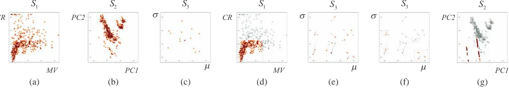
Fig. 1. An illustrative example for a joint visual analysis of items and dimensions of the “Boston Housing Prices” dataset. Three scatterplots are set up first: a)S1: house prices (MV) vs. crime rate (CR), b)S2: the first two principal components (PC1vs.PC2), c)S3: mean (µ) vs. standard deviation
(σ) values for all the dimensions of the data. d) The main trend in the data is selected inS1. e)µandσvalues are re-computed for the selected
items and changes are visualized inS3. f) Dimensions that deviate less are selected for a re-computation of the PCA. g) PCA results (before and
after) are visualized in a F+C style.
or not, while kurt indicates the peakedness of a distribution and IQR is a robust statistics that also describes the variance of a distribution.
3 ANILLUSTRATIVEDUALANALYSISEXAMPLE
Before we present our more formal model further below, we first de-scribe an illustrative example where a visual analysis of data items is carried out together with a visual analysis of the dimensions. Our aim here is not to already provide a comprehensive guide, but to informally demonstrate the basics of our dual analysis model.
As also generally in this paper, we assume that our datasets come in a tabular form with n items (rows) xj∈Ω(set of items), each of which with values in m dimensions (columns) dk∈∆(set of dimen-sions). In the following, we denote the kth value of the jth item as
xj,k. For this first illustration, we study the well-known ‘Boston
Neigh-borhood Housing Prices’ dataset [16]. This dataset contains informa-tion gathered by the U.S Census Service to understand the relainforma-tion between housing prices and other factors in the area of Boston, Mas-sachusetts. It consists of 506 samples xj and 14 dimensions dk(i.e., |Ω|=506,|∆|=14). Some of the dimensions that we refer to later are: ‘median value of owner-occupied homes’ (MV),‘crime rate by town’ (CR), ‘proportion of houses built before 1940’ (AG) and ‘proportion of lower status of the population’ (LS).
In our analysis, we utilize PCA to understand the intrinsic dimen-sionality of this dataset. To reduce the effects of outliers on PCA, we analyze the data to determine outlier-free dimensions. We compare PCA results based on all dimensions and those computed for only se-lected dimensions, in order to achieve a better interpretation of the analysis results.
To enable the comparability of dimensions, the analysis starts with a normalization of the dimensions. To normalize the dimensions, we ap-ply linear scaling to the unit interval in this case. We then estimate the mean (µ) and standard deviation (σ) of all the columns (dimensions), in order to get a first impression of the included data distributions. We apply PCA to all the dimensions and project the data onto the first two principal components (PC1, PC2). We continue with the visualization of the items in a scatterplot S1(Figure 1-a) with axes CR and MV and
another scatterplot S2(Figure 1-b) with axes PC1 and PC2.
Addition-ally, we plot theµandσvalues of all dimensions in a scatterplot S3
(Figure 1-c).
We then start the interactive analysis by brushing (selecting) a sub-set of items in S1. This brush leaves out the larger values of MV and
CR and selects the items which (roughly) amount to the main trend in the data (Figure 1-d). As a next step, theµandσ values are es-timated (automatically) for the selected items and sent to S3. As a
result, S3gets updated to show the dimensions’ statistics with respect
to both the items selection as well as with respect to all of the items (Figure 1-e). Theµandσvalues corresponding to the selected subset are highlighted (with orange color), while the originalµ andσ val-ues (corresponding to the entire dataset) are presented as reference (in gray). The two points in the scatterplot which correspond to the same dimension (entire dataset vs. selected subset) are connected with a
ta-pered line to ease their identification. In Figure 1-e, we see that while the values for some of the dimensions changed prominently, some of them are not much affected by the selection. A simple first interpre-tation of the resulting visualization is that the dimensions that did not deviate so much due to the selection, possibly can be considered to be less sensitive to non-standard values of MV and CR. We then select the most “stable” dimensions in S3and PCA is applied automatically
using only the dimensions selected in Figure 1-f. We then project all the items to the newly computed principal components and send the resulting values to S2. Through a focus+context visualization of the
two different projections of the items in S2, we can clearly see that the
projection results changed dramatically (Figure 1-g). An interesting split into two groups with respect to the new PC1, for example, can be observed. In such an explorative setting, the analysis may not always converge to the mathematically best-possible result. However, through the selection of suitable statistics and the use of interactive brushing, the analysis leads to both additional insight on the data and results that are easier to interpret. Guidelines for a robust analysis process are provided in Section 6.
The above presented short illustration brings up new opportunities for the analysis of high-dimensional data. Such a dual visual analysis of both items and dimensions leads to a novel perspective on looking at high-dimensional data. In the following section, we formalize this dual analysis idea in the form of a model by defining the underlying linking&brushing and focus+context (F+C) visualization mechanisms.
4 THEDUALANALYSISMODEL
Analysts are often faced with high-dimensional data which comes in a tabular form where items are rows and dimensions are columns. In conventional visual analysis approaches that involve multiple coor-dinated views, items are visualized using visualizations like scatter-plots, histograms or parallel coordinates. In such visualizations, the items are plotted in the views as opposed to the dimensions of the data. The visual analysis of data items is often carried out using link-ing&brushing and focus+context visualization. Our dual visual analy-sis concept builds upon these conventional practices and proposes the visual analysis of data in two linked spaces, namely in items space I, and in dimensions space D. With items space we refer to a visual-ization domain where each visual entity in a visualvisual-ization corresponds to a data item. In the dimensions space, however, each visual entity represents a dimension of the data. To illustrate, if we visualize the housing data in both of the spaces, using scatterplots, a point in items space corresponds to a single house, whereas in the dimensions space, a single point represents a dimension, crime rate by town, for instance. By separating the visual analysis space into two, we provide opportu-nities for the joint and parallel analysis of items and dimensions.
MVA Results
Data Item
Data Dimension
Dimension Statistics Item
Selection
Dimension Selection Items
Space
[image:5.595.346.520.47.284.2]Dimensions Space
Fig. 2. The dual analysis model sketched. Visual analysis is per-formed over two spaces, items space and dimensions space. Visual entities correspond to items in items space and dimensions in dimen-sions space. Analysis advances iteratively by selecting items and di-mensions. The interactions enable the joint and linked exploration of dimension statistics and multivariate analysis (MVA) results.
model is achieved by linking the visualizations in the two spaces. In order to fully accomplish this link, we formulate brushing and
focus+context visualization mechanisms, as well as transformations
which are needed to establish the relation between the two spaces.
4.1 Data Transformations
The iterative analysis of items and dimensions is at the core of our model. During a typical iteration, the focus of the analysis moves from one space to the other. In order to achieve the transitions be-tween items and dimensions space, our model requires a set of data transformations.
From dimensions space D to items space I: The basis for the
first type of transformations relates to the MVA methods that oper-ate on the dimensions∆. Such methods are here denoted by f . We generalize transformations f to operations that create l new data di-mensions when applied. In the illustrative example in Section 3, PCA is an example of such an f transformation. Throughout the iterative analysis loop, the ithtransformation of data through f is defined as:
TDi(f):∆′→f ∆iwhere∆i={d
c+1, ...,dc+l}with any da being a full
new column da={x1,a, ...,xn,a}
Tand c=∑i−1
t=0|∆t|. Note that, in these
transformations, all the items are projected onto the new dimensions and∆′⊆∆represents a selection of dimensions of the data before the transformation. At a certain point in the iterative loop, where the ana-lyst have made y of these transformations, the final set of dimensions is denoted as∆+={∆0
, ...,∆
y}with∆0=∆, i.e., the original data
dimensions.
Although we exemplify PCA as one f method, it can also be any other MVA tool which creates a mapping of the original dimensions. It is possible to consider methods like multidimensional scaling (MDS) and factor analysis (which are other dimension reduction techniques), clustering (which maps the data items to class labels), and LDA (which maps the data items to known classes) [20].
As an initial transformation, which usually precedes the statistical analysis as well as the visualization, we normalize the dataset so that values in all the dimensions are quantitative and comparable. Normal-ization also ensures that all of our dimensions are suitable for visu-alization in a scatterplot, histogram, etc. Moreover, normvisu-alization is an essential step for most of the multivariate analysis processes [27]. This normalization step is denoted with TD1(N)where N is a normal-ization method, such as linear normalnormal-ization to the unit interval or z-standardization [27]. The results of TD1(N)is denoted with∆1where
∆1
=|∆|.
From I to D: We use transformations s to iterate from items space
to dimensions space. Examples of s can be descriptive statistics or an
CR
MV
s
m
PC2
PC1
CR
MV
s
m
s
m
s'
m'
PC1' PC2'
PC1 PC2
Brush Items: 3.BI:W®W'
5.BD:D®D' 6.TDi:D'®Di
4.TIr:W'®Wr Items
Space
Dimensions Space
Initial Setup
Iterative Analysis 1 1
.TD(PCA)
Update MVA Results:
Brush Dimensions:
Update Statistics:
[image:5.595.72.271.48.194.2]2.T1( , ) I s m
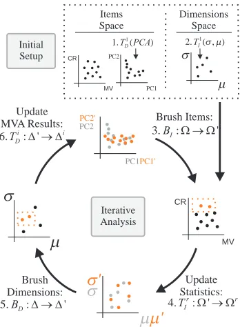
Fig. 3. Items space views both visualize normalized dimensions, e.g., CR or MV in housing data, and derived dimensions, e.g., PCA results
PC1orPC2. Dimensions space views visualize dimensions as opposed to statistics, such asµorσ. Here, the initial setup is done by computing
PCs (1),µ andσ (2). Brushes from items space (3) triggers F+C vi-sualizations in dimensions space by going through transformations (4). Similarly, brushes from dimensions space (5) updates the MVA result vi-sualization through transformations (6). This interactive loop continues iteratively by modifying the selections on both sides.
aggregation of data items. Here, we mainly consider statistics as s. If we considerσas s, the result of the transformation are theσvalues for each and every dimension in the data. In the rthiteration of the analysis the transformation which computes g new values per dimension using
s is defined as: Tr I(s):Ω′
s
→ΩrwhereΩr={x
e+1, ...,xe+g}with any
xabeing a full new row xa={xa,1, ...,xa,m}and e=∑
r−1
t=0|Ωt|. Here, Ω′⊆Ωrepresents a selection of items. In the course of the analysis,
the analyst can make z of these transformations where she produces the final set of computed valuesΩ+={Ω0
, ...,Ω
z}. To generalize,
regarding the set of possible s functions or statistics, it is possible to consider descriptive statistics such as mean, variance, skewness, kur-tosis and more elaborate values like statistical test results or robust estimates.
The selection of dimensions∆′and itemsΩ′is formulated through a degree-of-interest (doi) mechanism. Similar to fuzzy set definitions, we define ∆′= (∆,doi∆)andΩ
′= (Ω
,doiΩ)where doi∆ and doiΩ
are mappings to define selection degrees. In the case of binary se-lections, where an item is either selected or not, selections are de-fined as doiΩ:Ω→ {0,1}. In the case of continuous doi values,
where items are selected to a certain degree, selections are defined as doiΩ:Ω→[0,1]. Such a continuous selection mechanism can be
achieved through smooth brushes [5]. The addition of smooth brushes brings the possibility of weighing the dimensions prior to a dimension reduction operation, for instance.
4.2 Brushing & Focus+Context Visualization
s
m
PC2
PC1
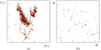
[image:6.595.317.567.48.149.2](a) (b)
Fig. 4. Focus+context visualizations in scatterplots of two different PCA results (a) and of two sets of statisticsσ,µ(b). The recomputed values are in focus after the selection, and the values from before the selection are provided as context. Depending on the point count, two different styles are employed (with and without lines).
It is worthwhile to mention that the columns of our dataset are treated as rows in dimensions space. Accordingly, our approach can also be thought of as transposing the dataset and performing the visual analy-sis using a different perspective in dimensions space. In the illustrative example in Section 3, S1and S2are examples of VIand S3is an
exam-ple of VD.
We follow the conventional linking&brushing mechanism between the views that are in the same space; i.e., when certain items in a VI are brushed, the same items are highlighted in other VIs using a fo-cus+context visualization and the same mechanism works also for VDs. In order to define the links between views from different spaces, we extend this mechanism by handling the brushes through the f and s transformations. The transitions between the two spaces and illustra-tions for the associated F+C visualizaillustra-tions scheme are illustrated in Figure 3.
A brush in VIis defined as BI:Ω→Ω ′
whereΩ′⊆Ω. In order to transfer BIto dimensions space, brushed itemsΩ
′
are transformed by
TI(s)rusing the current s. The resulting valuesΩ+update visualiza-tions in dimensions space. An example of such a brushing operation can be seen in Figure 1-d,e. Here,σandµvalues (i.e., s transforma-tions) are re-computed for the selected items in S1and the
computa-tions update S3.
A brush in VDis defined as BD:∆→∆ ′
with∆′⊆∆. BDis trans-ferred to items space by going through the transformation TD(f)i. And, the resulting∆′ update VIs accordingly. An example for this type of operation can be seen in Figure 1-f,g. Here, the dimensions are selected in S3and the selection of dimensions is an input to the PCA
operation.
In a typical F+C visualization, the common interpretation of focus are the selected items and the context is the rest. In our model, we slightly extend this definition of F+C visualization. Focus and context are two different visualizations of the same items, that are computed using different subsets of the dataset. The results of the last transfor-mation ( f or s) is set as the focus and those of the preceding one as the context. Notice that each point in a scatterplot is drawn twice, once with the old and once with the new value. Here, we follow a simple strategy to show the results. If the point count is large, we plot fo-cus and context in different colors (Figure 4-a). If the point count is small, we additionally connect the related points with a tapered line (Figure 4-b). Although this simple solution is adequate for illustrative purposes in this paper, one should think of more intelligent ways to achieve comparative visualizations, e.g., difference views [24].
One important point to mention, also, is that, in the F+C visual-izations of the first type of views, the focus is computed as a “lazy evaluation”, i.e., the focus of a view, is linked to a brush and it is com-puted automatically as the brush moves. This approach is necessary for the sake of interactivity in the model. Additionally, the context of the views can be updated at any point throughout the analysis. With such an extension, it is possible to compare the statistics and analysis results of any different item-dimension subsets.
[image:6.595.93.269.50.138.2](a) (b)
Fig. 5. The proposed dual analysis extended to parallel coordinates plots (PCP). a) PCP from items space visualizing items over the first three principal components. b) PCP from dimensions space visualizing
σ,kurt,skewandIQRvalues for the dimensions.
4.3 Extensions to the Model
It is possible to extend the proposed dual analysis method to also in-corporate different visualization techniques, e.g., parallel coordinates plots (PCP). While lines in a PCP represent data items in items space, they represent dimensions in dimensions space. Accordingly, axes of a PCP in items space are the original dimensions of the dataset and they correspond to differentΩ+in dimensions space. An example of these dual PCPs can be seen in Figure 5. In order to visualize the deviations and employ our dual focus+context approach in a PCP, comparative visualization methods, like Temporal Parallel Coordinates [19] can be utilized. Another possible extension is to employ glyphs as the visual entities in dimensions space [37]. One can think of glyphs where each visual channel represent differentΩ+values.
In its current state, the model is designed for datasets that come in a 2D tabular form. However, it is possible to extend the model to 3D data tables, e.g., to datasets where the third dimension is time. In the dual analysis of such datasets, visualizations in items space are con-ventional visualizations of temporal data, i.e., each data item is repre-sented by a curve over time in a function plot. In dimensions space, however, each curve represents a dimension over time. We perform s transformations on each temporal dimension and visualize the results in a function plot in dimensions space. In Figure 6, this mechanism is illustrated. Here, we visualize measurements from a weather station in Bergen, Norway. The dataset contains daily measurements, such as temperature, pressure, precipitation, for all the years between 2000 and 2010. In Figure 6-a, each curve represents the temperature values for one year. On the other side, in dimensions space, we computeσ values for each dimension over time. And the result is a curve for each dimension plotted againstσvalues as seen in Figure 6-b.
5 PROTOTYPEIMPLEMENTATION OF THEMODEL
We implemented our model in an interactive visual analysis environ-ment where we enable linking&brushing and focus+context
visualiza-(a) (b)
Temporal Data Item
Temp
Time Time
s
Temporal Data Dimension
[image:6.595.318.564.582.676.2]Table 1. Possible multivariate statistical tools (f transformations) and corresponding statisticssfor the dual analysis setting
Analysis f s
Dimension reduction (unsupervised)
PCA, MDS loadings, mean, variance, me-dian, skewness, kurtosis, IQR
Dimension reduction (supervised)
LDA, SVM variance, information theory
Finding groups in data Clustering mean, variance, median, IQR
tions of data in scatterplots and other views. We implemented two types of scatterplots, with two types of F+C visualization, as already discussed above. Our aim with the prototype implementation is to showcase the utilization of the system using simple visualization solu-tions.
Our implementation utilizes composite brushing, as proposed by Allen and Ward [25], as the underlying brushing mechanism. In this mechanism, each brush is combined with existing brushes by a Boolean operator op with op∈ {∪,∩,¬}, where ∪represents the
union,∩represents the intersection and¬represents the not operator. To ensure an easier utilization of different types of views, the visual-ization space is physically divided into two, one to show items space and the other one for dimensions space. Additionally, to include a wider range of MVA tools into the system, we integrate the R statisti-cal computation package into our system [32].
6 DUALANALYSISPROCEDURES
The dual analysis process provides a number of opportunities in the visual analysis of high-dimensional data. Here, we provide a guide for selecting and using the transformations and visualizations in the proposed dual setting.
6.1 Selecting Transformations
Depending on the type and the goal of the analysis, the analyst deter-mines the multivariate statistical analysis tools and statistics to utilize. The selected tools and statistics then correspond to the transformations in our model. In Table 1 we provide a non-exhaustive list of common MVA tools f and statistics s that are suitable for the dual analysis scheme. Note that the dual analysis model is not specific to any of these methods.
One important type of f transformations are unsupervised dimen-sion reduction methods such as PCA and MDS. The reliability of the results of such methods depend on the normality and “outlier-freeness” of the data columns. Additionally, to improve the interpretability of the results, redundant dimensions should be discarded. Principle com-ponent loadings,σ and the interquartile range (IQR) can be used to assess the dimensions’ redundancy whileµ,σ, skewness and kurtosis can be used to evaluate normality and the existence of outliers. Similar
s transformations are preferred for clustering, where the quality of the
results is affected by a high number of dimensions as well as outliers in the data.
In supervised dimension reduction methods like LDA and Support Vector Machines (SVM), the normality of the data is not required. However, the selection of dimensions is crucial with respect to the quality of the results, also. In order to determine important dimen-sions,σ, IQR or information theoretic measures can be utilized [15].
In all of these methods, filtering dimensions prior to the analysis both improves the quality and interpretability of the results. Therefore, dimensions need to be evaluated in terms of their variance (saliency) and/or entropy [15]. Dimensions that are poor in information content, i.e., with a low variance, low entropy, near-zero loadings in PCs, can be marked as “redundant” and left out from the analysis.
6.2 The Analysis Process
In the following, we provide a task-based guideline to carry out an analysis in the proposed dual framework:
• To understand the relations between dimensions: A subset of items
are selected first. As a result, the changes in s values in dimensions space reveal the correlation between dimensions with respect to the selections. Larger deviations in s values indicate a higher correla-tion.
• To explore the dimensions that determine the main trend or the
out-liers in the data: Items that correspond to the main trend or outout-liers are selected in a lower-dimensional projection of the data. Devia-tions in dimensions space reveal such dimensions.
• To leave out/select dimensions: Dimensions are evaluated in terms
of the information they contain through the use of certain s such as σ, principal component loadings and entropy.
We follow these guidelines and go through the steps of a detailed anal-ysis process that is similar to the one we presented earlier in Section 3. In this analysis, we aim to explore the relation between dimensions and find lower-dimensional representations of the data to derive new hypotheses. Hence, we set PCA to be our main f andσ,µ, skew, and,
kurt to be s transformations.
The analysis starts with the normalization step (TD1), where the data is scaled, for example, to the unit interval and followed by the com-putation ofσ,µ, kurt and skew values for all the dimensions using all the items. Additionally, we perform PCA on the data using all the dimensions.
In the next part of the analysis, we try to understand the relations between dimensions. The changes in basic descriptive statistics (such asµandσ) due to brushes in items space are easy to interpret and pro-vide information on the correlations between dimensions. Therefore in this step, we chooseµ andσ as the visualization axes in dimen-sions space. We visualize the items in a scatterplot with axes CR vs. AG (VI0) and dimensions in a scatterplot ofµvs.σ(VD0).
We select the areas with old houses in VI0in Figure 7-a. In dimen-sions space (in VD0), we observe howσandµvalues deviate after the brushing operation. Here, we see thatσvalues for LS dropped signif-icantly, this is due to the fact that the selection of high AG values is sampling the lower population (LS) dimension unevenly. We interpret this observation as follows:
High values of AG are related to very low values of LS, while low AG values lead to a much broader range of values for LS. In other words, only a very low proportion of the lower status of the population is living in areas with old houses. When focusing on areas with a lower proportion of old houses, there is no limitation with respect to the proportion of the lower status population. This “change point” in the relation between AG and LS was thus discovered by the big deviation ofµandσ when using all or just the selected data. On the contrary, we see that there is almost no change in theµandσvalues on the dimension MV, indicating about the same behavior of the selected and the original data points.
In order to verify these impressions, we visualize the AG dimension as opposed to both LS and MV (VI1, VI2). We see in VI2in figure 7-a that in areas with old houses, the proportion of lower society is also very low. In VI1, we see that MV values vary over a wide range of values for the selected houses (i.e., in areas with older houses). Therefore, it is not possible to talk about a correlation between MV and AG.
The second phase of the analysis involves the elimination of outliers to refine the PCA results. To determine outliers, we use the PCA re-sults (which are already biased by the outliers) that are obtained earlier (VI3). VI4in Figure 7-b shows how PCA results change after removing the outliers with the brush in VI3. The updated PCA results now dis-play two groups of items, however there is still substantial variation in the groups.
(a) (b) Select areas
with high AG
AG CR
V
I0:
s
m
V
D0:
V
D0:
AG MV
V
I1:
AG LS
V
I2:
PC2
PC1
V
I3:
PC2'
PC1'
V
I4:
PC2'
PC1'
V
I4:
V
I4:
skewV
D1:
V
D0:
Less Variance{
}
More VarianceLeave out
Outliers Select dimensionswith and ~ 0
kurt skew
Select items in the group
1
3
2
4
s
V
D0:
m
Source of outliers
kurt
PC2'
PC1'
Two main groups
s
m
[image:8.595.65.568.49.271.2]Distinctive dimensions
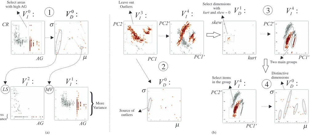
Fig. 7. A dual analysis of the housing dataset. a) Houses in areas that have a large proportion of old houses (high AG values) are selected inV0 I. VD0is updated using newµandσvalues (1). Deviations inVD0indicate a correlation between dimensions w.r.t. the selection. The most deviating (LS) and the least deviating (MV) dimensions are plotted for a deeper analysis. The variance of the selections (inV1
I andVI2) justifies the deviations inV0
D. b) Outliers are removed inVI3and PCA is applied with the selected items.VI4is updated with the new results (2). As a result of the selection inV3
I, one of the dimensions is marked inVD0as the source of the outliers. Before operation (3), the current PCA results are set as the context of V4
I. Normally distributed dimensions, w.r.t. kurtandskewvalues inVD1, are selected (3). Updated PCA results now display two groups. One of the groups is selected inVI4andVD0now reveals the dimensions that distinguish the selected group.
σvalues for the Tax-rate (TAX) dimension changed significantly. We mark the TAX dimension as the source of these outliers and remove this dimension (with a¬brush which is not shown in the image) from the analysis before we move on to the next step. As an intermediate operation, we set the current PCA results (obtained by removing the outliers) as the context of our new visualization (VI4).
We would now like to evaluate the dimensions’ normality to decide whether to include them in the analysis. Therefore, we continue the analysis in dimensions space. Since kurt and skew values are indica-tors of normality, i.e., both the skewness and kurtosis for normal distri-bution are 0, we select dimensions through the kurt vs. skew plot (VD1). We select dimensions (marked with 3 in the figure) which are more likely to follow a normal distribution by selecting dimensions with values around 0. The updated PCA plot displays two well-separated groups that have less variance throughout the group.
We perform a final brush in VI4to understand which of the dimen-sions are more distinctive for these groups (Figure 7-b, 4). We se-lect the larger group on the left and observe the changes inµvs.σ values. Here, we discover four dimensions: “nitric oxides concentra-tion”, “number of rooms”, “pupil-teacher ratio”, “proportion of black by town” to be the distinctive dimensions. These dimensions can now be used for further analysis, e.g., in clustering the houses.
The proposed dual analysis method continues iteratively with inter-actions between the two spaces. Since the analyst gets an immediate feedback of the interactions, item and dimension selections are refined iteratively until the analyst is satisfied with the results. Note that, the above analysis presents the interpretations of a set of specific statistics and statistical tools. The interpretations of the views and interactions needs to be formulated on the nature of the problem and statistics used.
7 USECASE: MOLECULARCLASSIFICATION USINGDNA MI
-CROARRAYS
DNA microarrays and high-density oligonucleotide chips are impor-tant monitoring technologies used in cancer research [6]. This mon-itoring is applied to different tissue samples which are known to be taken from a specific type of tumor. The resulting dataset then
con-tains the expression levels of thousands of genes for these different samples. In molecular level cancer research, these datasets are ana-lyzed to distinguish between cancer classes or even to discover new types of cancers. Two of the main goals in this research which in-volves statistical approaches are: classifying the samples into classes of tumors and identifying important genes which plays a role in this classification [6]. The statistical analysis of such data has always been a challenge as the dataset contains a very large number of genes (di-mensions) compared to the number of tissue samples (items). As the analysts are interested in identifying both the groups of genes and the groups of samples, in the analysis of microarray data, one has to ana-lyze both the original and the transposed version of the dataset.
In this use-case, we work on a gene expression dataset provided by Golub et al. [12]. Here, the samples are known to come from two types of acute leukemia, namely acute lymphoblastic leukemia (ALL) and acute myeloid leukemia (AML). The dataset consists of 7129 genes taken from 38 different tissue samples where 27 are known to be ALL and the rest AML. We treat the dataset in the form that, genes are items (Ω) and samples are dimensions (∆) as it is the standard way in statistical analysis of microarray data [9].
The task in this use-case is to find a good classifier that distinguish the tissue samples into ALL and AML types. In order perform the classification, we use LDA as an integrated MVA tool. Our aim is to select a number of genes that are more important in the classification of the tissues and thus, improve the performance of the classifier. Without any modification, i.e., using all the samples and all the genes, LDA is able to classify 29 of the 38 samples correctly.
In DNA microarray data analysis, outlier genes are of more impor-tance in the classification of the tissues [9]. Therefore, we focus the analysis on selecting the genes. We, firstly, plot the genes in a scatter-plot using PCA and secondly, select outlier genes from the scatter-plot to per-form the classification with the selected genes. We utilize our model to achieve more reliable PCA results, thus improving the classification performance.
“im-PC2
PC1
Outlier genes
m
s
PC2
PC1 PC1
PC2
PCA of genes
Tissue Loadings
Tissue Statistics
PCA of genes
Tissue Loadings
PCA of genes
PCA of genes
ll_1 ll_2
ll_1 ll_2
PC2
PC1 IQR
s
Tissue Statistics
(a) (b)
(c) (d)
(e) (f)
(g) (h)
Outlier genes Outlier
tissue
Fig. 8. An analysis of microarray data. The task is to select a small number of genes (preferably outliers) for the discrimination of tissues. a) PCA is applied on the genes. There is a large variation and a large number of outliers. b) Tissues are plotted against their PCA loadingslls for PC1 and PC2, where zero loadings indicate redundancy. c) Tissues with large loadings are selected. d) Less number of outlier genes due to the new PCA results. e) Tissues are visualized in aσvs.IQRplot for the selection of tissues with a smaller number of outliers. f) PCA is computed using the selected tissues. g-h) Analyzing the properties of tissues w.r.t. the genes. For a selected group of genes, an outlier tissue is discovered.
portant” genes and filter out the less interesting ones (Figure 8-a). We visualize the tissues in dimensions space and update PCA results by selecting the tissues (dimensions in this case). To visualize the tissues, we utilize the loadings ll of the PCs as our s function. The loadings are the weights of each single tissue (dimension) in the resulting PCs and they indicate how much a tissue contributes to the principal com-ponent. In Figure 8-b, tissues are plotted against ll values (for PC1 and PC2). Here, the ones with higher loadings (in absolute values) are more important variables and the ones with close-to-zero loadings are considered as redundant. We leave out redundant samples (Figure 8-c) and visualize the updated PCA results (Figure 8-d). Here, we see that, we get a smaller number of outlier genes. We select the outlier genes and apply LDA using only these genes. We observe that with this setting, LDA is able classify 30 samples correctly.
We continue the analysis by visualizing the tissues in a interquartile-range (IQR) vs.σscatterplot. Bothσand IQR are mea-sures of variability, howeverσ is easily affected by outliers. As a result, if there is a large deviation between IQR andσ values of a di-mension, this dimension is likely to contain outliers. In Figure 8-e, we remove such dimensions and re-compute PCA with the selected dimensions. As a result, we observe that we get a more reliable PCA result (Figure 8-f). By selecting the outliers, we observe that LDA classified 34 samples correctly. Additionally, we select a group of out-lier genes (Figure 8-g) to explore how the tissues relate to this selected group. In Figure 8-h, we see that while theµandσvalues for most of the tissues change in a similar manner, one tissue is clearly an outlier. In this use-case, we demonstrate how our model brings new possi-bilities to the analysis of DNA microarrays. Additionally, we demon-strate how a statistical tool LDA, is used as a validation step. At each iteration, LDA results provides an immediate feedback if the current selection improved the results or not.
8 CONCLUSION
In this paper, we introduce a visual analysis model that enables the dual analysis of items and dimensions of high-dimensional data. The iterative and joint analysis of the data is performed over two linked
spaces: items space and dimensions space. The analysis iterates through the interaction with the items in items space and with the di-mensions in didi-mensions space. In our model, didi-mensions are the basic visual entities of the visual analysis in dimensions space. Such an ap-proach enables us to extend the knowledge in the interactive visual analysis of data items to the visual analysis of dimensions. To the best of our knowledge, our model is one of the first IVA approaches, where the dimensions are interactively and iteratively analyzed as first-order visual entities together with the actual data items.
We present a formal definition of our model by defining: i) the data transformations that are used to iterate from one space to the other; ii) brushing and F+C visualization to achieve the linking of views. We define how MVA tools and statistics are tightly integrated into the dual analysis concept. Additionally, we present a set of possible analysis procedures that involve the joint interaction of items and dimensions. Finally, we evaluate the model in the context of a DNA microarray data analysis, where the analysis of data items and dimensions is equally important.
are improved.
In this paper, we do not focus on specific MVA tools or specific statistics. Therefore, we picked some of the well-known tools and statistics such as PCA, LDA,µ,σ, skew, kurt, and IQR. The concept of dual analysis can have utilizations with different MVA tools. We plan to work on visualizations and advanced interaction mechanisms that are more specific to certain MVA tools. We will further investigate the utilization of our model in the context of other application domains where the dual analysis concept could prove to be helpful.
As a future work, we will extend our model to include statistics that consider pairs of dimensions, e.g., correlation, regression. Addition-ally, as another extension, we plan to include visualizations that can provide a formal validation for the interactions, e.g., projection preci-sion [28].
We think that the presented model brings up new opportunities in the analysis of high-dimensional data. By looking at the data from two different perspectives with the help of MVA tools, it is possible to build elaborate and specialized visual analysis frameworks.
ACKNOWLEDGMENTS
The authors wish to thank Animesh Sharma for providing informa-tion and data on DNA microarrays. The authors also thank Johannes Kehrer and J´ulius Parulek for the valuable discussions and comments.
REFERENCES
[1] R. Agrawal, J. Gehrke, D. Gunopulos, and P. Raghavan. Automatic sub-space clustering of high dimensional data for data mining applications. In Proceedings of the 1998 ACM SIGMOD international conference on Management of data, pages 94–105. ACM, 1998.
[2] G. Andrienko, N. Andrienko, S. Bremm, T. Schreck, T. Von Landes-berger, P. Bak, and D. Keim. Space-in-time and time-in-space self-organizing maps for exploring spatiotemporal patterns. In Computer Graphics Forum, volume 29, pages 913–922. Wiley Online Library, 2010. [3] W. Berger, H. Piringer, P. Filzmoser, and E. Gr¨oller. Uncertainty-aware exploration of continuous parameter spaces using multivariate prediction. Computer Graphics Forum, 30(3):911–920, 2011.
[4] C. D. Correa, Y.-H. Chan, and K.-L. Ma. A framework for uncertainty-aware visual analytics. In Proc. IEEE Symposium on Visual Analytics Science and Technology VAST 2009, pages 51–58, 2009.
[5] H. Doleisch, M. Gasser, and H. Hauser. Interactive feature specification for focus+context visualization of complex simulation data. In Proceed-ings of the symposium on Data visualisation 2003, VISSYM ’03, pages 239–248. Eurographics Association, 2003.
[6] S. Dudoit, J. Fridlyand, and T. Speed. Comparison of discrimination methods for the classification of tumors using gene expression data. Jour-nal of the American statistical association, 97(457):77–87, 2002. [7] A. Farcomeni. An exact approach to sparse principal component analysis.
Computational Statistics, 24(4):583–604, 2009.
[8] P. Filzmoser, K. Hron, and C. Reimann. Principal component analysis for compositional data with outliers. Environmetrics, 20(6):621–632, 2009. [9] P. Filzmoser, R. Maronna, and M. Werner. Outlier identification in high
dimensions. Computational Statistics & Data Analysis, 52(3):1694– 1711, 2008.
[10] R. Fuchs and H. Hauser. Visualization of multi-variate scientific data. Computer Graphics Forum, 28(6):1670–1690, 2009.
[11] R. Fuchs, J. Waser, and M. E. Gr¨oller. Visual human+machine learning. IEEE TVCG, 15(6):1327–1334, Oct. 2009.
[12] T. Golub, D. Slonim, P. Tamayo, C. Huard, M. Gaasenbeek, J. Mesirov, H. Coller, M. Loh, J. Downing, M. Caligiuri, et al. Molecular classifi-cation of cancer: class discovery and class prediction by gene expression monitoring. Science, 286(5439):531, 1999.
[13] L. J. Gosink, C. Garth, J. C. Anderson, E. W. Bethel, and K. I. Joy. An application of multivariate statistical analysis for query-driven visu-alization. IEEE Transactions on Visualization and Computer Graphics, 17:264–275, 2011.
[14] Z. Guo, M. O. Ward, and E. A. Rundensteiner. Model space visualiza-tion for multivariate linear trend discovery. In Proc. IEEE Symp. Visual Analytics Science and Technology VAST 2009, pages 75–82, 2009. [15] I. Guyon and A. Elisseeff. An introduction to variable and feature
selec-tion. The Journal of Machine Learning Research, 3:1157–1182, 2003.
[16] D. Harrison et al. Hedonic housing prices and the demand for clean air. Journal of Environmental Economics and Management, 5(1):81–102, 1978.
[17] H. J¨anicke, M. B¨ottinger, and G. Scheuermann. Brushing of attribute clouds for the visualization of multivariate data. — IEEE Transactions on Visualization and Computer Graphics, pages 1459–1466, 2008. [18] D. H. Jeong, C. Ziemkiewicz, B. Fisher, W. Ribarsky, and R. Chang. ipca:
An interactive system for pca-based visual analytics. Computer Graphics Forum, 28:767–774(8), 2009.
[19] J. Johansson, P. Ljung, and M. Cooper. Depth cues and density in tempo-ral patempo-rallel coordinates. In EuroVis, pages 35–42, 2007.
[20] R. Johnson and D. Wichern. Applied multivariate statistical analysis, volume 6. Prentice Hall Upper Saddle River, NJ:, 2007.
[21] B. K´egl. Intrinsic dimension estimation using packing numbers. Ad-vances in Neural Information Processing Systems, pages 697–704, 2003. [22] J. Kehrer, P. Filzmoser, and H. Hauser. Brushing moments in interactive
visual analysis. Computer Graphics Forum, 29(3):813–822, 2010. [23] D. Keim, F. Mansmann, J. Schneidewind, J. Thomas, and H. Ziegler.
Vi-sual analytics: Scope and challenges. ViVi-sual Data Mining, pages 76–90, 2008.
[24] O. D. Lampe, J. Kehrer, and H. Hauser. Visual analysis of multivari-ate movement data using interactive difference views. In Proceedings of Vision, Modeling, and Visualization (VMV 2010), pages 315–322, 2010. [25] A. R. Martin and M. O. Ward. High dimensional brushing for
interac-tive exploration of multivariate data. In VIS ’95: Proceedings of the 6th conference on Visualization ’95, page 271, Washington, DC, USA, 1995. IEEE Computer Society.
[26] K. Matkovic, W. Freiler, D. Gracanin, and H. Hauser. Comvis: A coor-dinated multiple views system for prototyping new visualization technol-ogy. Information Visualisation, International Conference on, 0:215–220, 2008.
[27] D. Pyle. Data preparation for data mining. Morgan Kaufmann, 1999. [28] T. Schreck, T. von Landesberger, and S. Bremm. Techniques for
precision-based visual analysis of projected data. Information Visual-ization, 9(3):181–193, 2010.
[29] J. Seo and B. Shneiderman. A rank-by-feature framework for unsuper-vised multidimensional data exploration using low dimensional projec-tions. In Proc. IEEE Symposium on Information Visualization INFOVIS 2004, pages 65–72, 2004.
[30] B. Shneiderman. The eyes have it: a task by data type taxonomy for in-formation visualizations. In Visual Languages, 1996. Proceedings., IEEE Symposium on, pages 336 –343, Sept. 1996.
[31] C. Stolte, D. Tang, and P. Hanrahan. Polaris: a system for query, analysis, and visualization of multidimensional relational databases. IEEE Trans-actions on Visualization and Computer Graphics, 8(1):52–65, 2002. [32] R. D. C. Team. R: A Language and Environment for Statistical
Comput-ing. R Foundation for Statistical Computing, 2009.
[33] M. O. Ward. Xmdvtool: integrating multiple methods for visualizing multivariate data. In Proceedings of the conference on Visualization ’94, VIS ’94, pages 326–333. IEEE Computer Society Press, 1994. [34] C. Weaver. Cross-filtered views for multidimensional visual analysis.
IEEE Transactions on Visualization and Computer Graphics, 16:192– 204, March 2010.
[35] M. Williams and T. Munzner. Steerable, progressive multidimensional scaling. In Proceedings of the IEEE Symposium on Information Visu-alization, pages 57–64, Washington, DC, USA, 2004. IEEE Computer Society.
[36] P. Wong and R. Bergeron. 30 years of multidimensional multivariate visu-alization. In Proc. Workshop on Scientific Visualization, IEEE Computer Society Press, 1995.
[37] J. Yang, D. Hubball, M. Ward, E. Rundensteiner, and W. Ribarsky. Value and relation display: Interactive visual exploration of large data sets with hundreds of dimensions. Visualization and Computer Graphics, IEEE Transactions on, 13(3):494 –507, 2007.