Reversible jump Markov chain Monte Carlo method for parameter reduction in claims reserving

City, University of London Institutional Repository

Citation

:

This is the unspecified version of the paper.

This version of the publication may differ from the final published

version.

Permanent repository link:

Link to published version

:

Copyright and reuse:

City Research Online aims to make research

outputs of City, University of London available to a wider audience.

Copyright and Moral Rights remain with the author(s) and/or copyright

holders. URLs from City Research Online may be freely distributed and

linked to.

City Research Online: http://openaccess.city.ac.uk/ [email protected]

Reversible Jump Markov Chain Monte Carlo Method for

Parameter Reduction in Claims Reserving

Richard J. Verrall∗ Mario V. W¨uthrich†

Abstract

This paper presents an application of reversible jump Markov chain Monte Carlo (RJMCMC)

methods to the important problem of setting claims reserves in general insurance business.

These reserves are necessary because the premium is received early, but claims may take

years to be reported and settled. A measure of the uncertainty in these reserves estimates is

also needed for solvency purposes. The RJMCMC methods described in this paper represent

an improvement over the manual processes often employed in practice.

1

Introduction

The process of setting provisions for outstanding claims is an important part of the management

of general insurance companies. It is important that sufficient capital is held in order to pay

any emerging liabilities, but it is also important for the company not to over-reserve, in order

that the shareholders can benefit appropriately from the profits of the company. This process

requires skillful technical analysis, but it is also necessary to use sensible management judgment.

This analysis and judgment appropriately combined should result in claims reserves which are

sufficient for paying subsequent claims developments and which are relatively stable over time.

The setting of claims reserves usually begins with a technical method applied to data in a

straightforward way, followed by adjustments and fine-tuning in order to generate claims reserves

that are satisfactory in all senses. Often, the starting point is a simple method such as the

chain-ladder method, and one of the important aspects that then has to be further considered

are tail factors to estimate the future run-off of claims beyond the latest development year so

far observed. To be more specific, claims data is often studied in the form of a so-called claims

∗

Cass Business School, City University, 106 Bunhill Row, London EC1Y 8T2, UK

†

development triangle, where the rows of this triangle correspond to accident yearsi∈ {0, . . . , I}

and the columns correspond to development years j ∈ {0, . . . , I}. Claims observations at time

I are then collected in the upper claims development triangle

D_I ={Xi,j; i+j≤I, 1≤i≤I, 1≤j≤I}, (1.1)

and one aims to predict the lower triangle Dc

I = {Xi,j; i+j > I, 0≤i≤I, 0≤j≤I}. As

mentioned above, a common starting point is a model which specifies row parameters µi and

column parametersγj and then assumes a cross-classified model of the type

Eµi,γj [Xi,j] =µi γj, for all i, j∈ {0, . . . , I}. (1.2)

In practice this means that we need to estimate 2(I+ 1) parametersµ0, . . . , µI, γ0, . . . , γI from

(I + 1)(I+ 2)/2 observations Xi,j ∈ DI. For example, if we have I = 9 we need to estimate 20

parameters from 55 observations. In classical statistical theory, one would say that this model is

over-parametrized. The over-parametrization may lead to a good alignment of the parameters

to past observationsDI but therefore the predictive power for the lower triangle D_Icis quite low

because we have a large parameter uncertainty. The natural thing to do is to reduce the number

of parameters by fitting a parametric curve to (some of) the parameters: for example De

Jong-Zehnwirth [3] used a curve which is equivalent to assuming that the shape of the development

pattern γj is a gamma curve. Other papers have also investigated parametric curves to model

the development patternγj, but it is often found that in practice these curves are not sufficiently

flexible for most triangles of data. England-Verrall [4] suggested using generalized additive

mod-els, which apply local smoothing methods within the framework of the over-dispersed Poisson

model discussed below. However, the usual (manual) process used in practice is to try to find a

very simple model for the tail of the run-off, and use separate parameters for the early

develop-ment years. In this paper we suggest a method to replace this judgdevelop-mental process with a more

automatic mathematical procedure that should produce results which are at least as good as

those from the manual process. Bj¨orkwall et al. [1] have a very similar aim, but that paper uses

bootstrapping methods and we believe that the method presented in this paper has a number

of advantages. Thus, the aim is to model γ0, . . . , γk−1 individually up to a truncation index

k ∈ {1, . . . , I} and then fit an exponential decay to the remaining development parameters,

i.e. forj ∈ {k, . . . , I} we set

γj = exp{α−jβ},

for α ∈ _R and β ∈ _R+. It is this choice of the truncation index k which is often done rather

reserving model. This model will decide itself which the truncation index k is, only by doing

Bayesian inference from the dataD_I. That is, our Bayesian modeling framework will avoid any subjective choice of k but will only let the data speak. While we believe that there are some

parts of the process that require expert judgment, it is also our opinion that there are times

when the use of a manual procedure is inefficient and can, perhaps, give less reliable results.

Thus, we believe that it is helpful to consider replacing this part of the process with our more

automated method.

We study a whole family of models M_k, k ∈ {1, . . . , I}, all of which have a different number of parameters. We will let the data decide which model, Mk, it prefers (is the most likely

for the particular data set). This problem can be solved numerically with the reversible jump

Markov chain Monte Carlo (RJMCMC) method which is a particular Markov chain Monte Carlo

(MCMC) method that can jump between different models M_k that have different parameter sets. RJMCMC methods were developed by Green [9, 10], and these days we realize how powerful

they are for model selection purposes. Verrall et al. [15] also considered a Bayesian model for the

development pattern, using a different application of RJMCMC methods. Although, Verrall et

al. [15] presents an interesting model, which may well be of use in practice, the model presented

in this paper is much closer to the current actuarial practice. Having both of these methods

available should be of benefit to actuaries, and it is possible that either one of them will become

more widely used.

Organization of this paper. In Section 2 we introduce the Bayesian over-dispersed Poisson (ODP)

model. The crucial definition will be that we define a whole family of prior distributions for the

parameters. In Section 3 we describe in careful detail the RJMCMC method and its application

to our Bayesian ODP model. Finally, in Section 4 we provide examples and several remarks.

Moreover, we explain how the model is extended for tail factor estimation.

2

Bayesian over-dispersed Poisson model

In this section, we define the Bayesian ODP model which is used in this study. The classical ODP

model introduced by Renshaw-Verrall [14] and England-Verrall [5] is one of the most popular

stochastic claims reserving models. On the one hand it provides the chain-ladder reserves and on

the other hand it is very easy to generate bootstrap samples from. For the calculation of

often advantageous to introduce prior distributions for the parameters (including any available

expert knowledge on them), see Gisler-W¨uthrich [8] and B¨uhlmann et al. [2]. A Bayesian ODP

model was briefly covered in England-Verrall [5] and discussed in detail in England et al. [6].

The latter paper only considers cross-classified models with separate parameters for each

devel-opment year j, whereas we assume an exponential decay for the column parameters γj beyond

the truncation index,j∈ {k, . . . , I}. This leads to a whole family of modelsM_k,k∈ {1, . . . , I}, and Bayesian inference method will provide posterior probabilities for these models (from which

model selection can be done). This is set out formally in Model Assumptions 2.1.

Model Assumption 2.1 (Bayesian ODP model) Choose a fixedk∈ {1, . . . , I}. Then the

Bayesian ODP model M_k is given by the following model assumptions.

• Conditionally, given parameters ϑ = (µ0, . . . , µI, γ0, . . . , γI, ϕ), Xi,j are independent

ran-dom variables with

Xi,j

ϕ

ϑ

∼ Poi (µiγj/ϕ).

• Assume thatϕ >0 is a given constant and that the parameter vector

θk= (α, β, µ0, . . . , µI, γ0, . . . , γk−1) has prior distribution pk(θk) with independent components satisfying

µi ∼ Γ (s, s/mi) for i= 0, . . . , I,

γj ∼ Γ (v, v/cj) for j = 0, . . . , k−1,

α ∼ N(a, σ2), β ∼ N(b, τ2),

for given prior parameters mi, s, cj, v, σ, τ >0 and a, b∈R. Moreover, forj ∈ {k, . . . , I}

γj = exp{α−jβ}. (2.1)

Note that we model the incremental development patternγj individually forj ∈ {0, . . . , k−1}

by gamma prior distributions, whereas for latter development periodsj ∈ {k, . . . , I} we impose

an exponential decay for β > 0. In this way we obtain a whole family of models M_k with

k ∈ {1, . . . , I} and we seek for the optimal truncation index k. Note that the choice of an

exponential decay (2.1) is not really crucial for applying the RJMCMC method and we could

Model Assumptions 2.1 give a cross-classified over-dispersed model with the first two conditional

moments given by, see also (1.2),

E[Xi,j|θk] =µi γj and Var (Xi,j|θk) =ϕ µi γj.

That is, conditional on the parameters θk we obtain the classical multiplicative structure, see

for example Section 2.3 in England-Verrall [5].

Assume A ⊂ {0, . . . , I} × {0, . . . , I} is a non-empty set of indexes (i, j). The joint density in

model Mk of the data (Xi,j)(i,j)∈A and the parameter vectorθk is given by

fk (Xi,j)(i,j)∈A, θk

= fk (Xi,j)(i,j)∈A

θ_k

pk(θk) (2.2)

∝ Y

(i,j)∈A

e−

µiγj ϕ

_µ

iγj

ϕ

Xi,j/ϕ

(Xi,j/ϕ)! I

Y

i=0

µs_i−1e−

s mi µi

k−1 Y

j=0

γ_jv−1e−

v cj γj

× exp

− 1

2σ2 (α−a) 2

exp

− 1

2τ2 (β−b) 2

.

The sign∝ means up to normalizing constants. The first product on the right-hand side is the

likelihood of the data{Xi,j; (i, j)∈ A}, given the parameter θk, the second and third products

are the prior densities ofµ0, . . . , µI andγ0, . . . , γk−1, respectively. The last line in (2.2) describes the prior densities of the regression parametersα and β.

We now analyze the posterior densities ofθk, see also (3.1) below. Bayes’ theorem gives within

model M_k

fk θk

(X_i,j)_(i,j)∈A

∝ fk (Xi,j)(i,j)∈A, θk

.

Moreover, we compare the different models M_k using the RJMCMC method which attaches posterior probabilities also to the different modelsMk.

3

Bayesian model selection

3.1 Reversible jump Markov chain Monte Carlo method

In this outline we closely follow Johansen et al. [12]. Assume we have I different models

Mk = {fk(·|θk) ; θk∈Θk}, where Θk denotes the parameter space of model k ∈ {1, . . . , I}

and fk(·|θk) is the probability density in modelkfor given parameterθk∈Θk.

Assume we have observation y from model Mk but we do not know from which underlying

a prior density pk(θk) on the parameter space Θk and then calculate the posterior distribution

of θk, given the observation y. This posterior distribution is given by the density

pk(θk|y) ∝ fk(y|θk) pk(θk), (3.1)

where the proportionality sign∝ means up to the normalizing constant. The posterior density

(3.1) describes how we learn from an observationy for the true underlying parameter θk∈Θk.

The situation now becomes more involved if we do not know from which model M_k, k ∈ {1, . . . , I}, this datay was generated. Therefore, we do not only make Bayesian inference on the

model parameter θk ∈Θk but also on the model Mk,k∈ {1, . . . , I}, itself. We choose a prior

distribution on the model space and we denote this prior distribution by

p(Mk)>0 with

I

X

k=1

p(Mk) = 1.

The posterior distribution on the model and parameter space, given observationy, is given by

p(M_k, θk|y) ∝ fk(y|θk) pk(θk) p(Mk). (3.2)

If we are only interested in the model selection problem, Bayesian inference provides the posterior

density

p(M_k|y) =

Z

Θk

p(M_k, θk|y) dθk ∝ p(Mk)

Z

Θk

fk(y|θk) pk(θk) dθk.

We can now either choose the modelMkwith the highest posterior probabilityp(Mk|y) for

fur-ther modeling or we can perform model averaging using these posterior probabilities as weights.

MCMC methods are powerful simulation techniques which help to find these posterior

distri-butions p(M_k|y) and p(M_k, θk|y) numerically, see Gilks et al. [7]. Mainly, the

Metropolis-Hastings (MH) [13, 11] algorithm and the Gibbs sampler (which is a special case of the MH block

sampler) are applied. However, the MCMC methods are more involved if we allow the algorithm

to jump between different models (trans-dimensional simulations). One reason therefore is that

the parameter spaces Θk⊂Rdk may have different dimensions dk, and that the space

Θ= [

k∈{1,...,I}

{k} ×Θk (3.3)

may not be well-behaved. Green [9, 10] has developed the RJMCMC method which can deal

with such situations (see also Johansen et al. [12], Chapter 6). The idea is to generate a Markov

chain (Θ(t))t≥0 = (k(t), θ_k(t()t))t≥0 whose stationary limit distribution is given by (3.2). In order

takes care of the different dimensions dk of the models Mk. The RJMCMC algorithm goes as

follows:

Algorithm 3.1 (RJMCMC algorithm)

(1) Initialize Θ(0) _{(fix onek}(0) _{and then e.g. choose the MLE forθ}(0)

k(0) in this particular model).

(2) Fort≥0 do

(a) select a modelM_k∗ with proposal probabilityk∗ ∼q ·k(t)

;

(b) if k∗ = k(t) then update the parameters using the classical MH algorithm which provides θ_k(t∗+1) (fromθ

(t)

k∗) and set Θ(t+1) = (k∗, θ (t+1)

k∗ ); go to item (d); (c) otherwise (ifk∗ 6=k(t)) then

• generateu(t) from distribution g_k(t)_→k∗

·

θ

(t)

k(t)

,

• set (θ_k∗∗, u∗) =T_k(t)_→k∗

θ(t)

k(t), u(t)

,

• calculate the acceptance probabilityα(t→ ∗) which is the minimum of 1 and

p(Mk∗, θ∗

k∗|y)

p

M_k(t), θ

(t)

k(t)

y

q k(t)|k∗)

q k∗ k(t)

g_k∗_→k(t)(u∗|θ∗_k∗)

g_k(t)_→k∗

u(t) θ

(t)

k(t)

∂T_k(t)_→k∗

θ(_kt()t), u

(t)

∂

θ_k(t()t), u(t)

,

(3.4)

• with acceptance probabilityα(t→ ∗) set Θ(t+1) = Θ(t)= (k∗, θ∗_k∗) and otherwise keep Θ(t+1) = (k(t), θ_k(t()t));

(d) iterate this procedure under item (2).

Under appropriate assumptions this algorithm provides a Markov chain (Θ(t))t≥0 = (k(t), θ(_kt()t))t≥0

whose stationary limit distribution is the target posterior distributionp(Mk, θk|y). These

as-sumptions require a careful choice of the proposal distributions, essentially they should be such

that we obtain an irreducible and aperiodic Markov chain. Moreover, the choices of the

distri-butionsgk→k∗(·|·) and the functionsT_k→k∗(·,·) need to fulfill the following requirement: The functionsTk→k∗should be a diffeomorphism withT_k∗_→k=T−1

k→k∗. This implies that (θ_k∗∗, u∗) and (θ(_kt()t), u

(t)_{) need to have the same dimension. We describe our choices in detail in the next} subsection.

3.2 Application of the reversible jump algorithm

Our aim now is to apply the RJMCMC algorithm to the Bayesian ODP Model 2.1 and optimize

)-dimensional parameter spaceΘk. Having no prior preference for one of the models we set

p(Mk) = 1/I for allk∈ {1, . . . , I}. (3.5)

We insert this choice (3.5) together with dataDI, see (1.1), and we see that the last term in (3.2)

disappears in the proportionality sign and we are left with (2.2) settingA={(i, j); i+j≤I}

for the posterior distribution, i.e. the posterior density is given by

p(Mk, θk| DI) ∝ fk(DI|θk) pk(θk).

We now describe all steps in the RJMCMC Algorithm 3.1 for our Bayesian ODP Model 2.1.

Step (2a) of RJMCMC. We need to choose the proposal distributions q(·|·). For k ∈

{2, . . . , I −1} we choose q(k−1|k) = q(k|k) = q(k+ 1|k) = 1/3. Moreover, q(1|1) = 2/3

and q(2|1) = 1/3 as well as q(I|I) = 2/3 and q(I −1|I) = 1/3. These choices imply that we

only do model jumps to next neighbor models k→ k+ 1 andk → k−1, and moreover these

jump probabilities are chosen such that the second term in the acceptance probability α(t→ ∗)

cancels, see (3.4).

Step (2b) of RJMCMC. Ifk∗ =k(t)we setk(t+1)=k(t)and we apply the MH block sampler which consists of three steps:

Step 1: We update (µ(₀t), . . . , µ_I(t)) using the Gibbs sampler. Note that within modelM_k(t) p

µ0, . . . , µI

α

(t)_{, β}(t)_{, γ}(t) 0 ,· · · , γ

(t)

k(t)₋₁,DI

are independent (in µi) gamma densities with parameters

s 7→ spost_i =s+ 1

ϕ

I−i

X

j=0

Xi,j and

s mi

7→

s mi

post

i

= s

mi

+ 1

ϕ

I−i

X

j=0

γ_j(t),

where we set γ_j(t)= exp

α(t)−jβ(t) forj ∈ {k(t), . . . , I}. Therefore, we can directly generate

µ(₀t+1), . . . , µ(_It+1) ∼ p· α

(t)_{, β}(t)_{, γ}(t) 0 ,· · ·, γ

(t)

k(t)₋₁,DI

.

This updates the parameters µ0, . . . , µI.

Step 2: We update (γ₀(t), . . . , γ(t)

k(t)₋₁) also using the Gibbs sampler. Note that within model

M_k(t)

γ₀(t+1), . . . , γ(t+1)

k(t)₋₁ ∼ p

· α

(t)_{, β}(t)_{, µ}(t+1) 0 , . . . , µ

(t+1)

I ,DI

are independent (in γ_j(t+1)) gamma densities with parameters

v 7→ v_jpost=v+ 1

ϕ

I−j

X

i=0

Xi,j and

v cj 7→ v cj post j = v cj + 1 ϕ

I−j

X

i=0

µ(_it+1).

Therefore, we can directly generate the updated parametersγ₀(t+1), . . . , γ_k(t(+1)t)₋₁from these gamma

densities.

Step 3. We update (α(t), β(t)). This update is done using the classical MH algorithm, see for example Section 4.4 in W¨uthrich-Merz [16]. The relevant density in (α, β) for this update is

proportional to (as a function ofα and β)

I

Y

j=k(t)



e

−exp{α−jβ}

I−j

P

i=0

µ(_it+1) ϕ

(exp{α−jβ})

I−j

P i=0 Xi,j ϕ  exp − 1

2σ2(α−a) 2

exp

− 1

2τ2 (β−b) 2

.

Thus, we have an explicit form for which the MH algorithm provides the update (α(t), β(t)) →

(α(t+1), β(t+1)).

Combining Steps 1-3 provides the updated parameter

Θ(t+1) = (k(t+1), θ(_kt(+1)t+1)) =

k(t+1),(α(t+1), β(t+1), µ(₀t+1), . . . , µ_I(t+1), γ₀(t+1), . . . , γ_k(t(+1)t)₋₁)

.

Step (2c) of RJMCMC. We need to choose the proposal distributions gk→k∗(·|θ_k) and the functions Tk→k∗(·,·). Since we only allow for next neighbor jumps we have thatk∗ =k±1. Case 1: Assumek(t) < I and k∗ =k(t)+ 1, i.e. we add a parameterγ_k(t) to the model. In this

case we choose

u(t) ∼ g_k(t)_→k(t)₊₁(·|θ

(t)

k(t))

(d) = Γ

v∗, v∗/exp

n

α(t)−k(t)β(t) o

,

forθ(t)

k(t) = (α

(t)_{, β}(t)_{, µ}(t) 0 , . . . , µ

(t)

I , γ

(t) 0 , . . . , γ

(t)

k(t)₋₁) and givenv

∗_{>0. We set}

θ∗_k∗=T_k(t)_→k(t)₊₁

θ_k(t()t), u

(t)_=θ(t)

k(t), u

(t)_=α(t)_{, β}(t)_{, µ}(t) 0 , . . . , µ

(t)

I , γ

(t) 0 , . . . , γ

(t)

k(t)₋₁, u

(t)_, i.e. T_k(t)_→k(t)₊₁ is simply the identity matrix from _R2+(I+1)+k

(t)₊₁

→_R2+(I+1)+k(t)₊₁

. This

im-plies that the matrixT_k(t)_+1→k(t) =T−1

k(t)_→k(t)₊₁ is also the identity matrix and the determinant

of the Jacobian (last term in the acceptance probability α(t→ ∗), see (3.4)) disappears. Note

that the only parameter that differs is the one corresponding to development periodk(t). There-fore, the acceptance probability has quite a simple form (see also (2.2), (3.2) and step (2a)): set

k=k(t),γ_k(t)= expα(t)−k(t)β(t) and γ_k∗ =u(t) then we have acceptance probability

α(t→ ∗) = min

       1 ,

I−k

Y i=0     e−

µ(t) i γ

∗

k ϕ _(γ∗

k)

Xi,k ϕ

e−

µ(t) i γ

(t)

k ϕ

γ_k(t)

Xi,k ϕ    

(v/ck)v

Γ(v) (γ

∗

k)v

−1_e−_ckvγk∗

(v∗_/γ(t)

k )v

∗

Γ(v∗₎ (γ_k∗)v ∗₋₁

e

− v∗ γ(t)

k

γ∗_k

Case 2: Assume k(t) > 2 and k∗ = k(t)−1, i.e. we subtract one parameter γ_k(t)₋₁ from the

model. In this case we set

(θ_k∗∗, u∗) =T_k(t)_→k(t)₋₁

θ(_kt()t)

=θ_k(t()t) =

α(t), β(t), µ(₀t), . . . , µ_I(t), γ₀(t), . . . , , γ_k(t()t)₋₂, γ

(t)

k(t)₋₁

,

i.e. u∗ = γ_k(t()t)₋₁. Note that the only parameter that is relevant is the one corresponding to

development period k(t) −1. Therefore, the acceptance probability has again a simple form:

k∗ =k(t)−1 setγ_k∗∗ = exp

α(t)−k∗β(t) then we have acceptance probability

α(t→ ∗) = min

       1 ,

I−k∗ Y i=0     e−

µ(_it)γ_k∗∗

ϕ _(γ∗

k∗)

Xi,k∗

ϕ

e−

µ(t) i γ

(t)

k∗ ϕ

γ_k(t∗)

Xi,k ∗ ϕ    

(v∗/γ_k∗∗)v∗

Γ(v∗₎ (γ (t)

k∗)v ∗₋₁

e−

v∗ γ∗

k∗

γ(_kt∗) (v/ck∗)v

Γ(v) (γ (t)

k∗)v−1e

− v ck∗γ

(t)

k∗        .

This details all the steps that are necessary for the implementation of the RJMCMC Algorithm

3.1 in the Bayesian ODP Model 2.1 for the prior choices (3.5).

4

Examples

4.1 Predictive modeling

The ultimate goal is to predict the lower triangle Dc

I based on the information collected in the

upper triangleDI. As described in Verrall et al. [15], formulas (12)-(13), there are two different

ways to consider predictive distributions of Dc

I, based on DI: (i) either we choose the model

M_k that has the largest posterior probabilityp(M_k|DI) and then make predictions within this

model; (ii) or we make model averaging over all models M_k, k∈ {1, . . . , I}, according to their posterior distributions. We can either study f(Dc

I| DI,Mk) for the model Mk with maximal

posterior probability p(M_k|D_I) or we can study the predictive density (for model averaging) given by

f(Dc

I| DI) =

X

k∈{1,...,I}

f(Dc

I| DI,Mk) p(Mk| DI).

If we use our Bayesian ODP Model Assumptions 2.1 this can be rewritten as

f(D_Ic| D_I) = X

k∈{1,...,I}

Z

Θk

fk(DIc|θk) pk(θk| DI) dθk

p(M_k| D_I).

This last equality exactly gives the connection between model averaging and predictive modeling

This density is now approximated with the help of the empirical distribution of (Θ(t))t≥T+1from the RJMCMC Algorithm 3.1, whereT denotes the burn-in cost until the Markov chain (Θ(t))t≥0 has sufficiently converged to the stationary limit distributionp(M_k, θk|DI). Then approximate

f(Dc_I| D_I) ≈ 1

N

T+N

X

t=T+1

fk

Dc_I θ

(t)

k(t)

, (4.1)

and similarly we choose the marginal distribution for fixedkfor f(Dc

I| DI,Mk).

This means that we have approximated the full predictive distribution from which we can

calcu-late any key figure and risk measure. For simplicity we concentrate in this article on the claims

reserves and the prediction variance. The claims reserves are given by

R = I X i=1 I X

j=I−i+1

E[Xi,j| DI] =

X

i+j>I

E[µiγj| DI] ≈

1

N

T+N

X

t=T+1 

 X

i+j>I

µ(_it)γ(_jt) 



def.

= R,b (4.2)

where µ(_it) and γ_j(t) is extracted from Θ(t). Note that we write {i+j > I} as abbreviation for

{i+j > I,1 ≤ i ≤ I, 1 ≤ j ≤ I}. Similar to (4.1) in England et al. [6] we obtain for the

prediction variance (conditional mean square error of prediction)

msep P

i+j>I

Xi,j|DI(R) = Var



 X

i+j>I

Xi,j DI 

=ϕ R+ Var 

 X

i+j>I

µiγj

DI  .

This is approximated by

[ msep P

i+j>I

Xi,j|DI

b R

=ϕ Rb+

1

N

T+N

X

t=T+1 

 X

i+j>I

µ(_it)γ_j(t)

2 

−(Rb)2. (4.3)

Completely analogously we obtain the predictor Rbk and the corresponding conditional MSEP

estimator msep[kP

i+j>I

Xi,j|DI

b Rk

within model Mk,k∈ {1, . . . , I}.

4.2 Synthetic example 1

The aim in our first synthetic example is to generate simulated data from given parameters ϑ

according to the Bayesian ODP Model 2.1 for a fixed truncation indexkand to see whether the

RJMCMC algorithm can detect the true truncation index.

We chooseI = 9, k= 4, ϕ= 25,000 and

θk =

α=−1.6159, β = 0.2, µ0 = (1.02)0·107, . . . , µI = (1.02)I·107,

γ0 = 15.9%, γ1= 17.9%, γ2= 17.9%, γ3 = 13.9%

Note that we choose a fixed row exposure of µ0 = 107 and we expand this with a constant

inflation rate of 2%. The column parameters (especially α) are chosen such that we obtain

P9

j=0γj = 100%, i.e. we have a normalized claims development pattern. From these parameters we generate a set of observations D_I. The data is provided in Table 1.

i/j 0 1 2 3 4 5 6 7 8 9

0 1,619,686 1,605,365 1,789,134 1,204,245 701,947 644,759 741,318 606,242 419,492 433,979

1 2,096,654 1,828,792 1,912,791 1,283,858 1,172,218 714,845 707,710 525,486 397,655

2 2,013,759 1,736,024 1,684,836 1,885,917 852,724 612,746 734,329 566,127

3 1,508,176 1,748,213 1,714,909 1,453,170 890,544 669,430 480,932

4 1,565,750 1,640,238 2,160,561 1,985,603 1,127,682 871,973

5 2,199,588 2,158,210 1,854,062 1,792,833 852,008

6 2,065,669 2,217,071 1,818,990 1,270,410

7 1,858,507 2,625,637 1,863,646

8 1,783,441 1,900,148

9 1,848,961

Table 1: Synthetic example 1: data D_I.

In a first step we apply the classical ODP model (see England-Verrall [5] and W¨uthrich-Merz

[16], Sections 2.3 and 6.4) and derive the MLEs for µi and γj irrespective of the truncation

index. This provides the results in Table 2. From this we can calculate the “true” claims

j, i= 0 1 2 3 4 5 6 7 8 9

b

γM LE

j 16.7% 17.4% 16.6% 14.2% 8.5% 6.6% 6.4% 5.3% 3.9% 4.4%

b

µM LE_i 9.8·106 11.1·106 11.0·106 9.8·106 11.7·106 12.1·106 11.4·106 12.5·106 10.8·106 11.8·106 Table 2: Synthetic example 1: MLE for data D_I given in Table 1.

reserves (because we know the true parametersθk) and the ones provided by the MLE method.

They are given by

b

Rθk ₌ X

i+j>I

E[Xi,j|θk] =

X

i+j>I

µiγj = 34,409,274,

b

RM LE = X

i+j>I

b

µM LE_{i b}γ_jM LE = 34,855,692.

We see that in this particular example the MLE method over-estimates the true claims reserves

by 446,418 (approximately 1.3%).

In order to apply the Bayesian ODP Model 2.1 we need to specify the parameters and the prior

distributions. We set ϕ = 25,000, i.e. to the true value. The prior means of µi and γj are

specified as follows

E[µi] =mi

! = µb

M LE

i and E[γj] =cj

! = bγ

M LE

Note that we have for the coefficient of variations

Vco (µi) =

Var (µi)1/2

E[µi]

=s−1/2 and Vco (γj) =

Var (γj)1/2

E[γj]

=v−1/2. (4.5) We assume that the expert can specify the exposureµiwith a coefficient of variation of 10% which

corresponds to the choice s= 100. The priors for γj are chosen rather non-informatively with

v = 1, which corresponds to a coefficient of variation of 100%. Finally, we make the following

expert choices for the priors of α and β (these are based on the MLE observations) a = −1,

σ = 10, b= 0.5,τ = 10. Model 2.1 is then completely specified and posterior distributions can

be calculated for fixed truncation indexk.

In order to apply the RJMCMC Algorithm 3.1 there remains the choice of the proposal

distri-bution for the update of (α(t), β(t)) in Step (2b) of the RJMCMC algorithm, and the choice of the parameter v∗ in Step (2c). We choose v∗ = 100 which provides a jump rate between the

models of 10.8% (within RJMCMC Step (2c)). As proposal distributions in Step (2b) we choose

Gaussian distributions with

α∗|_α(t) ∼ N(α(t),0.05) and β∗|_β(t) ∼ N(β(t),0.05).

This choice provides an average acceptance rate of 18.4%.

With these specifications we can run the RJMCMC algorithm. As initial state we choosek(0) = 2

and then we have runN = 1,000,000 simulations after subtraction of burn-in costsT = 10,000.

Figure 1 shows how we jump between the models M_k (during the burn-in). The 1,000,000

4 5 6 7 8 9

1 2 3 4 5 6 7 8 9

0 2000 4000 6000 8000 10000

30% 40% 50% 60% 70% 80%

0% 10% 20% 30% 40% 50% 60% 70% 80%

1 2 3 4 5 6 7 8 9

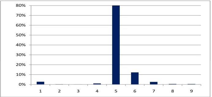
Figure 2: Synthetic example 1: posterior model probabilitiesp(M_k|DI) from 1,000,000

simula-tions.

observe that the RJMCMC algorithm strongly favors model M₄ (with posterior probability

75%) which corresponds to the correct truncation index k = 4. In Figure 3 we provide the

estimates of the development pattern log(γj). We see that the RJMCMC pattern log(E[γj| DI])

3 0 -2.5 -2.0 -1.5

0 1 2 3 4 5 6 7 8 9

-3.5 -3.0 -2.5 -2.0 -1.5

0 1 2 3 4 5 6 7 8 9

gamma_exact gamma_MLE gamma_posterior

Figure 3: Synthetic example 1: true development pattern log(γj), MLE development pattern

log(γ_bM LE

j ) and posterior means log(E[γj| DI]) forj= 0, . . . ,9.

smooths the MLE pattern log(bγ

M LE

j ). It is basically a straight line after the truncation index

k= 4. It has expected posterior slopeE[β| DI] = 0.16 which is slightly less than the true value

of 0.2.

Finally, we calculate the claims reserves and the prediction variance, the results are provided in

claims reserves msep1/2 full modelf(Dc

I|DI) 34,507,772 2,038,016

maximal posterior probability modelf4(D_Ic|DI,M4) 34,515,029 1,991,573 Bayesian ODP model of England et al. [6] 34,887,898 2,083,059

Table 3: Synthetic example 1: resulting claims reserves and prediction variance for the three

models f(Dc

I|DI) (full model), f4(DIc|DI,M4) (model with the highest posterior probability

p(M_k|D_I)) and f9(Dc_I|DI,M9) (model with no smoothing of column parameters γj according

to England et al. [6]).

models: (1) full modelf(Dc

I|DI); (2) modelf4(DcI|DI,M4) with the highest posterior probability

p(M_k|D_I); (3) the individual column parametersγj modelf9(DIc|DI,M9), according to England et al. [6].

Observations.

We observe that the full model and the maximal posterior probability model M₄ give very

similar claims reserves. This is clear because M4 has a posterior probability of 75% and hence

is the dominant sub model in the full model. The Bayesian ODP model clearly deviates from the

other two models, it gives different reserves and has a higher conditional MSEP (which partly

comes from the fluctuation of the posterior development pattern).

If we consider the conditional MSEPs we see that M4 gives a lower value. This low value is

based on the fact thatk= 4 is an optimal truncation level for the parameter reduction. Whereas

the full model also averages over less optimal truncation levels which have a higher conditional

MSEP. Henceforth, we can either go for M₄ or we can go for the full model (and then we also

account for some model uncertainty in the prediction uncertainty analysis).

Finally, we also remark that the RJMCMC algorithm gives the full posterior distribution (4.1).

Therefore we could calculate any other risk measure besides the conditional MSEP.

4.3 Synthetic example 2

For the second synthetic example we basically choose the same set up as in the previous example,

factorsγj we choose an exponential decay

γj = exp{α−jβ}, forj∈ {0, . . . ,3,5, . . . ,9},

with α=−1.5935 and β= 0.2,

andγ4= 12.2%. That is, we choose a straight line for logγj but one column parameter deviates

from this straight line. We then generate data D_I which provides Table 4. For this data we

i/j 0 1 2 3 4 5 6 7 8 9

0 1,794,068 1,428,926 1,278,271 1,285,400 1,509,556 693,145 596,088 420,823 496,766 257,272

1 1,712,508 2,038,374 1,493,193 982,989 1,289,018 722,341 745,301 497,190 539,322

2 2,127,632 1,728,955 1,136,952 1,207,146 1,463,763 761,753 483,590 546,506

3 2,412,364 1,964,107 1,477,259 1,276,313 1,281,865 592,705 722,250

4 2,287,037 1,792,895 1,737,740 1,265,971 1,260,319 876,562

5 2,265,176 2,005,222 1,635,869 1,137,083 1,314,653

6 2,290,865 1,612,424 1,674,967 1,368,915

7 2,268,155 2,527,768 1,605,586

8 2,132,379 1,727,481

9 2,163,595

Table 4: Synthetic example 2: data DI.

can calculate the maximal posterior probability which provides Figure 4. We observe that

30% 40% 50% 60% 70% 80%

0% 10% 20% 30% 40% 50% 60% 70% 80%

1 2 3 4 5 6 7 8 9

Figure 4: Synthetic example 2: posterior model probabilitiesp(M_k|D_I) from 1,000,000 simula-tions.

the RJMCMC algorithm clearly detects that there is something wrong in γ4 and it attaches

with posterior probability of 80% a straight line after that development period, i.e. it strongly

favors model M₅. In Figure 5 we provide the estimates of the development pattern log(γj).

-3.0 -2.5 -2.0 -1.5

0 1 2 3 4 5 6 7 8 9

-4.0 -3.5 -3.0 -2.5 -2.0 -1.5

0 1 2 3 4 5 6 7 8 9

gamma_exact gamma_MLE gamma_posterior

Figure 5: Synthetic example 2: true development pattern log(γj), MLE development pattern

log(γ_bjM LE) and posterior means log(E[γj| DI]) forj= 0, . . . ,9.

logγ4 deviates from the straight line. The MLE has, not surprisingly, more deviations from the

straight line, especially for high development periods where we have only few observations.

4.4 Real data example

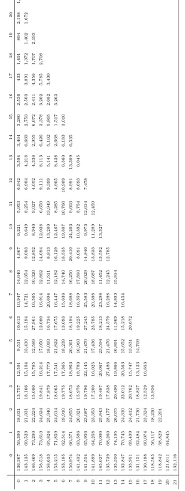
We choose a liability insurance run-off portfolio where we have data for 22 development years j

and accident yearsi. The data is provided in Table 7. Note that we have a very slow run-off of

the liabilities and we would like to fit an exponential decay to late development year parameters

γj for large j.

We choose similar prior distributions ofµiandγj to the previous examples, i.e. as prior mean we

choose the MLEsµ_bM LE_i and _bγ_jM LE with prior uncertaintiess= 100 andv = 1, see (4.4)-(4.5). The distributions of α and β are as in synthetic example 1, i.e. a= −1, σ = 10, b = 0.5 and

τ = 10. The jump rate between the models is driven by v∗ = 100 which provides an average

model jump rate of 14.5% and the proposal parameters in Step (2b) are chosen as

α∗|_α(t) ∼ N(α(t),0.02) and β∗|_β(t) ∼ N(β(t),0.02).

This choice provides an average acceptance rate of 14.6%. Finally, we need to choose the

dispersion parameter ϕ. For this parameter we do an ad-hoc choice using Pearson’s residuals,

see (6.58) in W¨uthrich-Merz [16]. This providesϕ_b= 631.8. Now we have specified all parameters

so that we can apply the RJMCMC Algorithm 3.1 for the Bayesian ODP Model 2.1. We again

20% 30% 40% 50% 60% 70%

0% 10% 20% 30% 40% 50% 60% 70%

1 2 3 4 5 6 7 8 9 10 11 12 13 14 15 16 17 18 19 20 21

Figure 6: Real data example: posterior model probabilities p(M_k|DI) from 1,000,000

simula-tions.

This RJMCMC simulation provides the posterior model probabilities in Figure 6. Figure 6 gives

a rather clear picture that we have an exponential decay in γj after development period k= 7,

i.e. the RJMCMC algorithm favors model M7 with posterior probability of 63%. The reason

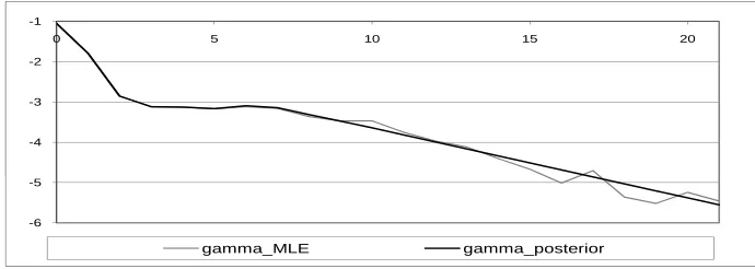
for this strong preference can also be seen in Figure 7 where we plot logγj. In the real data

-4 -3 -2 -1

0 5 10 15 20

-6 -5 -4 -3 -2 -1

0 5 10 15 20

gamma_MLE gamma_posterior

Figure 7: Real data example: MLE development pattern log(γ_bjM LE) and posterior means log(E[γj| DI]) forj= 0, . . . ,21.

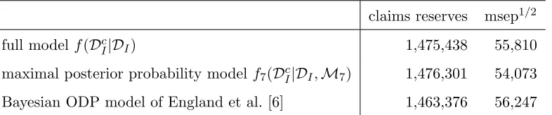
example we then obtain the claims reserves provided in Table 5.

Observations.

approxi-claims reserves msep1/2 full modelf(Dc

I|DI) 1,475,438 55,810

maximal posterior probability model f7(D_Ic|DI,M7) 1,476,301 54,073 Bayesian ODP model of England et al. [6] 1,463,376 56,247

Table 5: Real data example: resulting claims reserves and prediction variance for the three

models f(Dc

I|DI) (full model), f7(DIc|DI,M7) (model with the highest posterior probability

p(M_k|D_I)) and f21(Dc_I|DI,M21) (model with no smoothing of column parametersγj according

to England et al. [6]).

mately the same as the one from the full model. This comes from the fact that in modelM₇ we

obtainE[β|DI,M7] = 0.1746 which is very similar compared to the full modelE[β|DI] = 0.1765.

That is, we obtain about the same decay of the outstanding loss liabilities in model M₇ as in

the full model. Moreover, the maximal posterior probability modelM7 is rather dominant. The

resulting conditional MSEP figures are also very similar between the maximal posterior model

and the full model. The slight difference should not be over-stated.

The Bayesian ODP model of England et al. [6] gives a lower result for the claims reserves which

is mainly caused by the low development parametersγj in periodsj= 16,18,19 (see Figure 7).

Because the full model gives such a clear picture about the truncation index k = 7 we believe

that the Bayesian ODP model under-estimates the outstanding loss liabilities.

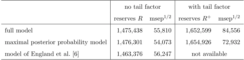
Tail factors.

The data in Table 7 also suggests that there is a claims development beyond development period

j= 21, i.e. we need to estimate a tail factor that accounts for the payments afterj= 21. Using

the exponential decay, we can now easily fit a tail factor to the observed triangle. We denote

the tail factor by

γ+ =

X

j>21

γj =

X

j>21

exp{α−jβ}.

If we assume that, conditionally given all parameters, the payments beyond development year

j= 21 have independent over-dispersed Poisson distributions, i.e.

P

j>21Xi,j

ϕ

ϑ

∼Poi (µi γ+/ϕ),

then we get the predictive distribution including tail factors. The RJMCMC provides then an

empirical approximation to the conditional posterior distribution

In view of (4.2) we obtain the reserves including the tail factor

R+ =

I

X

i=0

∞

X

j=1

E[Xi,j| DI] = I

X

i=0

∞

X

j=1

E[µiγj| DI] = R+ I

X

i=0

E[µiγ+| DI], (4.6)

which is obtained from the RJMCMC sample as in (4.2). In a similar fashion we also obtain the

corresponding conditional MSEP. If we restrict Model Assumptions 2.1 for β to distributions

that are supported on the positive real line, we obtain posterior tail factor

I

X

i=0

E[µiγ+| DI] = I

X

i=0 E



µi

X

j>21

exp{α−jβ}

DI



=

I

X

i=0 E

µi

exp{α−22·β}

1−exp{−β}

DI

,

which is obtained numerically. The results are presented in Table 6.

no tail factor with tail factor

reservesR msep1/2 reservesR+ msep1/2

full model 1,475,438 55,810 1,652,599 84,556

maximal posterior probability model 1,476,301 54,073 1,654,926 72,932

model of England et al. [6] 1,463,376 56,247 not available

Table 6: Real data example: resulting claims reserves and prediction variance for the three

models: full model, model M7) with the maximal posterior probability, and model of England

et al. [6]).

Observations.

We see that the tail factor substantially increases both the claims reserves and the prediction

uncertainty. The claims reserves are increased by R+ −R ≈ 180,000 (or 12% in terms of

R). This gives roughly 8,000 per accident year i∈ {0, . . . ,21}. The increase in the predictive

confidence interval is even 50% or 35%, respectively! We conclude that the tail factor is an

important quantity for this data set, both for the claims reserves but also for the uncertainty in

these claims reserves.

5

Conclusions

This paper has presented an application of RJMCMC methods to an important problem in the

management of general insurance business. The method works very well and allows an automatic

choice to be made, replacing a manual procedure. We believe that this is advantageous and

References

[1] Bj¨orkwall, S., H¨ossjer, O.,Ohlsson, E., Verrall, R.J. (2010). A generalized linear model with

smooth-ing effects for claims reservsmooth-ing. Preprint.

[2] B¨uhlmann, H., De Felice, M., Gisler, A., Moriconi, F., W¨uthrich, M.V. (2009). Recursive credibility

formula for chain ladder factors and the claims development result. Astin Bulletin 39/1, 275-306.

[3] De Jong, P., Zehnwirth, B. (1983). Claims reserving, state-space models and the Kalman filter.

J. Institute Actuaries 110, 157-182.

[4] England, P.D., Verrall, R.J. (2001). A flexible framework for stochastic claims reserving. Proc. CAS

88, 1-38.

[5] England, P.D., Verrall, R.J. (2002). Stochastic claims reserving in general insurance. British

Actu-arial J. 8/3, 443-518.

[6] England, P.D., Verrall, R.J., W¨uthrich, M.V. (2010). Bayesian overdispersed Poisson model and the

Bornhuetter-Ferguson claims reserving method. Preprint.

[7] Gilks, W.R., Richardson, S., Spiegelhalter, D.J. (1996). Markov Chain Monte Carlo in Practice.

Chapman & Hall.

[8] Gisler, A., W¨uthrich, M.V. (2008). Credibility for the chain ladder reserving method. Astin Bulletin

38/2, 565-600.

[9] Green, P.J. (1995). Reversible jump Markov chain Monte Carlo computation and Bayesian model

determination. Biometrika 82/4, 711-732.

[10] Green, P.J. (2003). Trans-dimensional Markov chain Monte Carlo. In: Highly Structured Stochastic

Systems, P.J. Green, N.L. Hjort, S. Richardson (eds.), Oxford Statistical Science Series, 179-206.

Oxford University Press.

[11] Hastings, W.K. (1970). Monte Carlo sampling methods using Markov chains and their applications.

Biometrika 57, 97-109.

[12] Johansen, A.M., Evers, L., Whiteley, N. (2010). Monte Carlo Methods. Lecture notes, Department

of Mathematics, University of Bristol.

[13] Metropolis, N., Rosenbluth, A.W., Rosenbluth, M.N., Teller, A.H., Teller, E. (1953). Equation of

state calculations by fast computing machines. J. Chem. Phys. 21/6, 1087-1092.

[14] Renshaw, A.E., Verrall, R.J. (1998). A stochastic model underlying the chain-ladder technique.

British Actuarial J. 4/4, 903-923.

[15] Verrall, R.J., H¨ossjer, O., Bj¨orkwall, S. (2010). Modelling claims run-off with reversible jump Markov

chain Monte Carlo Methods. Preprint.