Under consideration for publication in J. Fluid Mech. 1
Solving the Boltzmann equation
deterministically by the Fast Spectral
Method: application to gas microflows
Lei Wu
1, Jason M Reese
2, and Yonghao Zhang
1 1James Weir Fluids Laboratory, Department of Mechanical and Aerospace Engineering, University of Strathclyde, Glasgow G1 1XJ, UK
2
School of Engineering, University of Edinburgh, Edinburgh EH9 3JL, UK
(Received ?; revised ?; accepted ?. - To be entered by editorial office)
Based on the fast spectral approximation to the Boltzmann collision operator, we present an accurate and efficient deterministic numerical method for solving the Boltzmann equa-tion. First, the linearised Boltzmann equation is solved for Poiseuille and thermal creep flows, where the influence of different molecular models on the mass and heat flow rates is assessed, and the Onsager-Casimir relation at the microscopic level for large Knudsen numbers is demonstrated. Recent experimental measurements of mass flow rates along a rectangular tube with large aspect ratio are compared with numerical results for the linearised Boltzmann equation. Then, a number of two-dimensional microflows in the transition and free molecular flow regimes are simulated using the nonlinear Boltzmann equation. The influence of the molecular model is discussed, as well as the applicability of the linearised Boltzmann equation. For thermally driven flows in the free molecular regime, it is found that the magnitudes of the flow velocity are inversely proportional to the Knudsen number. The streamline patterns of thermal creep flow inside a closed rectangular channel are analysed in detail: when the Knudsen number is smaller than a critical value, the flow pattern can be predicted based on a linear superposition of the ve-locity profiles of linearised Poiseuille and thermal creep flows between parallel plates. For large Knudsen numbers, the flow pattern can be determined using the linearised Poiseuille and thermal creep velocity profiles at the critical Knudsen number. The critical Knudsen number is found to be related to the aspect ratio of the rectangular channel.
Key words:Authors should not enter keywords on the manuscript
1. Introduction
The Knudsen numberKn, the ratio of the molecular mean free pathλto the charac-teristic flow length`, is an important parameter in rarefied gas dynamics. The Navier-Stokes-Fourier (NSF) equations based on the continuum fluid hypothesis can usually be used up toKn∼0.001†. WhenKnis larger, the continuum hypothesis breaks down and the NSF equations fail to capture the non-conventional behaviour of the rarefied flow. This situation is most frequently encountered in high-altitude aerodynamics and in the vacuum industry (whereλis large), and in micro/nano-electromechanical systems (where
` is small). The Boltzmann equation (BE) is a fundamental model at the microscopic level describing rarefied gas dynamics for the full range of Knudsen number (Cercignani 1990). It uses the velocity distribution function (VDF) defined in a six-dimensional phase space to describe the system state, along with the Boltzmann collision operator (BCO) to model the intermolecular interactions. The BE is complicated, which makes it highly desirable to use macroscopic equations like the NSF model. In the past, Burnett models and Grad moment equations have been derived from the BE. While the Burnett models are intrinsically unstable (Garcia-Colinet al.2008), regularised Grad moment equations have been applied up to the transition flow regime for some specific problems (Gu & Emerson 2009; Ranaet al.2013).
For moderately or highly rarefied gases, it is necessary to solve the BE numerically. The direct simulation Monte Carlo (DSMC) method (Bird 1994) is the prevailing tech-nique. It is efficient for high speed flows, but becomes computationally time-consuming in microflow simulations where the flow velocity is far smaller than the thermal velocity. To tackle this difficulty, information-preservation (Fan & Shen 2001; Masters & Ye 2007) and low-noise (Baker & Hadjiconstantinou 2005; Homolle & Hadjiconstantinou 2007; Radtke et al. 2011) DSMC methods have been proposed. The information-preserving method introduces information quantities (such as the information velocity and information tem-perature) to reduce the statistical noise, which has proven highly effective. However, its convergence to the BE has not been rigorously shown. The low-noise DSMC method significantly improves the computational efficiency of the original DSMC method by sim-ulating only the deviation from the equilibrium state. To our knowledge, for microflow simulations, it is currently the most efficient stochastic method to solve the BE (Radtke et al.2011).
The deterministic numerical solution of the BE is, however, theoretically the best method to resolve small signals, because it is not subject to fluctuations. However, the high computational cost in the approximation of the BCO restricts the number of discrete velocity grids one can use; this does not cause problems when the VDF is smooth, but it does lead to failure at largeKnwhere discontinuities and/or fine structures exist. There-fore, a deterministic numerical method allowing a large number of discrete velocity grids but with reduced computational cost is needed for highly rarefied gas flow simulations.
The Fast Spectral Method (FSM), proposed by Mouhot & Pareschi (2006), and im-proved by Wuet al.(2013), is one such method. The FSM handles the binary molecular collisions in frequency space instead of velocity space, where the Fourier spectrum of the BCO appears as a convolved sum of the weighted spectrum of the VDF. When this sum is carried out directly, the computational cost is O(N6
ξ), where Nξ is the number
of frequency components in one direction. The main idea of the FSM is to separate the frequency components in the weighted function, so that the convolution theorem can be applied, reducing the computational cost toO(M2Nξ3logNξ), where the number of dis-crete anglesM is far less thanNξ. This separation requires special forms of the collision kernel. In our previous paper (Wuet al.2013), these special forms were constructed and validated, making the FSM applicable to all inverse power-law (IPL) potentials (except for the Coulomb potential) and the Lennard-Jones (LJ) potential.
Application of the Fast Spectral Method to gas microflows 3 detail. A new criterion and method is proposed to predict the flow pattern in closed rectangular channels of arbitrary aspect ratio and Knudsen number.
The paper is organized as follows: the BE with special anisotropic collision kernels is introduced in Sec. 2, and the approximation of the (nonlinear and linear) BCOs by the FSM is presented in Sec. 3. In Sec. 4, based on the linearised BE, the numerical accuracy of the FSM is evaluated and its computational efficiency is demonstrated for both Poiseuille and thermal creep flows. The influence of molecular models on the flow rates is discussed and the accuracy of the special collision kernel for the LJ potential is evaluated. In Sec. 5, based on the nonlinear BE, a number of two-dimensional flows are simulated and the influence of the molecular models is compared. A new scaling law for the flow velocity is proposed for thermally driven flows in the free molecular regime. The flow field of the thermal creep flow inside a closed rectangular channel is also investigated. Finally, we conclude this paper in Sec. 6.
2. The Boltzmann equation
2.1. The nonlinear Boltzmann equation
In this paper we consider a monatomic gas. In reality, the intermolecular interaction is best described by the (6-12) LJ potential. For simplicity, however, IPL molecular models have been introduced, and are widely used by researchers. Hence we first consider IPL intermolecular potentials. According to the Chapman-Enskog expansion (Chapman & Cowling 1970), the shear viscosityµis proportional toTω, withT being the temperature and ω the viscosity index. Special collision kernels can be used to recover not only the value of the shear viscosity but also its temperature dependence (Wuet al. 2013). We therefore consider the BE
∂f
∂t +v·
∂f
∂x =Q(f, f∗), (2.1)
where the BCO is given by
Q(f, f∗)≡
Z Z
B(|u|, θ)(f∗0f0−f∗f)dΩdv∗, (2.2)
with the following form of the collision kernel
B(|u|, θ) = |u|
α
K sin
α+γ−1
θ
2
cos−γ θ
2
, (2.3)
whereα= 2(1−ω) andγ is a free parameter.
The BE above is given in dimensionless form: the spatial variable x is normalised by a characteristic flow length `; the molecular velocity v and relative velocity u are normalised by the most probable molecular speedvm=
p
2kBT0/m, withkB the
Boltz-mann constant,T0 the reference temperature, andm the molecular mass. The timet is
normalised by `/vm, while the VDF is normalised byn0/v3m, where n0 is the reference
molecular number density. The subscript∗represents the second molecule in the binary collision, the superscript 0 stands for quantities after the collision, and Ω is the solid angle. Finally, to recover the shear viscosity, we have
K=2
7−ω
5 Γ
α+γ+ 3 2
Γ2−γ 2
Kn, (2.4)
where
Kn= µ(T0)
n0`
r π
2mkBT0
is the unconfined Knudsen number and Γ is the gamma function. Note that the rar-efaction parameterKnis 15π/2(7−2ω)(5−2ω) times larger than the Knudsen number
Knvhs, whereλis defined by equation (4.52) in the book by Bird (1994). Also note that
sometimes the parameterδis used (Sharipov & Seleznev 1994, 1998), which is related to the unconfined Knudsen numberKnby
δ=
√
π
2Kn. (2.6)
For realistic (6-12) LJ potentials, the shear viscosity from the Chapman-Enskog expan-sion is not a power-law function of temperature; only in a small temperature range could the viscosity be described by a single power-law function of temperature. For instance, for helium and argon, in the temperature range 293< T <373, it has been suggested to useω = 0.66 andω = 0.81, respectively (Chapman & Cowling 1970; Bird 1994). For a broader temperature range, the single IPL model may not work well. Note that if we use the realistic collision kernel given by Sharipov & Bertoldo (2009a), the calculation of the weighted function becomes very complicated and, moreover, the efficiency of the FSM is reduced by one order of magnitude. Therefore, we propose using the following collision kernel
B(|u|, θ) =5 P3
j=1bj(kBT0/2)
(αj−1)/2sinαj−1(θ/2)|u|αj/Γ(αj+3
2 )
64√2KnP3
j=1bj(kBT0/)(αj−1)/2
, (2.7)
to approximate that of the realistic (6-12) LJ potential (Wuet al.2013), whereb1= 407.4, b2 =−811.9,b3 = 414.4,α1 = 0.2,α2= 0.1,α3= 0, and is the potential depth. This
expression can recover the shear viscosity for the LJ potential over the temperature range
1< kBT / <25, and produce accurate macroscopic quantities and microscopic VDFs in
normal shock waves when compared to both experimental data and molecular dynamics simulations (Wu et al. 2013). Hereafter, the BE using the approximated collision ker-nel (2.7) will be called the LJ model, and the accuracy of this model in the microflow simulations will be assessed.
2.2. The linearised Boltzmann equation
If the state of the gas is weakly nonequilibrium, the nonlinear BE (2.1) can be linearised. We express the VDF then as
f(t,x,v) =feq+h(t,x,v), (2.8) where
feq(v) = exp(−|v|
2)
π3/2 (2.9)
is the global equilibrium velocity distribution function, andh(t,x,v) represents the de-viation from global equilibrium satisfying|h| 1. The nonlinear BE is then linearised to
∂h
∂t +v·
∂h
∂x =Lg(h)−νeq(v)h, (2.10)
where Lg(h) =
Z Z
B(|u|, θ)[feq(v0)h(v0∗) +feq(v∗0)h(v0)−feq(v)h(v∗)]dΩdv∗, (2.11)
which can be viewed as a linear gain term, and
νeq(v) =
Z Z
Application of the Fast Spectral Method to gas microflows 5 is the equilibrium collision frequency.
3. The Fast Spectral Method
The five-fold integral BCO poses a challenge for the numerical solution of the BE. Un-like the discrete velocity method, which handles the binary collision in velocity space, the FSM works in a corresponding frequency space, where the VDF and BCO are expanded in Fourier series. The discrete velocity grid points can be nonuniform to capture dis-continuities, however, in order to take advantage of fast Fourier transform (FFT)-based convolution, the frequency components should be uniformly distributed, i.e.
f(v) =
N/2−1
X
j=−N/2
ˆ
fjexp(iξj·v),
ˆ
fj= 1
VD
Z
D
f(v) exp(−iξj·v)dv,
(3.1)
wherei is the imaginary unit,N= (N10, N20, N30), the equidistant frequency components areξj=jπ/Lwithj= (j1, j2, j3) andL being the maximum truncated velocity, andD
is the truncated velocity domain withVD its volume. The velocity domain is discretized
byN1×N2×N3 points and the spectrum ˆf of the VDF can be calculated numerically
by the trapezoidal rule. Note that the number of velocity grid points is usually larger than the number of frequency components.
The BCO and its Fourier spectrum ˆQ are also expanded by Fourier series. Thej-th Fourier mode of the BCO is related to the spectrum ˆf as follows (Wuet al. 2013):
ˆ
Q(j) = 1
VD
Z
D
Q(f, f∗) exp(−iξj·v)dv= N/2−1
X
l+m=j l,m=−N/2
ˆ
flfˆm[β(l,m)−β(m,m)], (3.2)
where l = (l1, l2, l3), m = (m1, m2, m3), and β(l,m) is the weighted function. For the
collision kernel (2.3) for IPL potentials, the frequency components ξl and ξm in the weighted function can be separated as
β(l,m)IP L'
4 K M X p,q=1 ψγ nq
|ξm|2−(ξm·eθp,ϕq)
2oω
pωqsinθpφα+γ(ξl·eθp,ϕq), (3.3)
while for the collision kernel (2.7) to approximate the LJ potential, we have
β(l,m)LJ'
5 16√2KnP3
j=1bj(kBT0/)(αj−1)/2 M
X
p,q=1
ψγnq|ξm|2−(ξm·e
θp,ϕq)
2o
×ωpωqsinθp 3
X
j=1
bj(kBT0/2)(αj−1)/2φαj(ξl·eθp,ϕq)/Γ
α
j+ 3
2
,
(3.4) where θp (ϕq) and ωp (ωq) are the p (q)-th point and weight in the Gauss-Legendre quadrature, respectively, with θ, ϕ ∈ [0, π]; eθp,ϕq = (sinθpcosϕq,sinθpsinϕq,cosθp),
φα+γ(s) = 2R R
0 ρ
α+γcos (ρs)dρ, andψγ(s) = 2πRR
0 ρ
1−γJ
0(ρs)dρ. HereR= 2
√
2L/(2 + √
2) is chosen approximately as the average value of its minimum allowed value 2√2L/(3+ √
2) and its maximum allowed value L(see figure 5 in Wuet al. (2013)), andJ0 is the
For conventional spectral methods (Pareschi & Russo 2000; Gamba & Tharkabhushanam 2009), equation (3.2) is calculated by direct sum, with a computational costO(N02
1 N202N302).
However, if the FFT-based convolution is applied, the computational cost is reduced to
O(M2N0
1N20N30log(N10N20N30)). The number of discrete angles M controls the
compu-tational cost and the numerical accuracy. It will be shown below thatM = 6 produces sufficiently accurate results. Hence the FSM is significantly faster than conventional spec-tral methods. Note that the computational cost of the IPL and LJ models are exactly the same.
When the spectrum of the BCO is obtained, we calculate the BCO through the fol-lowing equation:
Q(f, f∗) = N/2−1
X
j=−N/2
ˆ
Q(j) exp(iξj·v). (3.5)
Now we consider the fast spectral approximation of the linearised collision operator. The equilibrium collision frequency can be calculated analytically. For the linearised gain termLg, when the IPL potential is considered, thej-th Fourier mode ofLgis
ˆ Lg(j)≈
4
K M
X
p,q=1
N/2−1
X
l+m=j l,m=−N/2
ωpωq[ ˆfeq(l)φα+γ(ξl, θp, ϕq)]·[ˆhmψγ(ξm, θp, ϕq)]·sinθp
+ 4
K M
X
p,q=1 N/2−1
X
l+m=j l,m=−N/2
ωpωq[ˆhlφα+γ(ξl, θp, ϕq)]·[ ˆfeq(m)ψγ(ξm, θp, ϕq)]·sinθp
− 4
K
N/2−1
X
l+m=j l,m=−N/2
ˆ
feq(l)·[ˆhmφloss],
(3.6) whereφloss=PM
p,q=1ωpωqφα+γ(ξm, θp, ϕq)ψγ(ξm, θp, ϕq) sinθpand ˆhis the spectrum of
the VDF h. For the LJ collision kernel (2.7), the j-th Fourier mode of the linear gain term can be obtained in a similar way.
Note that each term on the right hand side of equation (3.6) is a convolution; like equation (3.2), these can be calculated effectively by a FFT-based convolution. Since the Fourier transform of the terms ˆfeq(l)φα+γ(ξl, θp, ϕq)and ˆfeq(m)ψγ(ξm, θp, ϕq) can
be precomputed and stored, the computational time required for the linearised collision operator is nearly the same as that for the full BCO. However, for IPL potentials, if
γ= (1−α)/2, the linear gain operator is simplified to
Lg(h) =
Z Z
B(|u|, θ)[2feq(v0)h(v0∗)−feq(v)h(v∗)]dΩdv∗, (3.7)
and itsj-th Fourier mode is approximated by
ˆ Lg(j)≈
8
K M
X
p,q=1 N/2−1
X
l+m=j l,m=−N/2
ωpωqfˆeq(l)φα+γ(ξl, θp, ϕq)ˆhmψγ(ξm, θp, ϕq) sinθp
− 4
K
N/2−1
X
l+m=j l,m=−N/2
ˆ
feq(l)·[ˆhmφloss],
(3.8)
Application of the Fast Spectral Method to gas microflows 7 The symmetry in the VDF can also help to reduce computational cost further. For example, ifhis symmetric with respect tov3, i.e.,h(v3) =h(−v3), thenqin equation (3.8)
can only take values of 1,2,· · · , M/2 for even M. We denote the spectrum obtained in this way as ˆLz
g(j) and let Lzg(v) =
P
jLˆ z
g(j) exp(iξj·v). Then the linear gain operator
Lg(v) can be obtained asLzg(v1, v2, v3) +Lzg(v1, v2,−v3). In this way the computational
cost is reduced by half. This technique can also be applied to the nonlinear BCO.
4. Numerical results for Poiseuille and thermal creep flows using the
linearised Boltzmann equation
Poiseuille and thermal creep flows are two classical problems in rarefied gas dynamics. Because of the singular (over-concentration) behaviour in the VDF (Takata & Funagane 2011), the numerical simulation of a highly rarefied gas is a difficult task; for a long time accurate numerical results have been limited toKn620 for the hard sphere gas (Ohwada et al.1989; Doi 2010). Recently, some progress has been achieved both analytically and numerically in obtaining the mass and heat flow rates at large Knudsen numbers (Takata & Funagane 2011; Funagane & Takata 2012; Doi 2012a,b). Here, based on the FSM for the linearised BCO, we solve these two classical flows in parallel plate and rectangular tube configurations up toKn∼106. The accuracy of the FSM for solving the linearised BE is
evaluated by comparing our numerical results for the Poiseuille flow of a hard sphere gas with those obtained by the numerical kernel method (Ohwadaet al.1989). We can then determine the discretization resolutions required in the velocity and frequency spaces, as well as the number of discrete anglesM. The influence of the molecular models on the mass and heat flow rates is discussed below; specifically, we check the model accuracy by comparing flow rates for the IPL and LJ models with those for the realistic LJ potentials presented in Sharipov & Bertoldo (2009b). Finally, the recent experimental data by Ewart et al.(2007) is evaluated.
4.1. Poiseuille flow between parallel plates
Consider a gas between two parallel plates located atx2 =−`/2 and`/2, respectively.
A uniform pressure gradient is imposed on the gas in the x1 direction: the pressure is
given byn0kBT0(1 +βPx1/`) with|βP| 1. The BE is linearised around the equilibrium
state at rest with number densityn0 and temperatureT0, where the VDF is expressed
asf =feq+βP(x1feq+h). The linearised BE in the dimensionless form is then
v2 ∂h
∂x2
=Lg(h)−νeq(v)h−v1feq, (4.1)
and the velocity and heat flux areV1=
R
v1hdvandq1=
R
|v|2−5 2
v1hdv, respectively.
Due to symmetry, only half of the spatial region (−0.5 6x2 60) is simulated, with
a specular-reflection boundary condition at x2 = 0. The diffuse boundary condition is
adopted at the wall, i.e., h(x2 =−0.5, v2 >0) = 0. The spatial domain is divided into Nsnonuniform sections, with most of the discrete points placed near the wall:
x2= (10−15s+ 6s2)s3−0.5, (4.2)
wheres= (0,1,· · ·, Ns)/2Ns. ForNs= 100, the size of the smallest section is 1.24×10⁻⁶, while the largest is 0.0094.
Because of the symmetry and smoothness of the VDF,N1, N3= 12 uniform grids are
Fast spectral method Literature
M = 6 M = 8 M = 12
k −M Q −M Q −M Q −M Q
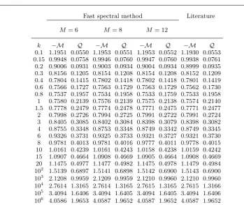
[image:8.595.105.455.122.416.2]0.1 1.1951 0.0550 1.1953 0.0551 1.1953 0.0552 1.1930 0.0553 0.15 0.9948 0.0758 0.9946 0.0760 0.9947 0.0760 0.9938 0.0761 0.2 0.9006 0.0931 0.9003 0.0934 0.9004 0.0934 0.8999 0.0935 0.3 0.8156 0.1205 0.8154 0.1208 0.8154 0.1208 0.8152 0.1209 0.4 0.7804 0.1415 0.7802 0.1418 0.7802 0.1418 0.7801 0.1419 0.6 0.7566 0.1727 0.7563 0.1729 0.7563 0.1729 0.7562 0.1730 0.8 0.7537 0.1957 0.7534 0.1958 0.7533 0.1759 0.7533 0.1958 1 0.7580 0.2139 0.7576 0.2139 0.7575 0.2138 0.7574 0.2140 1.5 0.7778 0.2479 0.7774 0.2478 0.7771 0.2475 0.7771 0.2477 2 0.7998 0.2726 0.7994 0.2725 0.7991 0.2722 0.7991 0.2724 3 0.8405 0.3085 0.8402 0.3084 0.8398 0.3079 0.8398 0.3082 4 0.8755 0.3348 0.8753 0.3348 0.8749 0.3342 0.8749 0.3345 6 0.9326 0.3731 0.9325 0.3733 0.9321 0.3727 0.9321 0.3730 8 0.9781 0.4013 0.9781 0.4016 0.9777 0.4011 0.9778 0.4015 10 1.0161 0.4239 1.0161 0.4243 1.0158 0.4238 1.0159 0.4242 15 1.0907 0.4664 1.0908 0.4669 1.0905 0.4664 1.0908 0.4669 20 1.1475 0.4977 1.1477 0.4982 1.1475 0.4978 1.1479 0.4984 102 1.5139 0.6897 1.5141 0.6898 1.5142 0.6900 1.5143 0.6900 103 2.1208 0.9959 2.1209 0.9959 2.1210 0.9960 2.1210 0.9960 104 2.7614 1.3165 2.7614 1.3165 2.7615 1.3165 2.7615 1.3166 105 3.4094 1.6406 3.4094 1.6405 3.4094 1.6405 3.4094 1.6406 106 4.0586 1.9653 4.0587 1.9652 4.0587 1.9652 4.0587 1.9652
Table 1: Mass and heat flow rates in Poiseuille flow between parallel plates of a hard sphere gas. For k= 8Kn/5√π620 and k>102, the data in the last two columns are collected from Ohwadaet al.(1989) and Takata & Funagane (2011), respectively.
In the discretization ofv2,N2nonuniform grids are used:
v2=
L2
(N2−1)ı
(−N2+ 1,−N2+ 3,· · · , N2−1)ı, (4.3)
whereL2= 4 andıis a positive odd number. Due to the over-concentration in the VDF,
large values ofNsandıshould be chosen when investigating largeKnproblems. The number of frequency components in theξ1andξ3 directions areN10N30 = 24×24,
and there are N20 frequency components in theξ2 direction. The FFT is used in thev1
andv3 directions, while in thev2direction the direct sum is implemented†, resulting in
an overall computational cost of O(N2N20N10N30ln(N10N30)), which is comparable to the
FFT-based convolution sum of equation (3.8).
To obtain the stationary solution, the following implicit iteration scheme is used:
νeq(v)hk+1+v2
∂hk+1
∂x2
=Lg(hk)−v1feq, (4.4)
where∂h/∂x2is approximated by a second-order upwind finite difference. The calculation
of Lg(hk) is as follows: whenhk is known, we obtain ˆLg from equation (3.8). Then we
† For nonuniform velocity grids (4.3), we useP
mg(v2m)wmto approximate
R
g(v2)dv2, where
Application of the Fast Spectral Method to gas microflows 9
10−1 100 101 102 0.7 0.8 0.9 1 1.1 1.2 1.3 1.4 1.5 Kn
0.5 0.6 0.7 0.8 0.9 1 0.75 0.755 0.76 0.765 0.77 0.775 0.78 Hard sphere Argon Maxwell
(a) Mass flow rate−Matαa= 1.0
10−1 100 101 102 0.1 0.2 0.3 0.4 0.5 0.6 0.7 Kn
0.2 0.3 0.4 0.5 0.1
0.12 0.14
(b) Heat flow rateQatαa= 1.0
10−1 100 101 102 0.9 1 1.1 1.2 1.3 1.4 1.5 1.6 1.7 1.8 1.9 2 2.1 K n
(c) Mass flow rate−Matαa= 0.8
10−1 100 101 102 0 0.1 0.2 0.3 0.4 0.5 0.6 0.7 0.8 0.9 K n
[image:9.595.136.453.95.404.2](d) Heat flow rateQatαa= 0.8
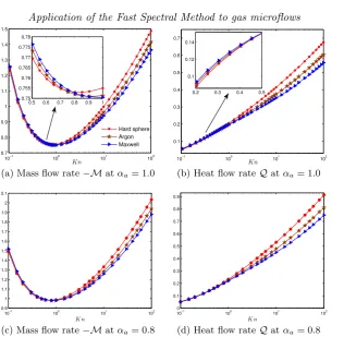
Figure 1: Comparisons of mass and heat flow rates for different IPL molecular models in Poiseuille gas flow between parallel plates. Hereαa represents the wall accommodation
coefficient, where the boundary condition at x2 = −0.5 is h(v1, v2, v3, x2 = −0.5) =
(1−αa)h(v1,−v2, v3, x2=−0.5) forv2>0.
obtainLg(hk) by applying the inverse FFT to ˆLg:Lg(hk) =P N/2−1
j=−N/2Lˆg(j) exp(iξj·v).
The iterations are terminated when changes in the mass flow rate
M= 2 Z 0
−1/2
V1dx2, (4.5)
and heat flow rate
Q= 2 Z 0
−1/2
q1dx2, (4.6)
between two consecutive iteration steps are less than 10−8.
To validate the FSM for the linearised BE, our numerical results are compared to those obtained using the numerical kernel method (Ohwadaet al.1989) for a hard sphere gas (ω= 0.5). Fork= 8Kn/5√π620, the number of equispaced frequency components is
N0
2= 32 and the velocity discretization is given by equation (4.3) withN2= 48 andı= 3.
Fork>100, we chooseN20 = 64,N2= 100, andı= 7. The comparisons are summarised
He Ne Ar Kr Xe
IPL LJ LJ LJ LJ IPL LJ LJ LJ LJ IPL LJ LJ
δ FSM FSM SB FSM SB FSM FSM SB FSM SB FSM FSM SB
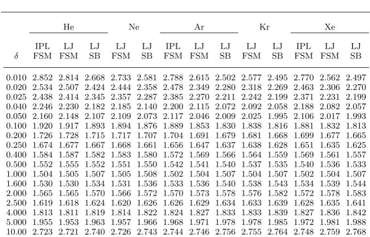
[image:10.595.95.477.117.362.2]0.010 2.852 2.814 2.668 2.733 2.581 2.788 2.615 2.502 2.577 2.495 2.770 2.562 2.497 0.020 2.534 2.507 2.424 2.444 2.358 2.478 2.349 2.280 2.318 2.269 2.463 2.306 2.270 0.025 2.438 2.414 2.345 2.357 2.287 2.385 2.270 2.211 2.242 2.199 2.371 2.231 2.199 0.040 2.246 2.230 2.182 2.185 2.140 2.200 2.115 2.072 2.092 2.058 2.188 2.082 2.057 0.050 2.160 2.148 2.107 2.109 2.073 2.117 2.046 2.009 2.025 1.995 2.106 2.017 1.993 0.100 1.920 1.917 1.893 1.894 1.876 1.889 1.853 1.830 1.838 1.816 1.881 1.832 1.813 0.200 1.726 1.728 1.715 1.717 1.707 1.704 1.691 1.679 1.681 1.668 1.699 1.677 1.665 0.250 1.674 1.677 1.667 1.668 1.661 1.656 1.647 1.637 1.638 1.628 1.651 1.635 1.625 0.400 1.584 1.587 1.582 1.583 1.580 1.572 1.569 1.566 1.564 1.559 1.569 1.561 1.557 0.500 1.552 1.555 1.552 1.551 1.550 1.542 1.541 1.540 1.537 1.535 1.540 1.536 1.533 1.000 1.504 1.505 1.507 1.505 1.508 1.502 1.504 1.507 1.504 1.507 1.502 1.504 1.507 1.600 1.530 1.530 1.534 1.531 1.536 1.533 1.536 1.540 1.538 1.543 1.534 1.539 1.544 2.000 1.565 1.565 1.570 1.566 1.572 1.570 1.573 1.578 1.576 1.582 1.572 1.578 1.583 2.500 1.619 1.618 1.624 1.620 1.626 1.626 1.629 1.634 1.633 1.639 1.628 1.635 1.641 4.000 1.813 1.811 1.819 1.814 1.822 1.824 1.827 1.833 1.833 1.839 1.827 1.836 1.842 5.000 1.955 1.953 1.963 1.957 1.966 1.968 1.971 1.978 1.978 1.985 1.972 1.981 1.988 10.00 2.723 2.721 2.740 2.726 2.743 2.744 2.746 2.756 2.755 2.764 2.748 2.759 2.768
Table 2: Mass flow rate (−2M) in Poiseuille flow of various gases between parallel plates for variousδ, see equation (2.6). The data in columns denoted by SB are those results from Sharipov & Bertoldo (2009b).
& Shen 2001), and found that the information-preserving method works well except at extremely large Knudsen number: the relative error in the mass flow rate between the two methods reaches about 7% atKnvhs= 100.
We now compare the mass and heat flow rates for a hard sphere gas (ω= 0.5), for argon (ω= 0.81), and for a Maxwell gas (ω = 1) using the IPL models. The numerical results are shown in figure 1. We denoteKnc(≈0.9) the Knudsen number at which the Knudsen minimum in the mass flow rate exists. WhenKn > Knc (orKn < Knc), the mass flow rate decreases (or increases) as the viscosity index ω increases, for a fixed value ofKn. For instance, atKn= 10, the mass flow rate of the Maxwell gas is about 94% that of the hard sphere gas when αa = 1. The underlying mechanism for this may be understood in terms of the effective collision frequency: for the same value of shear viscosity, the average collision frequencyRνeq(v)feqdv/R feqdvincreases withω(see figures 12 and 13 in Wuet al. (2013) and the corresponding text therein). Therefore, Maxwell molecules have a greater effective collision frequency (and a smaller effectiveKn) than hard sphere molecules. Since at largeKnthe mass flow rate increases withKn, the Maxwell gas has a lower mass flow rate than the hard sphere gas. Conversely, since at smallKnthe mass flow rate decreases withKn, when Kn < Knc, the Maxwell gas has a higher mass flow
rate than the hard sphere gas, although the difference is very small. The heat flow rate behaves similarly to the mass flow rate; that is, whenKn >0.5 (orKn <0.5), the heat flow rate decreases (or increases) asω increases, for a fixed value ofKn. The difference in flow rates between various gases with the same value of shear viscosity holds when the wall accommodation coefficientαa is not 1, see figure 1(c,d).
Application of the Fast Spectral Method to gas microflows 11
He Ne Ar Kr Xe
IPL LJ LJ LJ LJ IPL LJ LJ LJ LJ IPL LJ LJ
δ FSM FSM SB FSM SB FSM FSM SB FSM SB FSM FSM SB
[image:11.595.96.478.120.364.2]0.010 1.252 1.217 1.142 1.143 1.103 1.185 1.043 1.055 1.013 1.053 1.166 1.001 1.056 0.020 1.092 1.066 1.027 1.006 0.990 1.033 0.924 0.937 0.899 0.933 1.016 0.890 0.935 0.025 1.042 1.020 0.989 0.965 0.954 0.986 0.890 0.900 0.866 0.895 0.970 0.857 0.897 0.040 0.942 0.927 0.909 0.884 0.878 0.893 0.821 0.824 0.801 0.818 0.879 0.793 0.819 0.050 0.897 0.885 0.870 0.847 0.843 0.851 0.790 0.790 0.771 0.782 0.838 0.764 0.783 0.100 0.764 0.761 0.751 0.737 0.734 0.729 0.697 0.689 0.682 0.680 0.719 0.677 0.679 0.200 0.641 0.644 0.637 0.631 0.627 0.617 0.604 0.595 0.593 0.585 0.610 0.589 0.583 0.250 0.604 0.607 0.601 0.597 0.593 0.583 0.574 0.565 0.564 0.556 0.577 0.560 0.554 0.400 0.527 0.531 0.526 0.525 0.521 0.513 0.509 0.503 0.502 0.495 0.509 0.499 0.493 0.500 0.492 0.495 0.491 0.491 0.487 0.480 0.477 0.473 0.473 0.467 0.477 0.470 0.465 1.000 0.386 0.387 0.385 0.386 0.383 0.381 0.381 0.379 0.379 0.377 0.380 0.379 0.376 1.600 0.316 0.316 0.315 0.316 0.314 0.315 0.316 0.315 0.316 0.315 0.315 0.316 0.315 2.000 0.283 0.284 0.282 0.284 0.282 0.284 0.285 0.284 0.286 0.285 0.284 0.286 0.286 2.500 0.252 0.252 0.251 0.252 0.251 0.254 0.255 0.254 0.256 0.256 0.254 0.257 0.256 4.000 0.189 0.189 0.188 0.190 0.189 0.192 0.193 0.193 0.195 0.196 0.193 0.196 0.197 5.000 0.162 0.162 0.161 0.163 0.162 0.166 0.166 0.166 0.168 0.169 0.167 0.169 0.170 10.00 0.094 0.093 0.093 0.094 0.093 0.097 0.097 0.097 0.099 0.099 0.098 0.100 0.100
Table 3: Heat flow rate (2Q) in Poiseuille flow of various gases between parallel plates for various δ. The data in columns denoted by SB are those results from Sharipov & Bertoldo (2009b).
10−2 10−1 100 101 0
2 4 6 8 10 12
δ
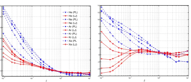
He (PL) He (LJ) Ne (PL) Ne (LJ) Ar (PL) Ar (LJ) Kr (PL) Kr (LJ) Xe (PL Xe (LJ)
10−2
10−1
100
101 −6
−4 −2 0 2 4 6 8 10 12 14
δ
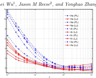
Figure 2: Relative differences in the mass (left) and heat (right) flow rates between the molecular models and LJ potentials in Poiseuille gas flow between parallel plates for variousδ.
[image:11.595.97.483.417.583.2](a) Atx2=−0.5 (b) Atx2=−0.25 (c) Atx2= 0
Figure 3: Demonstration of the Onsager-Casimir relation at the microscopic level. Lines (or dots): velocity distribution functions (|v|2−5
2)hP in Poiseuille flow (orhT in thermal
creep flow) atv1, v3= 6/31 andKn= 104. From top to bottom, the curves correspond
to the hard sphere, helium (IPL), argon (IPL), and Maxwell gases, respectively.
heat flow rates produced by the FSM and those in Sharipov & Bertoldo (2009b) are visualized in figure 2. Forδ >0.2, the relative difference|MIP L− MSB|/|MSB|between
the IPL models and LJ potentials is less than 1%. For δ < 0.2, the relative difference increases asδdecreases. Specifically, atδ= 0.01, the IPL model overestimates the mass flow rate by around 6.9%, 10.5%, 11.4%, 11.7%, and 11.0% for He, Ne, Ar, Kr, and Xe, respectively. When the collision kernel (2.7) is used for the LJ potential, at δ = 0.01, the LJ model overestimates the mass flow rate by around 5.5%, 6.0%, 4.5%, 3.3%, and 2.6% for He, Ne, Ar, Kr, and Xe, respectively. As δ increases, the relative difference quickly decreases. Similar behaviour can be observed for the heat flow rate, except that the LJ models for Ar, Kr, and Xe underestimate the heat flow rate at small values ofδ. Generally speaking, when compared to the solution for the realistic LJ potential, the LJ model yields closer results than the IPL model.
4.2. Thermal creep flow between parallel plates
In thermal creep flow, the wall temperature varies asT =T0(1+βTx1/`), where|βT| 1.
The VDF is expressed asf =feq+βT[x1feq(|v|2−52) +h] and the linearised BE is given
by equation (4.1) with the last term replaced byv1(|v|2−52)feq.
The Onsager-Casimir relation (Loyalka 1971; Sharipov 1994a,b; Takata 2009a,b) states that the mass flow rate in thermal creep flow is equal to the heat flow rate in Poiseuille flow:R
V1[hT]dx2=
R
q1[hP]dx2. Recently, Takata & Funagane (2011) observed a strong
relation, that is, at large Kn, V1[hT] and q1[hP] have identical spatial profiles, i.e., V1[hT] =q1[hP] +O[Kn−1(lnKn)2]. The VDFs obtained by our FSM in figure 3 show
that a stronger Onsager-Casimir relation exists at the microscopic level, that is,hT ≈
(|v|2−5
2)hP, at largeKn, for various IPL models.
Because of the Onsager-Casimir relation, we compare only the heat flow rates in ther-mal creep flow for different potential models. The results are in Table 4. For a particular molecular model, the heat flow rate increase monotonically as δ decreases. As in the Poiseuille flow case, different molecular models have different flow rates at the same value of shear viscosity; for IPL models, the heat flow rate always decreases asω increases.
The relative difference in heat flow rates is visualized in figure 4. Atδ= 0.01, for He, Ne, Ar, Kr, and Xe, the IPL models overestimate the heat flow rate relative to Sharipov & Bertoldo (2009b) by 6.6%, 10.3%, 11.4%, 11.7%, and 11%, while the LJ model over-estimate the heat flow rate by 5.1%, 5.7%, 4.6%, 3.5%, and and 2.9%, respectively. Asδ
Application of the Fast Spectral Method to gas microflows 13
He Ne Ar Kr Xe
IPL LJ LJ LJ LJ IPL LJ LJ LJ LJ IPL LJ LJ
δ FSM FSM SB FSM SB FSM FSM SB FSM SB FSM FSM SB
[image:13.595.100.476.128.363.2]0.010 6.269 6.182 5.879 6.010 5.684 6.140 5.768 5.512 5.691 5.496 6.104 5.662 5.500 0.020 5.496 5.435 5.263 5.301 5.121 5.385 5.109 4.958 5.048 4.934 5.354 5.024 4.935 0.025 5.255 5.202 5.059 5.082 4.936 5.151 4.906 4.779 4.850 4.754 5.121 4.828 4.754 0.040 4.761 4.725 4.626 4.632 4.542 4.670 4.491 4.404 4.445 4.376 4.644 4.427 4.373 0.050 4.532 4.505 4.421 4.424 4.353 4.448 4.298 4.225 4.257 4.197 4.424 4.240 4.193 0.100 3.848 3.840 3.792 3.793 3.761 3.784 3.709 3.669 3.679 3.641 3.766 3.666 3.635 0.200 3.196 3.200 3.174 3.175 3.162 3.151 3.120 3.103 3.098 3.080 3.138 3.089 3.074 0.250 2.992 2.997 2.977 2.977 2.968 2.951 2.929 2.918 2.909 2.897 2.940 2.901 2.891 0.400 2.569 2.575 2.562 2.562 2.560 2.538 2.526 2.525 2.511 2.508 2.529 2.504 2.502 0.500 2.371 2.377 2.367 2.367 2.366 2.343 2.335 2.337 2.321 2.322 2.336 2.316 2.317 1.000 1.772 1.776 1.770 1.770 1.771 1.752 1.750 1.756 1.741 1.745 1.748 1.737 1.741 1.600 1.387 1.391 1.385 1.387 1.387 1.373 1.371 1.377 1.365 1.369 1.369 1.362 1.366 2.000 1.216 1.219 1.213 1.215 1.216 1.203 1.202 1.207 1.197 1.201 1.200 1.194 1.198 2.500 1.054 1.057 1.051 1.054 1.053 1.043 1.042 1.046 1.038 1.041 1.040 1.036 1.039 4.000 0.752 0.754 0.750 0.752 0.752 0.745 0.745 0.747 0.742 0.744 0.743 0.740 0.743 5.000 0.631 0.633 0.629 0.631 0.630 0.625 0.625 0.627 0.622 0.625 0.623 0.621 0.624 10.00 0.347 0.348 0.345 0.347 0.346 0.344 0.344 0.345 0.343 0.344 0.343 0.342 0.344
Table 4: Heat flow rate (2Q) in thermal creep flow of various gases between parallel plates for variousδ. The data in columns denoted by SB are those results from Sharipov & Bertoldo (2009b).
for Poiseuille flows, indicate that, in the free-molecular regime, it is necessary to consider the LJ potential to get highly reliable results (Sharipov & Strapasson 2012; Venkattra-man & Alexeenko 2012; Sharipov & Strapasson 2013). However, the LJ model with the collision kernel (2.7) can produce mass and heat flow rates with a relative error less than 2% whenδ >0.04 or, equivalently,Kn <22.
In the free molecular limit, it has previously been found that the mass flow rates in Poiseuille and thermal creep flows increase logarithmically with the Knudsen num-ber (Cercignani & Daneri 1963; Takata & Funagane 2011). Our numerical results show that the heat flow rate in thermal creep flow can also be fitted to a logarithmic function ofKn, viz,Q[hT] =−0.6345 ln(Kn)− Q0 in the region 105< Kn <2×10⁶, where the
constantQ0is 0.2679, 0.1762, 0.07371, and -0.09903 for hard sphere, helium, argon, and
the Maxwell gases when the IPL model is used, respectively.
4.3. Poiseuille and thermal creep flow along a rectangular tube
We now consider rarefied gases in a long straight tube that lies along thex3axis. The cross
section is uniform and rectangular, so that−A`/2< x1 < A`/2 and−`/2 < x2 < `/2,
whereA is the aspect ratio. The linearised BE in dimensionless form for Poiseuille flow along this rectangular tube is:
v1 ∂h
∂x1
+v2 ∂h
∂x2
=Lg(h)−νeq(v)h−v3feq, (4.7)
whilev3should be replaced byv3 |v|2−52for the thermal creep flow. Due to symmetry,
10−2
10−1
100
101 0
2 4 6 8 10
δ
[image:14.595.187.386.102.263.2]He (PL) He (LJ) Ne (PL) Ne (LJ) Ar (PL) Ar (LJ) Kr (PL) Kr (LJ) Xe (PL) Xe (LJ)
Figure 4: Relative difference in the heat flow rate between the molecular models and LJ potentials in thermal creep flow between parallel plates as a function ofδ.
(4/A)R0
−1/2
R0
−A/2V3dx1dx2 and the heat flow rate is Q = (4/A)
R0
−1/2
R0
−A/2q3dx1dx2,
whereV3=
R
v3hdvandq3=
R
|v|2−5 2
v3hdv.
This problem was first solved for a hard sphere gas by the numerical kernel method (Doi 2010) and then by the low-noise DSMC method (Radtke et al. 2011). To compare the numerical accuracy and efficiency of our new FSM, we first consider the thermal creep flow
atKnvhs= 0.1 andA= 2. We use a 50×50 nonuniform spatial grid (see equation (4.2)),
32×32 nonuniform velocity grids (equation (4.3) withı= 3) in thev1andv2directions,
and 12 uniform mesh points in thev3direction. The FSM withM = 6 yieldsM= 0.0478,
compared to 0.048 by Doi (2010) and 0.0473 by Radtkeet al.(2011). We then consider Poiseuille flow in the square tube; with a 25×25 spatial cell mesh, 32×32×24 frequency components, andM = 6, we obtainM= 0.3808 and 0.3966,Q= 0.1365 and 0.1874 for
Knvhs = 1 and 10, respectively, compared to Doi’s 0.381 and 0.396 for M, and 0.136
and 0.187 forQ. The computational time is 100 and 40seconds†, respectively, compared to the low-noise DSMC that takes 66 and 12minutes‡, respectively. These comparisons indicate that the FSM is an accurate and efficient new numerical method.
We observe that the difference in mass and heat flow rates between different molecular models is very small whenA= 1. Although the difference increases withA, atA= 10, |(MAr− MHe)/MAr|is only 1.6% atδ= 0.01, while that atA=∞is 7.6%, when the
LJ model is used. So, in the following numerical simulation we only use the IPL model. We now compare our numerical results with recent experiments on the reduced mass flow rate in Poiseuille flow (Ewart et al. 2007). The tube cross section is rectangular, with an aspect ratio ofA= 52.45. The working gas is helium and we take the IPL model withω= 0.66. In the spatial discretization, 100 and 50 nonuniform grid points are used in thex1 and x2 directions, respectively. The number of velocity grids is 32×32×12,
the frequency components are 32×32×24, and the number of discrete angles isM = 6. Different wall accommodation coefficients αa are used: the wall boundary condition is given by h(v1, v2, v3, x1, x2 =−1/2) = (1−αa)h(−v1, v2, v3, x1, x2 =−1/2) forv1 >0
and h(v1, v2, v3, x1 = −A/2, x2) = (1−αa)h(v1,−v2, v3, x1 = −A/2, x2) for v2 > 0.
† Our Fortran program runs on a computer with an Intel Xeon 3.3 GHz CPU, and only one core is used.
Application of the Fast Spectral Method to gas microflows 15
10−2 10−1 100 101
1.4 1.5 1.6 1.7 1.8 1.9 2 2.1 2.2 2.3 2.4 2.5 2.6 2.7 2.8 2.9 3
δm= √π 2K n
G
Experiment αa= 1.00
αa= 0.95
[image:15.595.154.416.133.335.2]αa= 0.92
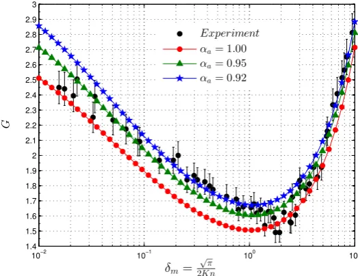
Figure 5: Comparison of the FSM-calculated reduced mass flow rateGin Poiseuille flow along a rectangular tube (aspect ratio 52.45) with the experimental data of Ewartet al. (2007), for various values of the wall accommodation coefficientαa.
The obtained mass flow rateMis transformed to the reduced mass flow rate Gvia the following equation (Sharipov & Seleznev 1994):
G(δin, δout) = 2
δout−δin
Z δout
δin
M(δ)dδ, (4.8)
where the subscripts ‘in’ and ‘out’ stand for the inlet and outlet, respectively. The re-duced mass flow rate G no longer depends on the local pressure gradient, but only on the mean value of pressure; so the parameter δm at the mean pressure of the tube is also introduced. We consider the published experimental data where the inlet to outlet pressure ratio is five, so that δin = 5δm/3 and δout = δm/3. The mass flow rate M is obtained at discrete values of the rarefaction parameter. The reduced mass flow rate is calculated by equation (4.8), where M at an unknownδ is obtained by cubic inter-polation. Comparisons between the numerical and experimental data are visualized in figure 5. Whenδ>6, the experimental data agrees well with the numerical results from the BE if αa = 0.92. In the region 16 δ < 6, the experimental data agrees with the
numerical results ifαa = 0.92∼1. For 0.2 6 δ 61, the mass flow rates from the BE
withαa= 0.92 agree with the experimental measurements. Whenδ60.1, the BE with
αa = 0.95∼1 agrees well with the experimental results.
Note that the advantage of the FSM over the DSMC method becomes more profound for a series of simulations with the same spatial geometry but different values of Kn. SortingKnin descending order, the converged VDF at the previousKncan be used as the initial condition for the FSM for those subsequentKn. In this way, the computational efficiency can be improved further. For example, for this Poiseuille flow problem, it takes 4.4 hours to compute the solution for Kn = 0.1 when the initial VDF is the global equilibrium one, but only 2 hours when the initial VDF is taken as the solution at
Figure 6: Temperature contours and streamlines (velocity: first column; heat flux: second column) in the lid-driven cavity flow of argon gas. From top to bottom, the Knudsen numberKnvhsin each column is 0.1, 1, and 10, respectively. Here and after, the abscissa represents thex1-axis, while the ordinate represents the x2-axis.
5. Numerical results for the nonlinear Boltzmann equation
veloc-Application of the Fast Spectral Method to gas microflows 17
0 0.1 0.2 0.3 0.4 0.5 0.6 0.7 0.8 0.9 1 −0.2 −0.15 −0.1 −0.05 0 0.05 0.1 0.15 0.2 V2 / Vw a ll x1
0 0.1 0.2 0.3 0.4 0.5 0.6 0.7 0.8 0.9 1
−3 −2.5 −2 −1.5 −1 −0.5 0 0.5 1 1.5 2 q2 × 1 0 3 x1
(a) Atx2= 0.5
−0.20 −0.1 0 0.1 0.2 0.3 0.4 0.5 0.6 0.7 0.1 0.2 0.3 0.4 0.5 0.6 0.7 0.8 0.9 1 x2
V1/Vwall
−6 −4 −2 0 2 4 6 8 10 12 14
0 0.1 0.2 0.3 0.4 0.5 0.6 0.7 0.8 0.9 1 x2 q1×103
(b) Atx1 = 0.5
0 0.1 0.2 0.3 0.4 0.5 0.6 0.7 0.8 0.9 1
271 271.5 272 272.5 273 273.5 274 274.5 275 275.5
x1, x2
Temperature
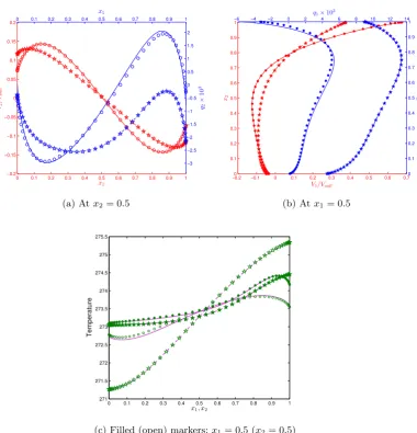
[image:17.595.109.490.122.518.2](c) Filled (open) markers:x1= 0.5 (x2= 0.5)
Figure 7: Comparisons of the velocity, heat flux, and temperature profiles between argon and hard sphere gases in lid-driven cavity flow. The solid (or dashed) lines are the results for argon with Knvhs = 0.1 (or 10). The circles (or stars) are the results for the hard sphere gas withKnvhs= 0.132 (or 13.2).
ities in thermally driven flows in the free molecular regime. Specifically, thermal creep flow inside a closed channel is analysed, where the flow pattern can be well explained by the superposition of both the velocity profiles of linearised Poiseuille and thermal creep flow between parallel plates.
5.1. Lid-driven cavity flow
lid is so small that the linearised BE can be applied, the low-noise DSMC method (Radtke et al.2011) takes more than 1 day to achieve reasonably resolved results atKnvhs= 0.1.
We solve this problem (for argon gas, the upper lid velocity of 50m/s, and a wall temperature of 273K) in a 51×51 nonuniform spatial grid, see equation (4.2). The minimum length of the spatial cell is 7.8×10⁻⁵, while the maximum is 0.0375, with most
of the grid points located near the walls. ForKnvhs= 0.1 and 1, 32×32×12 grid points in velocity space are used, while forKnvhs= 10, there are 64×64×12 velocity grid points, with most of the grid points located in v1, v2 ∼0 to capture the discontinuities in the
VDF. The number of frequency components is 32×32×24. The BCO is approximated by the FSM with M = 6, and the spatial derivatives are approximated by second-order upwind finite differences. We solve the discretized BE by the implicit scheme in an iterative manner. At the (k+ 1)-th iteration step, the VDF at the wall (entering the cavity) is determined according to the diffuse boundary condition, using the VDF at the same position (but leaving the cavity) at the previous iteration step. This numerical scheme is much faster than an explicit time-dependent technique because no Courant-Friedrichs-Lewy condition is imposed (Frangiet al.2007). However, the disadvantage to the explicit time-marching technique is that, when the mass flux entering the cavity at the (k+ 1)-th step (which is equal to that leaving the cavity at the k-th step) is not equal to that leaving the cavity at the (k+ 1)-th step, the total mass inside the cavity is not conserved. To overcome this, at the end of each iteration step, a simple correction of the VDF by a factor equal to the initial total mass divided by the current total mass is introduced. This is sufficient to recover the correct steady state conditions, and was introduced by Mieussens & Struchtrup (2004).
The convergence rate of our iterative scheme is proportional to the Knudsen number.
ForKnvhs = 0.1 and 1, starting from the global equilibrium state, the FSM takes 110
and 14 minutes, respectively, to produce a converged solution, which is when the error between two consecutive iteration steps,
||||2=max
s
R
|V1k+1−Vk
1|2dx1dx2
R |Vk
1|2dx1dx2 ,
s R
|V2k+1−Vk
2|2dx1dx2
R |Vk
2|2dx1dx2
, (5.1)
is less than 10−5.
Figure 6 shows the calculated temperature contours and streamlines in the lid-driven cavity flow of argon gas with diffuse boundary conditions. Compared to DSMC, these solutions are free of noise. We have also simulated the flow of a hard sphere gas, with the same values of the normalized wall velocity (i.e. 0.148) and shear viscosity (the Knudsen numberKnare the same, butKnvhsare different). Comparisons of the velocity, temperature, and heat flux profiles between the two IPL molecular models are shown in figure 7, and demonstrate that the molecular model has little influence on the flow pattern. This may explain why, for the same problem, the Bhatnagar-Gross-Krook and Shakhov kinetic models can both produce excellent results that are in agreement with DSMC data (Huanget al.2012).
5.2. Thermally driven flows 5.2.1. Thermal creep flow inside a closed channel
Application of the Fast Spectral Method to gas microflows 19
(a)Kn= 0.08
(b)Kn= 0.2
(c)Kn= 0.25
(d)Kn= 0.6
(e)Kn= 2
[image:19.595.130.447.106.680.2](f)Kn= 10
50 60 80 100 150 200 300 400 500 600 800 1,000 10−5
10−4
K n R¯V
1
(
x
2
=
0
.
5
)
d
x
1
hard sphere
argon
Maxwell
(a)
−12 −10 −8 −6 −4 −2 0 2 4 6
x 10−3
0 0.05 0.1 0.15 0.2 0.25 0.3 0.35 0.4 0.45
V1×K n x2
hard sphere Kn=1000 hard sphere Kn=100 argon Kn=1000 argon Kn=100 Maxwell Kn=1000 Maxwell Kn=100
(b)
Figure 9: (a) The average horizontal velocity varying withKnin thermal creep flow inside the closed rectangular channel, in the free molecular regime. In this double logarithmic diagram, the three lines have a slope of 1, demonstrating that the velocity magnitude is proportional to 1/Kn. (b) Examples of the linear scalability of the horizontal velocity at
x1= 1.4825.
presents the resulting streamlines and the temperature distributions inside the channel for the flow of argon gas. Due to symmetry, only half of the spatial domain is shown. Unlike thermal creep in an open channel, where the flow straightforwardly moves towards the hot region, the thermal creep flow in a closed channel exhibits richer phenomena. At
Kn= 0.08, the gas flows from the cold region to the hot region along the bottom wall, and returns in the central region. AtKn= 0.2, the flow still moves from hot to cold in the central region, however, near the lower wall the flow moves towards the hot region when x1 < 2 and towards the cold region for at x1 > 2, i.e., a circulation emerges
near the lower corner of the domain. AtKn= 0.25, the circulation near the lower wall grows, which divides the flow in the central region into two circulation zones. The lower circulation zone keeps expanding, and pushes the other two circulations in the central region towards the left and right boundaries, as Kn increases. At Kn = 0.6, the flow direction is reversed (as compared to that whenKn= 0.08) and only one circulation zone remains near the left wall. The reversal of the flow direction persists but the circulations near the left wall gradually disappear as the Knudsen number increases further, for instance, toKn= 2. ByKn= 10, the gas near the bottom wall moves from hot to cold, and two clockwise circulations emerge near the left and right sides. Finally, when the flow enters the free molecular regime, the streamline pattern does not change, but the velocity magnitudes are proportional to 1/Kn, see figure 9. The magnitudes of density, pressure, and temperature, however, remain unchanged irrespective of the Knudsen number.
Comparison of the velocity profiles for different molecular models at the start and the end of the transition flow regime are shown in figure 10; it can be seen that the molecular model affects the velocity magnitudes significantly.
[image:20.595.99.463.103.266.2]Application of the Fast Spectral Method to gas microflows 21
0 0.5 1 1.5 2 2.5 3 3.5 4 4.5 5
−18 −16 −14 −12 −10 −8 −6 −4 −2 0 2 V1 × 1 0 4 x1
0 0.5 1 1.5 2 2.5 3 3.5 4 4.5 5
−0.5 0 0.5 1 1.5 2 2.5 3 3.5 4 V1 × 1 0 4 x1 hard sphere argon Maxwell
(a) Velocity along the central horizontal line
−200 −15 −10 −5 0 5 10 15 20
0.05 0.1 0.15 0.2 0.25 0.3 0.35 0.4 0.45 0.5 x2
V1×104
−12 −10 −8 −6 −4 −2 0 2 4
0 0.05 0.1 0.15 0.2 0.25 0.3 0.35 0.4 0.45 0.5 x2 V1×104
[image:21.595.106.474.102.266.2](b) Velocity along the central vertical line
Figure 10: Velocity profiles for thermal creep flow within a closed rectangular channel;
Kn= 0.08 and 10 are represented by the red and blue lines, respectively.
−0.020 −0.015 −0.01 −0.005 0 0.005 0.01
0.05 0.1 0.15 0.2 0.25 0.3 0.35 0.4 0.45 0.5
V1[hT]−V1hP]M[hT]/M[hP]
x
2
K n= 20√π
10√π
2√π √π √π /2 √π /4 √π /5 √π /8 √π /10 √π /20 √π /40 √π /80
Figure 11: Net velocity profiles obtained by linear superposition of the velocity profiles of Poiseuille and thermal creep flows between parallel plates, which result in zero mass flow rate. The walls are at x2 = 0 andx2 = 1 and the working gas is argon, where the
IPL model withω= 0.81 is used.
is zero. The horizontal velocity profile can be analysed by assuming the wall temperature gradient to be small (i.e. the channel is long enough) so that the BE can be linearised. In this case, we can directly use the velocity profiles obtained in Sec. 4. Figure 11 plots the net velocity profiles in the linear superposition of Poiseuille and thermal creep flows between parallel plates where the net mass flow rate is zero. The flow velocities are normalised; in real problems, the horizontal velocity is given by (see the first paragraph in Sec. 4.2):
V1=βT
V1[hT]−
M[hT]
M[hP]V1[hP]
, (5.2)
whereβT is the temperature gradient; in this case, it is about 1/5.
[image:21.595.176.402.311.493.2]0 0.1 0.2 0.3 0.4 0.5 0.1
0.2 0.3 0.4 0.5
0 0.2 0.4 0.6 0.8 1
0.1 0.2 0.3 0.4 0.5
0 0.125 0.25
0.1 0.2 0.3 0.4 0.5
(d)
0 0.2 0.4 0.6 0.8 1 1.2 1.4 1.6 1.8 2
[image:22.595.139.430.102.299.2]0.1 0.2 0.3 0.4 0.5
Figure 12: Thermal creep flow patterns of the argon gas (IPL model withω = 0.81) in the free molecular regime at different values of length-to-height ratio A. (a) A = 0.25, (b)A= 0.5, (c)A= 1, and (d)A= 2.
positive whenx2<0.25 and negative otherwise, which agrees well with the flow pattern
in figure 8(a). Also, from figure 10(a) we find that, atKn= 0.08,V1(x2= 0.5)' −0.0018
near the left side of the channel, which is well predicted by equation (5.2) when we choose
Kn=√π/20 andx2= 0.5:V1(x2= 0.5)'(−0.009)/5 =−0.0018. Furthermore, as Kn
increases, the magnitude of the horizontal velocity at x2 = 0.5 decreases (figure 11).
This is in accordance with the horizontal velocity profiles shown in figure 10(a), where the velocity magnitude decreases asx1increases from 1 to 4, because the local Knudsen
number increases along the channel as a result of increasing temperature and decreasing particle number density. When Kn = √π/10 (and √π/8), the net horizontal velocity in figure 11 is positive when 0.26 > x2 >0.009 (and 0.28 > x2 >0.023) and negative
otherwise. This explains the flow patterns at the right side of the channel, as shown in figure 8(b). As Knincreases, the extent of the region near the bottom wall where the velocity is negative increases (figure 11), so that the circulation near the bottom wall in figure 8(c) is larger than that in figure 8(b). WhenKnincreases above a critical value of around√π/5, the horizontal velocity in figure 11 is negative whenx2 is smaller than
some fixed valuex2c and positive otherwise. In this case, the flow direction is completely
reversed in comparison with that at small Knudsen numbers. When Kn > √π/2, the fixed value isx2c = 0.2. In figure 8(d-f), we see that the gas moves from left to right if x2<0.2, and moves right to left ifx2>0.2.
Application of the Fast Spectral Method to gas microflows 23 with the length-to-height ratioAof the channel:
Knc'0.35A. (5.3)
For instance, whenA= 0.25, the end effect becomes dominant whenKnc >0.09, and the flow pattern at KnKnc is similar to the flow pattern at Knc. Figure 11 shows that atKn= 0.09 the molecules move from left to right near the bottom wall, and return to the left at x2 = 0.5, which is exactly the case shown in figure 12(a). For A = 0.5, Knc= 0.18'√π/10, and from figure 11 we see the horizontal flow velocity turns from negative to positive and then back to negative as we move from the bottom wall to the central region, which is the same as in figure 12(b). The aspect ratio A = 1 is a critical case, since nearKnc= 0.35'√π/5, the horizontal velocity atx2= 0.5 could be
negative or positive, depending on whether the local Knudsen number is smaller or larger than√π/5. That is why the flow pattern shown in figure 12(c) is more complicated. For
A= 2, whereKnc= 0.7, the flow pattern is simpler, and the molecules move from the
hot to the cold region near the bottom and return from the cold to the hot region near
x2= 0.5, see figure 12(d). ForKn < Knc, the horizontal velocity profiles can be analysed
using the data in figure 11.
5.2.2. Flow induced by a spatially-periodic wall temperature
Consider the gas flow between two parallel plates that have spatially-periodic tem-perature: the upper (x2 = `) and lower plates (x2 = 0) have the temperature T0(1−
0.5 cos 2πx1). Due to symmetry, the spatial domain is chosen as 06x1, x2 61/2. The
specular reflection boundary condition is chosen for the left, upper, and right boundaries, while the diffuse boundary condition is employed at the lower wall. Using the mean den-sity, mean temperatureT0, and the wall distance`, the unconfined Knudsen numberKn
is chosen to be 0.1, 1, and 10. In the spatial discretization, 51 equispaced points are used in thex1 direction and 51 non-uniform points (see equation (4.2)) are placed in thex2
direction, with most of the points close to the lower wall. In the discretization of the velocity space, 64×64×16 (maximum velocity L= 7.5,L2= 5 in equation (4.3) with ı= 3) grid points are used when Kn= 0.1 and 1, while 128×128×16 grid points are used whenKn= 10. The number of frequency components is 32×32×32. Even with such a large number of velocity grid points, the FSM withM = 6 takes only about 150 minutes to converge to||||2 less than 10−5at Kn= 0.1.
The temperature contours and velocity streamlines are shown in figure 13. The gas moves from the cold to the hot region near the lower wall, while it returns from hot to cold around the central horizontal region. The circulation centre approaches the lower wall asKnincreases. The marginal VDFs, which become more complicated asKnincreases, are shown in figure 14, and large discontinuities at the lower wall and fine structures are clearly seen. This demonstrates the necessity of using a large number of velocity grid points in the v1 and v2 directions at large Kn, in order to get a high resolution. The
flow velocities for different molecular models are compared in figure 15: the maximum velocity increases with the viscosity index. We have also investigated the flow in the free molecular regime and find that the velocity magnitudes are inversely proportional to the Knudsen number, as in the case of thermal creep flow inside closed channels.
(a)Kn= 0.1 (b)Kn= 1
[image:24.595.93.471.103.445.2](c)Kn= 10
Figure 13: Contour plots of the temperature, and the velocity streamlines in argon gas subjected to a spatially-periodic wall temperature.
(a)Kn= 1 (b)Kn= 10
Figure 14: Contour plots of the marginal VDF,R f dv3, for Kn= 1 and Kn= 10. In
[image:24.595.103.476.485.670.2]Application of the Fast Spectral Method to gas microflows 25
0 0.1 0.2 0.3 0.4 0.5
0 0.5 1 1.5 2 2.5 3 3.5 4 4.5x 10
−3
x1
V1
Hard sphere: nonlinear Hard sphere: linear Argon: nonlinear Argon: linear Maxwell: nonlinear Maxwell: linear
(a) Atx2= 0
0 0.2 0.4 0.6 0.8 1 1.2 1.4 1.6 x 10⁻³ 0
0.05 0.1 0.15 0.2 0.25 0.3 0.35 0.4 0.45 0.5
V2
x2
[image:25.595.111.476.100.284.2](b) Atx1= 0.5
Figure 15: Comparisons of the velocity profiles predicted by the full nonlinear and the linearised BEs, and for different molecular models. The unconfined Knudsen number is
Kn= 1 and the temperature of the top and bottom walls vary asT0(1−0.5 cos 2πx1).
(a)Kn= 0.1 (b)Kn= 1
(c)Kn= 10
Figure 16: Temperature contours and velocity streamlines in the flow in a square box of a Maxwell gas driven by a temperature discontinuity at the bottom left corner.
not give accurate results in this problem if the variation of the wall temperature is strong. If the temperature variation is weak, e.g. the wall temperature isT0(1−0.05 cos 2πx1),
however, the linearised BE can be used effectively. 5.2.3. Flow induced by a temperature discontinuity
Finally, we consider the gas flow inside a square box that is driven by a temperature discontinuity: the temperature of the left wall is one half that of the other three walls. In terms of the mean density, temperature of the left wall, and the wall distance,Knis 0.1, 1, and 10 in the cases we investigate. The half spatial region (06x161, 06x260.5)
[image:25.595.109.469.339.535.2]0 0.2 0.4 0.6 0.8 1 −1.5
−1 −0.5 0 0.5 1
x1 V1
Hard sphere Kn=0.1 Hard sphere Kn=1 Hard sphere Kn=10 Argon Kn=0.1 Argon Kn=1 Argon Kn=10 Maxwell Kn=0.1 Maxwell Kn=1 Maxwell Kn=10
(a) velocity along the central horizontal line
−1 0 1 2 3 4 5 6 x 10⁻⁴ 0
0.05 0.1 0.15 0.2 0.25 0.3 0.35 0.4 0.45 0.5
V2 x2
[image:26.595.98.461.101.275.2](b) velocity along the central vertical line
Figure 17: Comparison of the velocity profiles for different molecular models for the flow in a square box driven by a temperature discontinuity at the corner.
and 1, and 64×64×12 for Kn= 10. The resulting temperature contours and velocity streamlines for a Maxwell gas in this configuration are shown in figure 16. AtKn= 0.1, four circulation zones arise. AsKnincreases, the two circulations near the left and the right walls gradually disappear, while the centre of the largest circulation moves towards the right wall. Note that this problem was previously studied using the original DSMC method (Huanget al.2013), and comparison shows that our FSM yields much smoother streamlines than the DSMC method atKn= 0.1.
The velocity profiles along the central horizontal and vertical lines are depicted in figure 17, and clearly show the influence of different molecular models. However, inter-estingly, the molecular model has little effect on the temperature and heat flux profiles (not shown). We have also solved this problem using the BGK model, and found that while the BGK model gives almost identical temperature and heat flux profiles, it cannot recover the velocity profiles.
In the free molecular limit, the density, pressure, and temperature profiles reach fixed values independent of the Knudsen number. The streamline pattern also remains un-changed, except that the velocity magnitudes decrease as 1/Kn.
6. Conclusions
We have studied the application and usefulness of the Fast Spectral Method (FSM) for gas microflow simulations. A numerical approximation to both the linearised and nonlin-ear Boltzmann collision operator was presented. Numerical accuracy has been evaluated by comparing our FSM results with the numerical kernel method for Poiseuille flow, and excellent agreements in the mass and heat flow rates were seen up to Kn ∼ 106. Computational efficiency has been demonstrated on two-dimensional Poiseuille and lid-driven cavity flows, and we found that the FSM can be 10 to 50 times faster than the low-noise DSMC method (which itself is much faster than the original DSMC technique for microflow simulations).
Application of the Fast Spectral Method to gas microflows 27 produce mass and heat flow rates with a relative error of less than 2% for Kn < 22 and about 5% at Kn ' 88, when compared to results obtained using the realistic LJ potential; for the flow through a rectangular channel, this relative error decreases as the aspect ratio decreases from infinity to 1.
We have simulated a number of two-dimensional microflows. New insight into experi-mental mass flow rates along a rectangular tube with a large aspect ratio (Ewartet al. 2007) has been provided. We have also analysed quantitatively the influence of different molecular models on the flow properties. In lid-driven cavity flow, we found that the so-lution is only determined by the value of the shear viscosity, irrespective of the molecular model. For thermally driven flows, however, the molecular model affects the flow velocity significantly, but the temperature field is not very sensitive to the molecular model. In the free molecular regime, our numerical results showed that the streamline pattern does not change but the velocity magnitudes are inversely proportional to the Knudsen num-ber. We have also analysed in detail the thermal creep flow inside a closed rectangular channel, and found that the streamline pattern can be predicted based on the velocity profiles of superposed Poiseuille and thermal creep flows between parallel plates. These thermally driven flows can serve as benchmark cases for future investigations.
Finally, we brief analyse why the FSM is suitable for the simulation of moderately and/or highly rarefied microflows. The molecular velocity distribution functions have large discontinuities at largeKn, hence a significant number of velocity grids are needed. This poses an extremely difficult problem for other deterministic methods that handle binary collisions in velocity space. However, this problem becomes amenable for the FSM because the collisions are treated in frequency space. The FSM approximates the collision operator with spectral accuracy (Mouhot & Pareschi 2006); the number of frequency components does not need to be as large as the velocity grids. One reason for this is that discontinuities in the distribution function produce high frequency components in its spectrum (and this is usually smooth, or at least smoother than the distribution function); in the calculation of the spectrum of the collision operator, the spectrum of the distribution function is multiplied by a weight function which is very small for high frequency components (see figure 4 in Wuet al.(2013)). Therefore, very high frequencies can be safely ignored: in the transition flow regime, we have shown that 32 frequency components in each direction is enough.
The only drawback of the FSM, like all other deterministic numerical methods, is that a large amount of compute memory is required (relative to that required for the DSMC method).
Acknowledgements
YHZ thanks the UK’s Royal Academy of Engineering (RAE) and the Leverhulme Trust for the award of a RAE/Leverhulme Senior Research Fellowship. This work is financially supported by the UK’s Engineering and Physical Sciences Research Council (EPSRC) under grants EP/I036117/1 and EP/I011927/1. The authors also thank the reviewers of this paper for their helpful comments.
REFERENCES
Baker, L. L. & Hadjiconstantinou, N. G.2005 Variance reduction for Monte Carlo solutions
of the Boltzmann equation.Phys. Fluids 17(5), 051703.
Bird, G. A. 1994Molecular Gas Dynamics and the Direct Simulation of Gas Flows. Oxford
Cercignani, C.1990Mathematical Methods in Kinetic Theory. 223 Spring Street, New York,
N.Y. 10013: Plenum Publishing Inc.
Cercignani, C. & Daneri, A.1963 Flow of a rarefied gas between two parallel plates.J. Appl.
Phys.34, 3509.
Chapman, S. & Cowling, T.G.1970The Mathematical Theory of Non-uniform Gases.
Cam-bridge University Press.
Doi, T.2010 Numerical analysis of the Poiseuille flow and thermal transpiration of a rarefied
gas through a pipe with a rectangular cross section based on the linearized Boltzmann equation for a hard sphere molecular gas.J. Vac. Sci. Technol. A28, 603–612.
Doi, T.2012a Effect of weak gravitation on the plane Poiseuille flow of a highly rarefied gas.
Zeitschrift f¨ur angewandte Mathematik und Physik 63, 1091–1102.
Doi, T. 2012b Plane thermal transpiration of a rarefied gas in the presence of gravitation.
Vacuum86, 1541–1546.
Ewart, T., Perrier, P., Graur, I. A. & M´eolans, J. G.2007 Mass flow rate measurements
in a microchannel, from hydrodynamic to near free molecular regimes.J. Fluid Mech.584, 337–356.
Fan, J. & Shen, C. 2001 Statistical simulation of low-speed rarefied gas flows. J. Comput.
Phys.167, 393–412.
Frangi, A., Ghisi, A. & Frezzotti, A.2007 Analysis of gas flow in MEMS by a deterministic
3D BGK kinetic model.Sens. Lett.6(1), 1–7.
Funagane, H. & Takata, S.2012 Hagen-Poiseuille and thermal transpiration flows of a highly
rarefied gas through a circular pipe.Fluid Dyn. Res.44, 055506.
Gamba, I. M. & Tharkabhushanam, S. H.2009 Spectral-Lagrangian methods for collisional
models of non-equilibrium statistical states.J. Comput. Phys.228(6), 2012–2036.
Garcia-Colin, L. S., Velasco, R. M. & Uribe, F. J.2008 Beyond the Navier-Stokes
equa-tions: Burnett hydrodynamics.Phys. Rep.465, 149–189.
Gu, X. J. & Emerson, D. R. 2009 A high-order moment approach for capturing
non-equilibrium phenomena in the transition regime.J. Fluid Mech.636, 177–216.
Homolle, T. M. M. & Hadjiconstantinou, N. G.2007 A low-variance deviational simulation
Monte Carlo for the Boltzmann equation.J. Comput. Phys.226(2), 2341–2358.
Huang, J. C., Xu, K. & Yu, P. B. 2012 A unified gas-kinetic scheme for continuum and
rarefied flows II: Multi-dimensional cases.Commun. Comput. Phys.12, 662–690.
Huang, J. C., Xu, K. & Yu, P. B. 2013 A unified gas-kinetic scheme for continuum and
rarefied flows III: Microflow simulations.Commun. Comput. Phys.14, 1147–1173.
John, B., Gu, X. J. & Emerson, D. R.2010 Investigation of heat and mass transfer in a
lid-driven cavity under nonequilibrium flow conditions.Num. Heat Transfer B 52, 287–303.
John, B., Gu, X. J. & Emerson, D. R.2011 Effects of incomplete surface accommodation on
non-equilibrium heat transfer in cavity flow: A parallel DSMC study.Computers & Fluids 45, 197–201.
Loyalka, S. K.1971 Kinetic Theory of Thermal Transpiration and Mechanocaloric Effect. I.
J. Chem. Phys.55, 4497.
Masters, N. D. & Ye, W. J. 2007 Octant flux splitting information preservation DSMC
method for thermally driven flows.J. Comput. Phys.226(2), 2044–2062.
Mieussens, L. & Struchtrup, H. 2004 Numerical comparison of Bhatnagar-Gross-Krook
models with proper Prandtl number.Phys. Fluids 16(8), 2297–2813.
Mouhot, C. & Pareschi, L. 2006 Fast algorithms for computing the Boltzmann collision
operator.Math. Comput.75(256), 1833–1852.
Ohwada, T., Sone, Y. & Aoki, K 1989 Numerical analysis of the Poiseuille and thermal
transpiration flows between two parallel plates on the basis of the Boltzmann equation for hard sphere molecules.Phys. Fluids A1, 2042.
Pareschi, L. & Russo, G.2000 Numerical solution of the Boltzmann equation I: Spectrally
accurate approximation of the collision operator. SIAM J. Numerical Analysis 37 (4), 1217–1245.
Radtke, G. A., Hadjiconstantinou, N. G. & Wagner, W.2011 Low-noise Monte Carlo
simulation of the variable hard sphere gas.Phys. Fluids23(3), 030606.