Greedy Knapsack Based Energy Efficient Routing in WMSNS



Abstract— Managing the energy is very challenging in wireless multimedia sensor networks because of heavy consumption of energy by the sensor nodes. Multimedia data transmission contains heavy energy consumption operations such as sensing, aggregating, compressing and transferring the data from one sensor node to neighbour sensor node. Many routing techniques considers residual energy of a neighbour node to forward the data to that node. But, in reality a critical situation occurs where required energy is greater than individual neighbour node’s residual energy. In this situation it is not possible to select any neighbour node as a data forwarder. The proposed greedy knapsack based energy efficient routing algorithm (GKEERA) can address this critical situation very efficiently. And also a Two-in-One Mobile Sink (TIOMS) is used to provide the power supply and to collect the data from a battery drained sensor node. GKEERA improves the life time of a network by balancing the energy consumption between the neighbour nodes.

I. INTRODUCTION

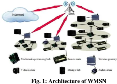
Wireless multimedia Sensor Networks (WMSNs) form a special group of WSNs and need new designs and techniques to master their challenges. WMSNs consists of a set of heterogeneous (both sensor nodes and audio video sensors (AVS)) that are connected with a base station or a sink. Base station either request the sensor nodes to transmit the sensed data or the sensor node itself can transmit the sensed data to the base station. AVS performs the sensing and processing operations and sends the data to the base station or sink. Base station collects sensed data from all the sensor nodes, process the data and sends the data to the requested user through an Internet. The WMSN architecture is presented in the Figure 1.

Fig. 1: Architecture of WMSN

Multimedia data communications can bring significant challenges to meet the requirements of Quality of Service and

Revised Version Manuscript Received on 05 August, 2019.

T Venkata Naga Jayudu, Researcch Scholar, Department of Computer Science and Engineering, JNTUA, Anantapur, Andhra Pradesh, India

M Rama Krishna Reddy, Electrical and Electronics Engineering Department, GOVT. Polytechnic, Narpala, Andhra Pradesh, India.

C Shoba Bindu, Department of Computer Science and Engineering, JNTUA, Anantapur, Andhra Pradesh, India

energy consumption. Multimedia nodes need to monitor the entire application area depending on the type of application. Nodes can consume it’s energy on performing the sensing,data processing and data transmission operations. Most of the energy can be consumed for data transmission and data forwarding from source to static sink.

Data forwarding with less energy consumption needs an efficient routing algorithm. The responsibility of routing algorithm is finding an optimized path from the sensing node to the static sink and also it is a vice versa in case of a request from static sink to the selected node. It is playing a predominant role in the research area of multimedia data communication algorithms and protocols for WMSNs. In wireless sensor networks field, many routing algorithms were proposed to deal the routing issues and energy issues. In WMSNs also some routing algorithms were proposed to solve routing problems and to fulfil the gap of such issues. The routing mechanisms and algorithms proposed in the literature were employ well known ad hoc routing issues, as well as, tactics special to wireless sensor networks, such as processing the data, employing data aggregation, clustering of nodes, heterogeneity of nodes and data-centric methods to minimize the energy consumption.

The quality of a WMSN application depends not only on how well it has been designed and implemented but also on how well it can deal with problems and events at run time. Typically WMSNs can operate in static and dynamic environments. In case of dynamic environments sensor nodes can operate with or without a human intervention. Therefore such networks should be energy aware, energy efficient and reliable to tolerate the several issues like node failure, data forwarding failure and selection of most promising neighbour to forward the data etc.

II. RELATED WORK

WMSNs can sense and transfer both scalar and multimedia data. Multimedia data contains image, audio, and video streams. The processing of multimedia data can occur in in real-time as well as nonreal-time depends on the type of application. These networks are termed as very powerful distributed systems[1]. A survey [2] presents various applications of WMSNs includes traffic avoidance, enforcement and control systems, multimedia surveillance networks, industrial process control, environment monitoring, and so forth. Most Greedy routing algorithms and techniques have been discussed[3, 4]. Mainly Greedy routing techniques considered parameters like progress,

Greedy Knapsack Based Energy Efficient

Routing in WMSNS

distance, and the direction to find the path. The first progress based routing called most forward within radius (MFR) is introduced by [5], in which the next forwarding node can be selected on the basis of maximum forward progress. In [6] authors proposed a new progress approach called nearest with forward progress (NFP), where, the next forwarder is selected with forward progress that is a node nearest to the sender. In [7,8] used direction parameter to select the next forwarder and proposed a Compass routing (DIR), which is the direction based routing. In DIR, a neighbour node which is closest to the direction of destination is selected as the next forwarder. In [9], a variant of distance based routing is proposed called Geographical distance routing (GEDIR). A DijkstraâA˘ Zs routing algorithm has been proposed to obtain the´ shortest path between two nodes in [10].

A sleep-scheduling technique is proposed and named it [11] a Virtual backbone scheduling (VBS). In this backbone sensors are responsible to forward the data and other sensors are in a sleeping mode. With this the network life time is increased. In paper [12], the residual energy and density are used to form the clusters. In this the load can be balanced among the sensor nodes by using a load balanced clustering algorithm, which can improved the network life time. A multi-path path vacant ratio and load balancing algorithm are proposed in [13], to evaluate a set of link-disjoint paths and to adjust the load. The load can be divided into segments by using threshold sharing algorithm and forwards these segments through multiple paths towards the destination. To improve the life time of wireless sensor networks, a FAF-EBRM is proposed in [14] and the selection of next forwarder is based on link weight and forward energy density to balance the energy consumption of a network. An optimal-distance-based routing scheme is proposed in the paper [15] to maximize the lifetime of the WSN, using ant colony optimization (ACO). The paper [16] maximized the life time of a network through energy balancing.

In [17],explained the importance of mobility patterns, categories of mobility patterns and how they collect the data from sensor nodes to improve the network life time. A data collection scheme named maximum amount shortest path (MASP)is proposed [18] by using controlled mobility to improve the network lifetime. And also the mobile element scheduling(MES) is used to plan a path to collect the data from the nodes. In [19] mobile element can collect the data from a set of rendezvous points (RPs), these RPs can buffer the data from the static sensors. In [20] mobile collector path planning (MCPP) and data gathering approach is proposed for a mobile collector to find the optimal path to the sojourn points(SPs) and to collect the data from those SPs. In [21],to minimize the energy consumption of a nodes proposed a Weighted Rendezvous Planning (WRP) by finding a path of a sink node. A cluster-based (CB) approach is presented to select RPs in [22] by using a binary search procedure. In [24] presented a power consumption model to calculate lifetime of motes under different event intervals.

In this work, we proposed greedy knapsack based energy efficient routing algorithm (GKEERA) to balance the energy while forwarding the data from source to sink. TIOMS is also used to provide power and to collect the data from the about to battery-drain sensor node.

III. GREEDY KNAPSACK BASED ENERGY EFFICIENT ROUTING

Energy is one of the important and limited resource in a sensor node. Every sensor node has to manage the energy in an efficient way to transmit the data from one node to another node towards the static sink with very less energy requirement. As per the proposed algorithm, assume that initially all the audio-video sensor nodes are sleep state. Whenever an event occurs in the application area, the scalar sensor nodes can triggers or activates the audio-video sensor(AVS) nodes, then AVS nodes can starts sense and captures the event details.

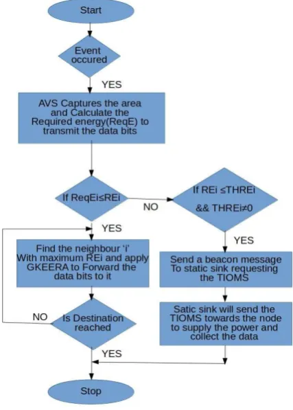
The Figure2 can explains the process of proposed work. AVS can calculates the required energy (ReqEi) to transmit the data to the neighbour. The AVS node can also requests the neighbour nodes to send their residual energy(REi’s. The AVS can select the neighbour node whose residual energy is greater than or equal to required energy, then forwards the data to that node. This procedure continues until the completion of the data transfer. Otherwise, it applies greedy knapsack based energy efficient routing algorithm (GKEERA) to divide the data with respect to the individual REi’s and forwards the data to multiple nodes.

Fig. 2: Process of proposed work

3.1Network Model

A Wireless Multimedia Sensor Networks (WMSN) is consists of scalar sensors(SS), audio-video sensors(AVS) and Two-In-One Mobile Sink (TIOMS). All these nodes uniformly distributed in a pre-defined application area except TIOMS. TIOMS is a combination of a power supplier to supply the power to requested node and a mobile sink to collect the data from that sensor node. Whenever a node’s residual energy is less than the threshold energy can send a beacon message to the static sink. Upon receiving a beacon message from a node, static sink can activates a TIOMS. Then TIOMS starts its journey to the requested node to supply the power.

We consider the following assumptions in our network model to improve the life time of a network:

1. SS and AVS nodes deployed randomly in an application area.

2. Location co-ordinates of SS and AVS are known priori.

3.Each deployed node has to send it’s residual energy to

the requested node.

4. TIOMS can supply the power and collects the data from the requested node.

5. TIOMS is aware of the location of each sensor node. 6.The TIOMS follow the shortest path to reach the requested node with in time.

3.2 Energy Model

The main energy consumption operations of a sensor node is sensing, processing, transmitting and reception of the data. Among these operations data transmission and reception operations consumes more energy compared to the sensing and processing the data. Therefore we only consider the data transmission and reception operations in our work to balance the energy in an efficiently way. Assume that a sensor node transmits one packet with K bits to the most promising neighbour node and the distance between the two nodes is D, then the energy consumption or required energy of transmission module can be presented as [23].

The proposed energy model is present in three levels: 1) node level energy model, 2) data forwarding level energy model and 3) network level energy model.

3.2.1 Node Level Energy Model:

In this we assumed that each node ’i’ has some initial energy(IEi), residual energy(REi), Threshold energy(THREi) and transmission & reception energy(TREi). Each node ’i’ either SS or AVS can calculate the ReqEi to transmit ’K’ data bits over a distance ’D’ to the most promising neighbour node. Both Energy consumption or required energy for transmission and required energy for reception is given as per the [21] is

ETX(K,D) = Eelec ∗ K + eamp ∗ K ∗ D2 (1)

ETX(K,D) is energy required for transmitting the data from

a source node to its neighbour node and Eelec is the energy required by radiating circuit and receiving circuit. Where eamp is a transmitting amplifier. Similarly, the required energy for receiving the data from the neighbour node is ERX(K,D) can be expressed as [21] :

ERX(K,D) = Eelec ∗ K (2)

The total energy required for both transmission and reception modules is shown as equation 3.

TREi = ETX + ERX (3)

ReqEi = ETX (4)

Where, ReqEi is required energy to transmit the K data bits. After every transmission the value of residual energy is updated by equation 5.

REi = IEi − ReqEi (5)

The node’s energy consumption (NEC) spent only for all the transmissions and receptions in a given time interval is expressed as:

NECi = ∑ (6)

where n is the total transmissions and Individual node’s performance can be analysed by calculating the NEC of a node.

3.2.2 Data Forwarding Level Energy Model:

Whenever a node receives a K data bits and it can calculate the required energy for transmitting these data bits. Based on the ReqEi, it can select the neighbour with maximum REi. For this it can send beacon messages to its neighbours requesting to send their residual energy in order to select the most promising neighbour to forward the data bits to that node. The algorithm 1 explains in detail about the data forwarding.

Algorithm 1 Algorithm for Data Forwarding Input: K Data bits

Output: slecting neighbour, forwarding to neighbour 1: Compute required energy ReqEi to transmit K data bits 2: Forward a beacon message bm to all its neighbours requesting to send their residual energy (REi)

3: Upon receiving a bm , all the neighbours send their REi back to the sender

4: If (ReqEi ≤ Max(REi)) then select the neighbour node with maximum RE and forward the data to that node.

5: Otherwise,apply greedy knapsack energy efficient routing algorithm (GKEERA) to forward the data bits.

6: If neighbour node is not a destination go to step 2. Otherwise data is successfully forwarded to the static sink.

Each forwarding node repeats the above algorithm 1 to forward the data bits to reach the destination. For each neighbour i, suppose a fraction Xi, 0≤ Xi ≤ 1 can be considered in to the forwarding knapsack set. This set contains the neighbours list, which have satisfied the greedy knapsack condition. Based on the residual energy of individual nodes in the set can divides the K data bits into the ratio of Xi values. The following algorithm 2 explains how a node divides the data and forwards the data in multiple paths towards the static sink.

Algorithm 2 GKEERA Input: NREi,CReqE.

Output: Forwarding knapsack set, Ki

1: Sort the received neighbour’s residual energy (NREi) in decreasing order

2: Let CReqE be current required energy

3: Choose NREi from the head of the unselected list 4: If (CReqE ≥ NREi) then {

Consider neighbour i in the forwarding knapsack set go to step 3.

} else {

Xi= CReqE/ NREi;

Consider neighbour into the forwarding knapsack set }

5: Select list of neighbours from the forwarding knapsack set, whose Xi > 0;

6: Calculate sum of required energy, SReqE=Sum(NREi*Xi);

7: If (ReqE ≤ SReqE) then { Calculate I= K / SReqE;

Divide the K data bits into k1,k2,....kn parts; Ki= I*NREi*Xi;

}

8: Forward Ki data bits to the respective neighbours. A sensor node can generate a forwarding knapsack set and divides the K data bits into the Kn parts depending on the number of nodes, which are present in the set. From equation 1, where K is directly proportional to the required energy, so we divide the K data bits into respective parts by using the algorithm 2. Then forwarding those data parts to the respective neighbour nodes, so that neighbours can follow the same procedure.

3.2.3 Network Level Energy Model:

Network level energy analysis is useful to predict the life time of a network. Total energy required to transmit the K data bits from source to destination of path length l is shown in the equation 7.

∑ ∗ ∗ (7) Where as, D is the distance between two adjacent nodes

and r is a path loss exponent. Static sink can calculate Over all network energy consumption (NWEC) by using all transmissions total energies (TotalEi) from source to sink and

it can varies in a given time interval.

∑ (8) Where n is the number of transmissions and receptions. A static sink can also find the current Network’s Residual Energy(NWRE) by using the following equation.

∑ (9) The static sink can send the bitmap to all the nodes in a predefined path, which covers all the nodes in the application area. And assume that a bitmap consumes negligible energy. The following algorithm 3 explains how to calculate the network residual energy or life time of a network.

Algorithm 3 Algorithm for Calculating Network Life Time Input: K Data bits,ReqEi Output: NWRE.

1: Static sink sends a bitmap beacon message to all the nodes requesting to insert their residual energy in the bitmap. 2: Each node can insert its REi and forwards to the neighbour.

3: Last node in that path can transmit the bitmap in a shortest path to the static sink

4: Static sink can calculate the overall residual energy of the network.

5: If NWRE ≤ NWTHRE then static sink can take necessary actions like sending TIOMS to supply power to the nodes whose RE is lessthan their threshold energy (THREi).

From the algorithm 3, static sink can be able to find the current network’s residual energy or network lifetime. Whenever static sink finds that the network lifetime is below the threshold level then it activates the TIOMS to supply the power to the nodes, whose residual energy is very less or below the threshold energy. Then TIOMS can move in a predefined path to the respective node.

3.3 Use of Mobile Sinks

In application area scalar sensors(SS) and audio-video sensors (AVS) are deployed to monitor the area. Both sensor nodes senses the surroundings and forwards the data to the static sink and then to the base station. After continuous data transmission the sensor nodes drain their energy and unable to sense the area. To avoid this case mobile sink concept is introduced in[17]. Due to mobile sink concept the distance between sensor nodes and mobile sink can be reduced and indirectly reduces the energy consumption.

Before transmitting the data, it estimates the required energy (ReqEi) to transmit a packet to the static sink and checks whether required energy is greater than residual energy(REi) of it. The node can sends a beacon message to the static sink requesting a TIOMS to supply the power and collect the data from that node. Finally we can say that the TIOMS efficiently handles the energy imbalances very easily.

V. RESULTS & DISCUSSIONS

In this section, network lifetime and energy consumption under varying parameters are presented. Further, extensive experiments are conducted to evaluate the performance of the proposed algorithm using network simulator2 (NS2) platform.

Energy efficiency analysis is done by comparing with existing routing algorithms such as WRP, CB and MCPP[20]. The parameters used in our simulation are furnished in the below table 1.

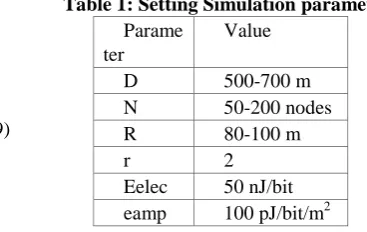
Table 1: Setting Simulation parameters Parame

ter

Value

D 500-700 m

N 50-200 nodes

R 80-100 m

r 2

Eelec 50 nJ/bit eamp 100 pJ/bit/m2

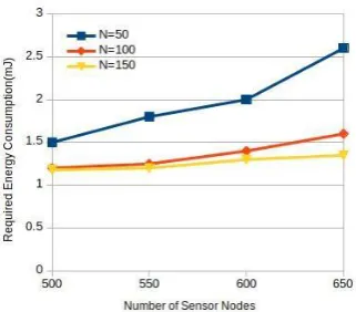
Fig. 3: Number of sensor nodes Vs Required energy consumption

Figure 3, represents required energy consumption on various sizes of the network. However, energy of 1.2 mJ is required or consumed at the network size of 500 nodes.

Fig. 4: Number of nodes Vs Network energy consumption

From figure 4, network energy consumption is increased with respect to increase in number of sensor nodes. At the network size of 50,100,150 and 200 the corresponding network energy consumptions are 18 J, 25 J,50 J and 95 J respectively. GKEERA consumes only 18 Jouls with the network size of 50 nodes and consumes 95 Jouls with the network size of 200 nodes. As compared to other methods, GKEERA consumes less energy at all sizes of the network.

Improving the network lifetime is very important challenge in WMSN. In this view, GKEERA improves the network lifetime at the network size of 50,100,150 and 200. At the network size of 200

Fig. 5: Number of nodes Vs Network life time

Fig. 6: Number of Transmissions Vs Average Energy Consumption

nodes the network lifetime with GKEERA is 4000 seconds, which is shown in figure 5. GKEERA achieves the reasonable network lifetime compared to other methods.

Figure 6 can explains, how the node’s average energy consumption can be varied with number of transmissions. After 10 transmissions GKEERA consumes only 39 Jouls.

A sensor node can prepare the knapsack forwarding set based on the GKEERA. For example, the required energy to transmit the data bits of 1000 is 1mJ. The neighbour’s residual energy is less than 1mJ, then node can create a set of forwarding nodes which satisfies the conditions present in GKEERA.

Assume that residual energies of neighbour nodes are 0.5mJ, 04mJ and 0.3mJ. GKEERA can construct the data forwarding set of nodes i.e. {n1,n2,n3} and corresponding knapsacks fractional values {1,1,0.333}. Then the corresponding node can divide the 1000 data bits into three parts like 500, 400 and 100 bits based on the knapsack set values. These data bits can be forwarded to the respective neighbour nodes. This procedure can continues until reaching the static sink. The division takes only O(n) time.

VI.CONCLUSION

GKEERA provides better performance compared to existing routing algorithms in terms of energy efficiency. It also extends the network lifetime of a wireless multimedia sensor network. Our simulation results shows that GKEERA is effective one. In future we strongly address the data aggregation in all aspects, path determination of TIOMS such that to improve the network lifetime at maximum extent. We also address the security related issues in case of misbehaving nodes.

REFERENCES

1. S. Ehsan and B. Hamdaoui. A survey on energy efficient routing techniques with QoS assurances for wireless multimedia sensor networks. IEEE Communications Surveys and Tutorials, vol. 14, no. 2, pp. 265-278, 2012. 2. I. F. Akyildiz, T. Melodia, and K. R. Chowdhury. A

survey on wireless multimedia sensor networks. Computer Networks, ScienceDirect, vol. 51, no. 4, pp. 921-960, 2007.

4. I. Stojmenovic, X. Lin. Loop-free hybrid single-path/flooding routing algorithms with guaranteed delivery for wireless networks. IEEE Trans. on Parallel and Distributed Systems,12(10),(2001),1023-1032. 5. H. Takagi, L. Kleinrock. Optimal transmission ranges for

randomly distributed packet radio terminals. IEEE Trans. on Communications, 32(3),(1984) 246-257.

6. T. C. Hou, V. O. Li. Transmission range control in multihop packet radio networks. IEEE Trans. on Communications 34(1) (1986) 38-44.

7. E. Kranakis, H. Singh, J. Urrutia. Compass routing on geometric networks. in Proc. 11 th Canadian Conference on Computational Geometry, 1999.

8. I. Stojmenovic, A. P. Ruhil, D. K. Lobiyal. Voronoi diagram and convex hull based geocasting and routing in wireless networks. Wireless communications and mobile computing 6(2) (2006) 247-258.

9. Watanabe, M., Higaki, H. (2007). No-Beacon GEDIR: Location-Based Ad-Hoc Routing with Less Communication Overhead. Fourth International Conference on Information Technology (ITNG’07), 48-55.

10. Barbehenn, Michael. (1998). A note on the complexity of Dijkstra’s algorithm for graphs with weighted vertices. Computers, IEEE Transactions on. 47. 263. 10.1109/12.663776.

11. Y. Zhao, J. Wu, F. Li and S. Lu. On Maximizing the Lifetime of Wireless Sensor Networks Using Virtual Backbone Scheduling. IEEE Transactions on Parallel and Distributed Systems, vol. 23, no. 8, pp. 1528-1535, Aug. 2012.

12. Y. Liao, H.Qi, W. Li. Load-balanced clustering algorithm with distributed self organization for wireless sensor networks. IEEE Sensors Journal13(5) (2013) 14981506. 13. S. Li, S. Zhao, X. Wang, K. Zhang, L. Li. Adaptive and

secure load-balancing routing protocol for service-oriented wireless sensor networks. IEEE Systems Journal 8(3) (2014) 858-867.

14. D. Zhang, G. Li, K. Zheng, X. Ming, Z. H. Pan. An energy-balanced routing method based on forward-aware factor for wireless sensor networks. IEEE Transactions on Industrial Informatics 10(1) (2014) 766-773.

15. X. Liu. An Optimal Distance-Based Transmission Strategy for Lifetime Maximization of Wireless Sensor Networks. IEEE Sensors Journal, 15(6) (2015) 3484-3491.

16. Z. Han, J.Wu, J. Zhang, L. Liu, K. Tian. A general self-organized tree-based energy-balance routing protocol for wireless sensor network. IEEE Transactions on Nuclear Science 61(2) (2014) 732-740.

17. Chatzigiannakis Ioannis, Kinalis Athanasios, Nikoletseas Sotiris. Sink mobility protocols for data collection in wireless sensor network. In: Proceedings of the 4th ACM international workshop on mobility management and wireless access, MobiWac’06. New York (NY, USA): ACM; 2006. p. 529.

18. Gao Shuai, Zhang Hongke, Das Sajal K. Efficient data collection in wireless sensor networks with path-constrained mobile sinks. IEEE Trans Mob Comput 2011;10(4):592-608.

19. Salarian H, Chin Kwan-Wu, Naghdy F. An energy-efficient mobile-sink path selection strategy for wireless sensor networks. IEEE Trans Veh Technol 2014;63(5):2407-19.

20. Nimisha Ghosh and Indrajit Banerjee. An energy-efficient path determination strategy for mobile data collectors in wireless sensor network. Elsevier 2015.

21. Salarian H, Chin Kwan-Wu, Naghdy F. An energy-efficient mobile-sink path selection strategy for

wireless sensor networks. IEEE Trans Veh Technol 2014;63(5):2407-19.

22. Almi ani K, Viglas A, Libman L. Energy-efficient data gathering with tour length constrained mobile elements in wireless sensor networks. In: IEEE 35th conference on Local Computer Networks (LCN), Oct 2010; 2010. p. 5829.

23. W.Heinzelman, A. Chandrakasan, H. Balakrishnan. Energy efficient communication protocol for wireless micro sensor networks, IEEE Proceedings of the 33rd International Conference on System Sciences, 2000, pp.1-10.

24. Tenager Mekonnen, Pawani Porambage, Erkki Harjula and Mika. Energy Consumption Analysis of High Quality Multi-Tier Wireless Multimedia Sensor Network, IEEE Access,Aug 2017.

ABOUT THE AUTHORS

T. Venkata Naga Jayudu, received his B.Tech degree in computer science and information technology from Jawaharlal Nehru Technological University, Hyderabad, India, in 2005. M.Tech degree in Computer Science and Engineering from Jawaharlal Nehru Technological University,Ananthapur , India, in 2011. Currently pursuing PhD in computer science at Jawaharlal Nehru Technological University, Anantapur, India. His interesting research area is wireless sensor networks, Mobile Ad-Hoc Networks, Network Security and Operating Systems.

C. Shoba Bindu, received her B.Tech Degree in Electronics & Comm. Engineering from JNTU College of Engineering, Anantapur, India, in 1997. M.Tech in Computer Science & Engineering from JNTU College of Engineering, Anantapur, India, in 2002. Received Ph.D degree in Computer Science from Jawahar Lal Nehru Technological University, Anantapur, A.P., India in May 2010. At present she is Professor in the department of Computer Science & Engg., in JNTUA, Anantapur, INDIA. Her Research Interest includes Network Security and Wireless Communication Systems, Cloud computing and Wireless networks.s