The mixed model for the analysis of a repeated‐measurement multivariate count data

DOI: 10.1002/sim.8101

R E S E A R C H A R T I C L E

The mixed model for the analysis of a

repeated-measurement multivariate count data

Ivonne Martin

Hae-Won Uh

Taniawati Supali

Makedonka Mitreva

Jeanine J. Houwing-Duistermaat

1_{Department of Mathematics,}

Parahyangan Catholic University, Bandung, Indonesia

2_{Biomedical Data Sciences, section}

Medical Statistics, Leiden University Medical Centre, Leiden, The Netherlands

3_{Department of Biostatistics and Research}

Support, UMC Utrecht, Utrecht, The Netherlands

4_{Department of Parasitology, Faculty of}

Medicine, Universitas Indonesia, Jakarta, Indonesia

5_{McDonnell Genome Institute,}

Washington University in St. Louis, St. Louis, Missouri

6_{Department of Medicine, Washington}

University in St. Louis, St. Louis, Missouri

7_{Department of Statistics, University of}

Leeds, Leeds, UK

Correspondence

Ivonne Martin, Department of Mathematics, Parahyangan Catholic University, Bandung, Indonesia; or Biomedical Data Sciences, section Medical Statistics, Leiden University Medical Centre, Leiden, The Netherlands. Email: [email protected]

Present Address

Ivonne Martin, Biomedical Data Sciences, LUMC

Funding information

Royal Netherlands Academy of Arts and Sciences (KNAW), Grant/Award Number:

Clustered overdispersed multivariate count data are challenging to model due to the presence of correlation within and between samples. Typically, the first source of correlation needs to be addressed but its quantification is of less interest. Here, we focus on the correlation between time points. In addi-tion, the effects of covariates on the multivariate counts distribution need to be assessed. To fulfill these requirements, a regression model based on the Dirichlet-multinomial distribution for association between covariates and the categorical counts is extended by using random effects to deal with the additional clustering. This model is the Dirichlet-multinomial mixed regres-sion model. Alternatively, a negative binomial regresregres-sion mixed model can be deployed where the corresponding likelihood is conditioned on the total count. It appears that these two approaches are equivalent when the total count is fixed and independent of the random effects. We consider both subject-specific and categorical-specific random effects. However, the latter has a larger computa-tional burden when the number of categories increases. Our work is motivated by microbiome data sets obtained by sequencing of the amplicon of the bacte-rial 16S rRNA gene. These data have a compositional structure and are typically overdispersed. The microbiome data set is from an epidemiological study car-ried out in a helminth-endemic area in Indonesia. The conclusions are as follows: time has no statistically significant effect on microbiome composition, the correlation between subjects is statistically significant, and treatment has a significant effect on the microbiome composition only in infected subjects who remained infected.

K E Y WO R D S

conditional model, count, Dirichlet-multinomial, generalized linear mixed model, microbiome,

multivariate, overdispersion

. . . . This is an open access article under the terms of the Creative Commons Attribution NonCommercial License, which permits use, distribution and reproduction in any medium, provided the original work is properly cited and is not used for commercial purposes.

© 2019 The Authors.Statistics in MedicinePublished by John Wiley & Sons Ltd.

57-SPIN3-JRP; MIMOmics FP7-Health-F5-2012, Grant/Award Number: 305280; Directorate General of Resources for Science Technology and Higher Education (DGRSTHE) of the Republic of Indonesia

1

I N T RO D U CT I O N

Microbiome data are overdispersed multivariate counts; for each sample, counts across multiple taxa are observed. If one

is interested in the change of the microbiome composition over time, subjects are measured longitudinally.1 _{Such data}

are subject to two sources of correlation, namely, the correlation between the counts of a sample and between multiple samples across time of a subject. For this type of data, the available statistical models are still limited.

The microbiome data set considered in this paper is obtained by sequencing the amplicon of the bacterial 16S rRNA

gene, where the sequencing procedure follows the HMP standardized protocol.2_{Chimeric sequences were filtered out and}

the resulting sequences are either categorized based on similarity into operational taxonomical units followed by annota-tion or directly annotated using relevant databases (eg, Ribosomal Database Project, Greengenes, or Silva). The counts for a specific category represent the abundances of the bacteria at a biological taxonomy level. Data sets generated through this sequencing process comprise features that have not been adequately accounted for by currently available statistical

methods.3 _{Firstly, the data set might be represented by a matrix of taxonomical counts with a compositional structure,}

which imposes a correlation between taxa.4_{Secondly, overdispersion might exist due to unobserved heterogeneity in the}

sampling procedure, the presence of taxa with rare abundance (zero-inflation), and pooling of categories. Another source might be differences in total sequence reads per sample, which might be caused by technical difficulties or by sampling or individual variability. This is commonly addressed by dividing the bacteria for each categories with the total count of the smallest reads (normalization), which results in a constant total bacterial count for all samples. Alternatively, an offset can be used in the model.

Our work is motivated by the microbiome measurements from an epidemiological study carried out in a helminth

endemic rural area in Indonesia.5_{The primary research question of this study is to analyze the joint effect of helminth}

infections and albendazole treatment on the microbial composition comprising multiple bacterial taxa. It has been hypothesized that the presence of helminths is linked with the microbial dysbiosis. However, recent findings report

incon-sistencies, probably due to limitation in the study design.1,6,7_{For our study, the stool samples were collected and measured}

on a subset of subjects participating in a randomized placebo-controlled trial. Thus, we included the microbiome data from infected subjects who received placebo, which makes our study unique. The bacterial count and the helminth infec-tion status were assessed in samples before and 21 months after the first treatment. Details of the study can be found

elsewhere.8_{In a previous paper,}5_{we identified an effect of treatment on the microbiome composition in subjects who were}

infected at baseline and at follow up. This relationship was studied in the post-treatment samples, whereas the micro-biome composition at baseline was not used. Here, we model all the available data simultaneously and hence need to address the correlation structure.

The objective of this paper is to develop a parametric model for the analysis of the overdispersed multivariate count data in the repeated-measurement setting. To date, several statistical parametric methods for analysis of microbiome data are available, which take into account the features of the data such as overdispersion and the presence of rare taxa. One approach is to consider a univariate taxa of interest and model the association of this taxa with biological covariates. Sev-eral regression models for this simplified problem exist. Zero-inflated models or hurdle models have been proposed to

deal with rare taxa.9 _{These models are also available for longitudinal studies. This approach however ignores the}

mul-tivariate structure of the data. A second approach, which considers the compositional feature of the microbiome data, models the multivariate count outcome across taxa by a multinomial distribution. To deal with overdispersion, the

under-lying parameters are assumed to follow the conjugate distribution.10_{This formulation has an advantage that the marginal}

distribution has a closed-form formula.

The correlation due to repeated-measurements within the same person is often modeled by including a normally distributed random effect in the linear predictor, ie, generalized linear mixed model. The overdispersion is typically

accounted for by the conjugate distribution.10-12_{Molenberghs et al}13,14_{and Booth et al}15 _{introduced a combined model,}

distributed random effects, ie, generalized linear mixed model. The authors only consider single categorical count data; hence, these models cannot be directly applied to our data, where we have to acknowledge the compositional feature. Therefore, in spirit of the combined model, we propose an extension of the Dirichlet-multiomial regression model with random effects to incorporate the correlation due to repeated measurements. We will use the reparameterization of

the work of Guimarães and Lindrooth,12 _{in which the overdispersion is a function of the covariates and the random}

effects.

This manuscript is organized as follows. In Section 2, we briefly describe the formulation of the loglinear model in the setting of multivariate count data and derive the likelihood of the multinomial distribution obtained by conditioning on the total count. We show the derivation of this method in the case where the count is overdispersed. The model is then extended to include the correlation due to repeated measurements over time. In Section 3, simulation studies are described to investigate the performance of the proposed methods and the results of the analyses of the motivating data set are presented in Section 4. In Section 5, we conclude and discuss the proposed method.

2

M ET H O D S

A novel mixed model is considered for the relationship between counts of six phyla categories and the binary variables of infection status and treatment allocation before and after the first treatment round. Due to the normalization, the total count per sample is fixed at 2000 at each time point. Before introducing our new model, we will review various models for categorical count data in the cross-sectional setting, namely, for independent count data (the loglinear and the multinomial logistic regression model) and for count data subject to overdispersion (the negative binomial and the

Dirichlet-multinomial model).16,17

We first introduce the following notations. LetC(_it) = {C_i(₁t),…,C_iJ(t)}be theJ-dimensional vector of the multivariate

microbial count withC(_i𝑗t)the abundance of bacteria taxaj(j = 1,…,J) for subjecti(i = 1,…,N)at time-pointt. The

total count for each subjectiat time-pointtis fixed and denoted asC(_i+t) = ∑J_𝑗=1C(_it_𝑗). LetPbe the number of categorical

covariates andX_i(t) be theP-dimensional vector of covariate values for subjectiat time-pointt. When modeling

micro-biome data as described earlier, either the sequence count itself can be considered or the normalized count related to the total sequence read, ie, compositional data. Multiple counts distributed over categories are usually represented by a

contingency table. We briefly review models for the cross-sectional setting and therefore suppress the superscripttin the

model formulation in Section 2.1.

2.1

Cross-sectional setting

2.1.1

The loglinear model for two categorical variables

The loglinear model is commonly used to model the association between multivariate categorical count data and predic-tors of categorical or continuous value. In the case where all variables are categorical, the data can be represented by a

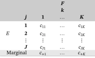
contingency table. Consider two categorical variablesEandF, withJandKlevels, respectively. The count outcomecjkis

associated with thejth level of predictorEandkth level of predictorF, which could be described in aJ× Kcontingency

table (Table 1) as follows.

Each cell's count outcomecjkis assumed to follow a Poisson distribution with a mean𝜇jk. Here, the saturated loglinear

model for such contingency table is given by

log(𝜇_𝑗k) =𝜆0+𝜆E_𝑗 +𝜆F_k +𝜆EF_𝑗k, (1)

TABLE 1 TheJ×Kcontingency table

F k

j 1 … K

1 c11 … c1K

E 2 c21 … c2K

⋮ ⋮ ⋮ ⋮

J cJ1 … cJK

where𝜆0,𝜆0+𝜆E

𝑗,𝜆0+𝜆Fk, and𝜆0+𝜆

F k+𝜆

E

𝑗 +𝜆EF𝑗k represent the overall mean, the marginal mean of categorical variable

Eat thejth level, the marginal mean of variableFat thekth level, and the mean when variablesEandFtaking the value

jandk, respectively. Because there areJ ×Kcells, theJ + K + JK + 1 parameters of the saturated loglinear model (1)

are not uniquely identifiable and, thus, constraints are needed to ensure the model identifiability. Two sets of constraints are commonly used, namely, the baseline and the symmetrical constraint, given by

𝜆E

1 =𝜆

F

1 =𝜆

EF

𝑗1 =𝜆EF1k =0

and

J

∑

𝑗=1 𝜆E

𝑗 =

K

∑

k=1 𝜆F

k = J

∑

𝑗=1 𝜆EF

𝑗1 =

K

∑

k=1 𝜆EF

1K =0, for all𝑗,k,

respectively. In this manuscript, we use the baseline constraint.

Note that, in model (1), the response (bacterial categories)Eand predictorFare exchangeable. The loglinear model (1)

could be written in the regression format for the bacterial outcome as follows:

log(𝜇𝑗k) =𝜉0𝑗+𝜉1𝑗k[F=k], 𝑗=1,…,J, k=1,…,K,

with[.]as the indicator function. To show the equivalence between two models, note that the followingjruns over the

category andkruns over the predictor levels. For a subject with their predictor in categoryk = 1, the regression model

{𝜉01, 𝜉02,…𝜉0J}with𝜉0jforj = 2,…,Jcorresponds to𝜆0+𝜆E_𝑗. For subjects with their predictor in other categoriesk,

the regression model{𝜉01 + 𝜉11k, 𝜉02 + 𝜉12k,…, 𝜉0J + 𝜉1Jk}, where𝜉1jkforj = 2,…J, corresponds to𝜆F_k+𝜆EF_𝑗k. Thus, in

the context of regression, the𝜆EF

𝑗k represents the effect of the categorical variableFon outcome categoryjrelative to the

reference category.

To estimate the parameters, we assume that each cell's entry represents a realization from the Poisson distribution. The

maximum likelihood estimate of𝝀or of𝝃can be obtained by maximizing the following likelihood function. Specifically,

for subjecti, it is given by

Li(𝝀) =

∏

𝑗

𝑓Pois(𝝀;ci𝑗k)

=∏

𝑗

exp(−𝜇_𝑗k)𝜇 ci𝑗k

𝑗k

ci𝑗k! ,

(2)

where personibelongs to categorykand has counts in each bacteria categoryj. The model could be straightforwardly

gen-eralized to incorporate more categorical covariates, which results into more than two-way contingency table. For instance, when incorporating the infection and treatment status, we will have a three-way contingency table. As previously, the

categorical variableEcorresponds to the bacteria category, variableFto the treatment randomization arm, andGto the

infection status. The corresponding loglinear model can be written as follows:

log(𝜇_𝑗kl) =𝜆0+𝜆E_𝑗 +𝜆F_k+𝜆EF_𝑗k +𝜆G_l +𝜆EG_𝑗l +𝜆FG_kl +𝜆EFG_𝑗kl , 𝑗=2,…,J;k=l=2

or in the regression format as

=𝜉0_𝑗+𝜉1_𝑗Treatment+𝜉2_𝑗Infection+𝜉3_𝑗Treatment×Infection, 𝑗=1,…,J, k=l=1,2. (3)

Here, the baseline constraint is applied on the first equation, whereas, for the second equation, this is not needed because

there are onlyJ×Pparameters. This last equation represents the loglinear model written in terms of regression coefficients

𝝃and covariate values, where Treatment and Infection are binary variables. To assess the statistical significance of the

pth covariate(p = 1,…,P)on the multivariate count distribution, the null hypothesis𝝃_p = 0should be tested. We will

use the standard likelihood ratio test, which follows a𝜒2_{distribution withJdegrees of freedom.}

2.1.2

Multinomial logistic regression

In our data example, the total bacterial count is fixed to a constant for all samples. Under this constraint of a fixed total

count, it is sufficient to model the counts forJ−1 categories and(J−1) ×Pparameters are uniquely identified. Guimarães

and Lindrooth12_{showed that the distribution of the multivariate counts under the constraint that the total is a constant}

could be derived from the distribution of the unconstrained multivariate counts earlier by using the conditional log

total countc+kl follows a Poisson distribution with mean

∑J

𝑗=1𝜇𝑗kl = 𝜇+kl. The distribution of the multivariate counts

conditional on the total for each subjectiis therefore given by

Pr(ci= {c1kl,…,cJkl}|c+kl) =

Pr(c1kl,…,cJkl,c+kl)

Pr(c+kl)

=

J

∏

𝑗=1

𝑓Pois(c_𝑗kl;𝜇𝑗kl)

𝑓Pois(c+kl;𝜇+kl)

=c+kl! J

∏

𝑗=1

( 1 c_𝑗kl!

) (_𝜇

𝑗kl

𝜇+kl

)c_𝑗kl

∼Multinomial(c+kl;𝜋1kl,…, 𝜋Jkl), where𝜋𝑗kl=

𝜇𝑗kl

𝜇+kl

. (4)

Thus, under the baseline constraint and the constraint that the total count is fixed, the distribution of the

multivari-ate count is equivalent to the multinomial distribution with parameter𝜋_𝑗 = 𝜇𝑗

𝜇+

. This model is the multinomial logistic

regression model. Note that the parameters𝝀of the loglinear model (1) cancel out. In the multinomial logistic regression

model, the parameters of the reference category are typically assumed to be equal to zero, although other constraints can be used as well.

2.1.3

Overdispersed count data

When the count data are overdispersed, the variance of the cell count is no longer equal to its expected value and the Poisson distribution cannot be used. A common approach to deal with overdispersion is to assume that the conditional

mean of the count outcome is a random variable following the conjugate distribution. Consider a count at categoryj

and let exp(𝜂i𝑗)be the random effect for overdispersion following the Gamma distribution (conjugate for Poisson) with

parameter𝜃. Guimarães and Lindrooth formulated the model for an overdispersed count outcome as follows:

Ci𝑗|exp(𝜂i𝑗) ∼Pois(𝜇̃i𝑗), 𝑗=1,…,J ̃

𝜇i𝑗=exp(𝜂i𝑗)𝜇i𝑗, where exp(𝜂i𝑗) ∼ Γ(shape=𝜃−1𝜇i𝑗,rate=𝜃−1𝜇i𝑗) ̃

𝜇i𝑗=exp(𝜂i𝑗)𝜇i𝑗∼ Γ(shape=𝜃−1𝜇i𝑗,rate=𝜃−1).

Here,𝜇ijcorresponds to the mean of the count in the nonoverdispersed model. Now, the marginal distribution for the

count at categoryjin personi,Cij, can be obtained by integrating out the random effect exp(𝜂i𝑗)as

Pr(Ci𝑗) =

∞

∫

0

Pr(Ci𝑗|exp(𝜂i𝑗))g(exp(𝜂i𝑗))dexp(𝜂i𝑗)

= Γ(𝜃

−1_𝜇

i𝑗+Ci𝑗)

Ci𝑗!Γ(𝜃−1𝜇i𝑗)

( ₁

𝜃−1₊₁

)Ci𝑗( 𝜃−1 𝜃−1₊₁

)𝜃−1_𝜇

i𝑗 .

This corresponds to a negative binomial distribution with parameters (

𝜃−1_𝜇

i𝑗, 𝜃

−1 1+𝜃−1

)

. By the properties of the negative

binomial random variable, the total count for subjectialso follows the negative binomial distribution

Ci+∼NB

(

𝜃−1_𝜇

i+, 𝜃 −1

1+𝜃−1

)

.

The likelihood for subjectiin this setting is given by

Li(𝜃,𝝀) =

∏

𝑗

𝑓NB(𝝀, 𝜃;Ci𝑗)

=∏

𝑗

Γ(𝜃−1_𝜇

i𝑗+Ci𝑗

)

Ci𝑗!Γ

(

𝜃−1𝜇

i𝑗

) (_𝜃−11

+1

)Ci𝑗( 𝜃−1 𝜃−1₊₁

)𝜃−1_𝜇

i𝑗

. (5)

Note that, in this setting, parameter𝜃, which models the overdispersion and the intercept𝜆0, is not identifiable. An

often used solution is to absorb the overdispersion parameter into the grand mean𝜆0, ie,𝜃−1_{exp(𝜆0) =𝛿}−1

2.1.4

Overdispersed multinomial

We briefly review the overdispersed count data introduced by Guimarães and Lindrooth as follows. To guarantee that the parameters of the count for each category follows a Gamma distribution with the same rate parameter, the

overdis-persion parameter exp(𝜂i𝑗)needs to be a function of the linear predictor𝜇ij. For such a distribution, theorem 1 in the

work of Mossiman18_{can be applied. This theorem states that, ifC}

i = {Ci1,Ci2,…,CiJ}are independently Gamma

dis-tributed random variables with parameters(̃𝜇i1, ̃𝜇i2,…, ̃𝜇iJ)with the same scale parameter𝜃−1, then the random variables

𝚷i = {Πi1,Πi2,…,Πi J}withΠi𝑗 = ∑JCi𝑗

𝑗=1Ci𝑗 have a multivariate beta distribution (Dirichlet distribution) with

parame-ters{̃𝜇i1, ̃𝜇i2,…, ̃𝜇iJ}. Note that the Dirichlet distribution is the conjugate for the multinomial distribution. Hence, the

marginal distribution for the random variable𝚷i is obtained by integrating out the Dirichlet random effects. Now, the

corresponding Dirichlet-multinomial distribution is given by

Pr(𝚷i) =

Γ(𝜇̃i+)Ci+!

Γ(𝜇̃i++Ci+)

J

∏

𝑗=1

Γ(𝜇̃i𝑗+Ci𝑗) Γ(𝜇̃i𝑗)Ci𝑗!

. (6)

Alternatively, we consider the conditional likelihood of the multivariate negative binomial given the total count. The

contribution for theith subject is given by

Li(𝝀, 𝜃) =Pr(Ci|Ci+) =

∏J

𝑗=1𝑓NB(Ci𝑗;𝜇̃i𝑗) 𝑓NB(Ci+;𝜇̃i+)

= Γ(𝜃

−1_𝜇

i+)Ci+!

Γ(𝜃−1𝜇

i++Ci+)

J

∏

𝑗=1 Γ(𝜃−1_𝜇

i𝑗+Ci𝑗)

Γ(𝜃−1𝜇

i𝑗)Ci𝑗! . (7)

By𝜇̃i𝑗=𝜃−1𝜇i𝑗, it follows that the likelihood (7) is equivalent to the Dirichlet-multinomial distribution (6). Here,

param-eter𝜃is unidentifiable. Similar to (5), we apply the parameterization in the work of Guimarães and Lindrooth,12_where

the overdispersion is absorbed in the grand mean𝜆0such that𝜃−1_{exp(𝜆0) =𝛿}−1

0 in the reference category. In contrast to

the nonoverdispersed multinomial model, the intercepts of the overdispersed multinomial model do not cancel out.

2.2

Repeated-measurement of overdispersed count

In addition to the overdispersion due to the presence of multiple bacteria within one sample, there is also correlation between measurements of the same person at the two time-points, ie, at the pre- and post-treatment. To deal with this

correlation, we propose to include a random effectuiin the linear predictor of the model and assume that, conditional

on this random effect, the observations of the two time points are independent. We further assume that the random

effectuifollows a normal distribution with zero mean and variance𝜎2u. The idea of using different distributions for the

random effects representing overdispersion and correlation was introduced by Molenberghs et al13,14_{and Booth et al.}15

Molenberghs and Booth modeled the mean of an outcome as a multiplication of overdispersion and the linear predictor. However, to guarantee that the theorem 1 in the work of Mossimann holds, ie, that the proportion of each bacterial category has Dirichlet-multinomial distribution, we need to model the overdispersion as a function of the linear predictor. In the rest of this section, we describe three different mixed models for multivariate count data with overdispersion in

the repeated-measurement setting using random effects, conditional on the random effectui: the counts follow the

multi-variate negative binomial distribution; the counts follow the conditional multimulti-variate negative binomial distribution given the total count; and the proportions (cell's count divided by total count) follow the Dirichlet-multinomial distribution. In

all models, we will add the random effectuito the linear predictor. These models are therefore extensions of the models

for overdispersed multivariate count given in Section 2.1. Specifically, for the first model, we assume that, conditional on the random effects exp

(

𝜂(t)

i𝑗

)

andui, the countC(_it_𝑗)follows a Poisson distribution with mean equal to

E [

C(_i𝑗t)||

||exp (

𝜂(t)

i𝑗

)

,ui

]

=exp (

𝜂(t)

i𝑗

) exp

(

̃𝜇(t)

i𝑗

)

, where𝜇̃_i(_𝑗t)=Xi𝝃𝑗+ui, 𝑗 =1,…,J.

exp (

𝜂(t)

i𝑗

)

∼ Γ

(

shape= 𝜃−1exp

(

̃ 𝜇(t)

i𝑗

)

,rate= 𝜃−1exp(Xi𝝃_𝑗+ui)

)

Thus, given the random effectui, the two vectors of countsC(_it)fort = 1 andt = 2 are independently distributed and

follow the negative binomial distribution. The corresponding likelihood can be written as follows:

LUNBM

(

𝝃, 𝜃, 𝜎2

u ) =∏ i Pr (

C(_it) ) =∏ i ∫ ui Pr (

C_i(₁t),…,C(_iJt),ui

)

d ui

=∏

i ∫ ui

2

∏

t=1

J

∏

𝑗=1

Pr (

C(_i𝑗t)|ui

)

Pr(ui)d ui, (9)

and we denote the regression model under this likelihood to be the unconstrained negative-binomial mixed model (UNBM).

For the second approach, we consider the counts following the conditional multivariate distribution given the total count. When each categorical count conditional on the total count follows the negative binomial

with the same rate parameter, the total count C(_it₊)|ui follows the negative binomial distribution with parameters

(∑J

𝑗=1exp

(

𝜂(t)

i𝑗

) exp

(

̃ 𝜇(t)

i𝑗

)

, 𝜃−1 1+𝜃−1

)

. Thus, the corresponding conditional likelihood is given by

LCNBM

(

𝝃, 𝜃, 𝜎2

u ) =∏ i Pr (

C(_i1),C(_i2)||_|C(_i+1),C_i(₊2)

)

=∏_i

∫_u

iPr (

C_i(1),C_i(2),C(_i1) +,C

(2)

i+|||ui

)

Pr(ui)d ui

∫_uiPr (

C(_i+1),C(_i+2),ui

)

d ui

=∏_i

∫_u

i ∏2

t=1

∏2 𝑗=1Pr

(

C(_i𝑗t)||_|ui

)

Pr(ui)d ui

∫_u

i ∏2

t=1Pr

(

C(_it) +|||ui

)

Pr(ui)d ui

. (10)

The model corresponding to this likelihood is denoted as the conditional negative-binomial mixed model (CNBM).

How-ever, when the total counts depends onui, the total count should be a random variable. This is not the case in our data

set. Therefore, we propose the third method with the assumption that the total count is independent ofui.

In the third approach, we model the multivariate counts in terms of the relative abundance. We assume that the vector

of proportionsΠ(_it)conditional on the random effectuifollows the Dirichlet multinomial distribution, ie,

{

C(_i1t) C(_i+t),…,

C_i(₁t) C_i(₊t)

}| || || |

{

𝛼(t)

i1,…, 𝛼 (t)

i𝑗

}

,ui∼Mult

(

̃𝜋(t)

i1,…, ̃𝜋 (t)

iJ

)

{

̃𝜋(t)

i1,…, ̃𝜋 (t)

iJ

}

∼Dir (

𝛼(t)

i1,…, 𝛼 (t)

iJ

)

𝛼(t)

i𝑗 =𝜃−1𝜇 (t)

i𝑗, (11)

where𝜇(_i𝑗t)is the linear predictor as in the loglinear model for the Poisson count. With this parameterization, the expected

multinomial parameter becomes

̃ 𝜋(t)

i𝑗 =

exp (

𝜂(t)

i𝑗

) exp

(

̃ 𝜇(t)

i𝑗

)

∑J

𝑗=1exp

(

𝜂(t)

i𝑗

) exp

(

̃ 𝜇(t)

i𝑗

).

The likelihood for each subjectiis then formulated as follows:

LDMM

(

𝝃, 𝜃, 𝜎2

u

)

=Pr (

C(_i1)

C(_i+1),

C(_i2)

C(_i2₊)

)

=_∫

ui Pr

( C(_i1)

C(_i1₊),

C(_i2)

C(_i+2)

|| || ||ui

)

Pr(ui)d ui

=

∫

ui

2

∏

t=1 Γ

(

𝜃−1_𝜇(t)

i+

)

C(_it₊)! Γ

(

𝜃−1𝜇(t)

i++C (t)

i+

)

J

∏

𝑗=1 Γ

(

𝜃−1_𝜇(t)

i𝑗C

(t)

i𝑗

)

Γ

(

𝜃−1𝜇(t)

i𝑗

)

C_i(_𝑗t)!

Pr(ui)d ui. (12)

The corresponding regression model under this likelihood is denoted as the Dirichlet-multinomial mixed model (DMM).

It is shown in Appendix A that, in the case where the total count does not depend on the random effectui, the likelihoods

(10) and (12) are equivalent.

The variance of the random effectu(𝜎2

u) represents the correlation between the samples of the same subject across time.

interesting. This correlation is given by

Corr (

Ci𝑗(t),C(t

∗₎

i𝑗∗ )

= 𝜎_Ci

𝑗(t),C(i𝑗t∗ )∗ √

𝜎2

C(t) i𝑗

·𝜎2

C_i(_𝑗t(∗) )∗

.

The marginal correlation can be computed from Monte-Carlo estimates of the first and second moments.

The program language R is used for all the computations except for data application with categorical-specific random effects. When maximizing the likelihoods, the integrals are approximated by the adaptive Gauss-Hermite quadrature

method,19_{and we used the functions available in the ecoreg package}20_{to compute the integral. R implementations are}

available in github (https://github.com/IvonneMartin/CombinedMultinomial).

2.3

The categorical-specific random effect

In the aforementioned parameterization, we assume that the subject-specific effectuiis univariate and is the same for

all bacteria categories and time points. Alternatively, aJ-dimensional vector of random effects can be used. Equation (8)

now becomes

̃ 𝜇(t)

i𝑗 =Xi𝝃_𝑗+ui𝑗, 𝑗 =1,…,J.

ui𝑗∼MVN(𝟎,ΔJ×J). (13)

Here, each bacterial category has its own realization of the random effect and the random effects solely model

corre-lation between the categories over time. The vectoruiof lengthJfollows a multivariate normal distribution with aJby

Jdiagonal variance matrixΔwith𝜎2

𝑗 as diagonal elements. In addition to the general model (13), we consider a model

with common variance𝜎2

𝑗 = 𝜎u2, for allj, to reduce the parameter space. Since the overdispersion already takes care of

the correlation among the categories, this model might be better interpretable. However, a drawback of this model is that

computation of the likelihood function involves an intractableJ-dimensional integral.

3

S I M U L AT I O N ST U DY

3.1

Simulation setting

Three sets of simulation studies were conducted to evaluate the performance of the proposed methods. With regard to estimation of the fixed effect parameters and variance components, we first investigated the performance of the DMM models for a subject- and categorical-specific random effects. We reported the bias and MSE as well as the sensitivity and specificity for these parameters. The sensitivity and the specificity of the likelihood ratio test statistics were computed for the following pairs of hypotheses (for fixed and variance of random effect, respectively):

H0∶𝝃p=𝟎 vs H1∶at least one of 𝝃p ≠0,

H0∶𝜎u2=0 vs H1∶𝜎u2>0.

In the second set, we want to estimate the marginal correlation given the distribution of the random effect. The purpose of this study is to verify whether the marginal intraclass correlation observed in our motivating data set can be represented by our models (UNBM and DMM). For this purpose, we vary the standard deviation of the random effect and we used 10 000 Monte-Carlo simulation for estimating the marginal intraclass correlation.

In the third set, we aimed to study the robustness of the parameter estimates by fitting the DMM models when the true model is UNBM. For this purpose, we generated data sets with three categories from the UNBM model.

3.1.1

Data set generation

To reduce the computational burden, data sets with only three categories at two different time-pointstwere considered.

The total count per sampleSwas 25, 50, or 2000, and the number of samplesNwas 150 or 500. Two sets of parameters

were used, namely,𝝀was fixed at{𝜆F₂, 𝜆₂E, 𝜆E₃, 𝜆EF₂₂, 𝜆EF₃₂} = {0.5,−1,0.1,0.8,−2}as well as the parameters from the data

set (results are given in Supporting Information Table S1). To increase the power, the parameter values of the first set are

The overdispersion parameter was fixed at𝜃 = 0.1. For the standard deviation of the random effects, we considered

values𝜎uof 0.5, 0.8, and 1.

Specifically, for the Dirichlet-multinomial mixed (DMM) model with a univariate random effect, multivariate counts were generated as follows.

1. For each subjecti,i = 1,…,N, we randomly generate binary covariatesXt

i for each time-pointtand a random effect

ui∼N(0, 𝜎u2).

2. The mean for each categoryjis computed as ̃𝜇_i(_𝑗t) =𝜃−1_exp(𝝀+u

i), where𝝀correspond to𝜉.

3. A multivariate count with mean ̃𝜇(_i𝑗t)is generated.

For the DMM model with multivariate random effect, a similar procedure was used except that the random effects in

step (1) are now generated from the multivariate normal distribution with a diagonal covariance matrixΣ. We considered

three sets of values for the standard deviations of random effects, namely,𝝈u= (𝜎u1, 𝜎u2, 𝜎u3)is (0.5,0.6,0.5), (0.8,0.9,0.8),

or (1,0.9,1).

For the second set of simulation, six bacterial categories are used and parameters for the simulation are obtained from the data set. Finally, for the unconstrained negative binomial mixed (UNBM) model, the second step was replaced by

computation of the expected count outcome for each categoryjof𝜇̃i𝑗 = 𝜃−1exp(log(S) +𝝀+ui). Here, the offset log(S)

is incorporated to take into account the total bacteria countS. For each scenario mentioned earlier, 1000 replicates were

generated. The models were fitted to each of the replicates.

3.2

Simulation results

3.2.1

Evaluation of DMM model

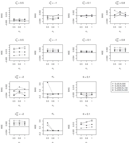
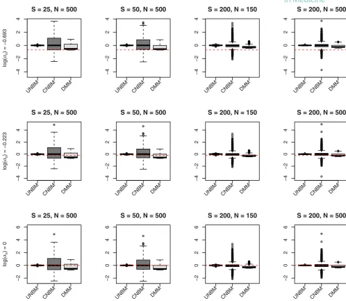
The performance of the method in estimating the parameters is described in Figure 1. Overall, the bias and MSE appear

to be improved when either the total bacterial count (fromS = 25 toS = 50 and the sample size wasN = 500) or the

sample size was increased (fromN = 150 toN = 500 and the total count wasS = 2000). For a small value of𝜎u, both the

bias and the MSE of this estimate are relatively large. Similar results are obtained for the model with categorical-specific random effects (Figure S1). The sensitivity of the likelihood ratio test for the fixed effects parameters that are obtained from the data set are very low for all scenarios except when the total sample size is large (Table S2A). For testing the zero variance component, the likelihood ratio test has a high sensitivity and specifity when the sample size and variance component are large (Table S2B).

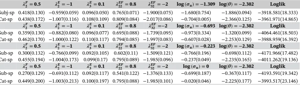
Since the model with the categorical-specific random effect is time consuming to fit, we also investigate the robustness of assuming a subject-specific random effect, whereas the data sets were generated by using a vector of random effects following the multivariate normal distribution. The results are given in Table 2. It appears that, for a random effect with

smaller standard deviation (log(𝜎u)of−1.309), the biases of the estimates of fixed effect parameters and of log(𝜎u)are

relatively small, whereas, for a random effect with larger standard deviation log(𝜎u) =0 (𝜎uof 1), the biases are relatively

large.

In Table S3, the marginal correlations are given for the subject-specific random effects. It appears that the correlation between categories are all negative and the correlation between samples across time are very small. These results are not affected by the standard deviation of the random effect for our considered values. Table S4 lists the marginal correlations using categorical-specific random effects, where each category-specific random effect has the same standard deviations

𝜎u. We notice that a part of the correlations between categories is now positive and the correlation between the same

categories across time is larger. Moreover, these correlations tend to increase with a larger variance of the random effects.

3.2.2

Simulations under the UNBM model

The marginal correlations for the UNBM with a subject-specific random effect are listed in Table S5. It appears that the correlations between categories are positive as well as negative. The correlations of the same category between time points

are all positive and increase with𝜎u. A similar result is observed for the UNBM model with categorical-specific random

effects (Table S6) although, here, the correlation varies more across categories.

FIGURE 1 Bias and mean squared error (MSE) of data sets generated from the Dirichlet-multinomial mixed model with subject-specific random effect.𝝀: a vector of parameters in loglinear model.𝜎u: the standard deviation of the between individual variation.𝜃the overdispersion

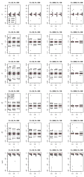
(CNBM), and the Dirichlet-multinomial mixed model (DMM) are given in Figure 2 for the fixed effect parameters and Figure 3 for the variance component.

In general, the fixed effect parameters obtained from these three different models are unbiased except the estimates

of the intercepts (𝜆F₂) for the CNBM model and the DMM model. Since the model used for analysis and generating the

data are the same, the estimates of the fixed effect parameters in Figure 2 are unbiased and the variance of the estimator

TABLE 2 The mean estimates (standard deviation) over 1000 replicates when data sets were generated from the Dirichlet-multinomial mixed model with categorical-specific random effect with common variance

𝝀F

𝟐 =0.5 𝝀E𝟐 = −1 𝝀E𝟑 =0.1 𝝀EF𝟐𝟐 =0.8 𝝀EF𝟑𝟐 = −2 log(𝝈u) = −1.309 log(𝜽) = −2.302 Loglik

Subj-sp 0.418(0.130) −0.959(0.059) 0.096(0.050) 0.765(0.071) −1.900(0.075) −1.680(0.754) −1.886(0.094) −3918.581(18.333) Cat-sp 0.438(0.172) −1.007(0.116) 0.108(0.109) 0.809(0.084) −2.017(0.086) −0.704(0.005) −2.366(0.125) −3961.971(14.865)

𝝀F

𝟐 =0.5 𝝀E𝟐 = −1 𝝀E𝟑 =0.1 𝝀EF𝟐𝟐 =0.8 𝝀EF𝟑𝟐 =−2 log(𝝈u) = −0.693 log(𝜽) = −2.302 Loglik

Sub-sp 0.359(0.130) −0.882(0.080) 0.096(0.077) 0.695(0.088) −1.739(0.095) −0.973(0.334) −1.320(0.099) −4064.461(18.503) Cat-sp 0.462(0.170) −1.000(0.122) 0.110(0.117) 0.794(0.085) −1.997(0.083) −0.607(0.028) −2.253(0.129) −3988.959(16.392)

𝝀F

𝟐 =0.5 𝝀E𝟐 = −1 𝝀E𝟑 =0.1 𝝀EF𝟐𝟐 =0.8 𝝀EF𝟑𝟐 = −2 log(𝝈u) = −0.223 log(𝜽) = −2.302 Loglik

Sub-sp 0.300(0.132) −0.766(0.099) 0.092(0.105) 0.602(0.11) −1.509(0.121) −0.766(0.196) −0.698(0.112) −4171.966(17.482) Cat-sp 0.455(0.194) −1.004(0.173) 0.099(0.17) 0.795(0.089) −1.985(0.096) −0.237(0.049) −2.235(0.165) −4011.262(19.136)

𝝀F

𝟐 =0.5 𝝀E𝟐 = −1 𝝀E𝟑 =0.1 𝝀EF𝟐𝟐 =0.8 𝝀EF𝟑𝟐 = −2 log(𝝈u) =0 log(𝜽) = −2.302 Loglik

Sub-sp 0.270(0.129) −0.691(0.112) 0.092(0.117) 0.541(0.122) −1.376(0.133) −0.699(0.187) −0.367(0.117) −4193.591(19.342) Cat-sp 0.449(0.200) −1.003(0.213) 0.100(0.197) 0.795(0.088) −1.985(0.101) −0.020(0.046) −2.225(0.177) −3993.517(23.146)

Each rows started with Sub-sp represents the estimates (standard deviation) when data sets were fitted with the DMM model with subject-specific random effect and rows started with Cat-sp represents the estimates (standard deviation) when data sets were fitted with DMM model with categorical-specific random effect having common variance.

𝝀, 𝜎u, 𝜃are as explained in Figure 1.

Loglik represents the loglikelihood value obtained using the corresponding model.

Rows in gray represent the estimation when the standard deviation of the normally distributed random effect is small.

toN = 500). When using the conditional distribution, given the total, the estimates of the fixed effect parameters in

Figure 2 are biased when the total bacterial count is small (S = 25 andS = 50). When the total count is relatively large

(S = 2000), the estimates of the fixed effects (including the intercept𝜆F

2) are less biased. When estimating the fixed effect

parameters using the DMM model, the estimate of the fixed effects are unbiased except for the intercept term𝜆F

2 and

increasing the sample size does not improve the estimation.

The estimates of the random effect parameters in the UNBM model are unbiased and, by increasing the total bacterial

count or the sample size, improve the precision. In the CNBM model, when the total bacterial count is small (S = 25

andS = 50), we observe that the standard deviation ofui is overestimated and that the bias in the estimate of the

overdispersion parameter is small. When the total count is largeS = 2000, the estimate of the standard deviation ofui

appears to be less biased, whereas the overdispersion parameters are underestimated. When fitting the DMM model to the data, the estimates of the random effect parameters are biased in all scenarios.

4

DATA A P P L I C AT I O N

We used the DMM models to analyze the effect of helminth infections and treatment on microbiome composition. For this purpose, we first consider the fixed effect structure and fitted several DMM models to our data set assuming (common) random effect for each category. Next, we will investigate the best random effect structure and we will verify whether the parameter estimates of the fixed effects are affected by the random effect structure.

The microbiome data set considered here was measured in a subset of a randomized clinical trial performed in

a helminth-endemic area in Nangapanda subdistrict, Indonesia, described elsewhere8 _{and is publicly available at}

Nematode.net (http://nematode.net/Data/Indonesia_16S/S1_Table.xlsx). In brief, households were randomized to receive either a single dose of 400 mg albendazole or placebo, once every three months for a period of one and a half years. To assess the effect of treatment on the prevalence of soil transmitted helminth infections, yearly stool samples were

col-lected on a voluntary basis.T. trichiurainfection was detected by microscopy and a multiplex real-time PCR was used to

detect the DNA of hookworm (Ancylostoma duodenaleorNecator americanus) andAscaris lumbricoides. A subject was

regarded as infected if it was infected with at least one helminth species.

For the current study, paired DNA samples before and at 21 months after the first treatment round from 150 inhabitants in Nangapanda were selected based on the treatment allocation and infection status, as well as the avail-ability of complete stool data at pre- and post-treatment. The procedure for sample collection and processing was

already described in the work of Wiria et al.8 _{The 16s rRNA gene from the stool samples was processed through}

the 454 pyrosequencing technique, and the classification of the sequence resulted in counts of 18 bacterial phyla. For the current analyses, we retained the five most prevalent phyla and pooled the remaining into one category,

resulting in six phyla categories: Actinobacteria, Bacteroidetes, Firmicutes, Proteobacteria, unclassified, and pooled

−4

−2

0

2

4

S = 25, N = 500

log(

) = −0.693

UNBM CNBM DMM

−4

−2

0

2

4

S = 50, N = 500

UNBM CNBM DMM

−4

−2

0

2

4

S = 200, N = 150

UNBM CNBM DMM

−4

−2

0

2

4

S = 200, N = 500

UNBM CNBM DMM

−4

−2

0

2

4

S = 25, N = 500

log(

) = −0.223

UNBM CNBM DMM

−4

−2

0

2

4

S = 50, N = 500

UNBM CNBM DMM

−4

−2

0

2

4

S = 200, N = 150

UNBM CNBM DMM

−4

−2

0

2

4

S = 200, N = 500

UNBM CNBM DMM

−

2

0246

S = 25, N = 500

log(

) = 0

UNBM CNBM DMM

−

2

0246

S = 50, N = 500

UNBM CNBM DMM

−

2

0246

S = 200, N = 150

UNBM CNBM DMM

−

2

0246

S = 200, N = 500

UNBM CNBM DMM

FIGURE 3 Estimates for the variance components obtained from three different models (UNBM, CNBM, and DMM) when data sets were generated using the UNBM model. CNBM, conditional negative-binomial mixed model; DMM, Dirichlet-multinomial mixed; UNBM, unconstrained negative binomial mixed [Colour figure can be viewed at wileyonlinelibrary.com]

The description of relative abundance of each bacterial phyla at each time points is given in Table S7. Firmicutes

has the highest relative abundance at each time points (around 68%), followed by Actinobacteria (around 12%),

Proteobacteria(around 10%), Bacteroidetes(around 6%), and unclassified and pooled category (each around 1%). The dispersions are estimated by the ratio between the variance and mean. All bacteria counts show dispersion larger than 1, indicating the presence of overdispersion. Since zero-inflation might lead to overdispersion, we investigated the number of the samples with zero counts for the six categories at the two time points. Only for the following three

categories, a small number of samples with zero counts was observed: Bacteroidetes (5 samples at post-treatment),

unclassified bacteria (1 at pre-treatment and treatment), and the pooled category (15 at pretreatment and 6 at post-treatment). The corresponding histograms can be found in Figure S2. From this, we conclude that zero-inflation is not present, hence the overdispersion is probably caused by other sources. We will therefore account overdispersion by additional random effects.

Table 3 gives the observed correlations between categories and of categories between time points. The orderjforC(_𝑗t)are

Firmicutes,Actinobacteria,Bacteroidetes,Proteobacteria, and unclassified and pooled category. The observed correlations

betweenFirmicutesand the three most abundant bacteria (Actinobacteria,Proteobacteria, andBacteroidetes) are relatively

TABLE 3 The observed marginal correlation of the motivating data set

C(_𝟏𝟏) C(_𝟐𝟏) C(_𝟑𝟏) C(_𝟒𝟏) C(_𝟓𝟏) C(_𝟔𝟏) C(_𝟏𝟐) C(_𝟐𝟐) C(_𝟑𝟐) C(_𝟒𝟐) C(_𝟓𝟐) C(_𝟔𝟐)

C(₁1) 1 −0.46 −0.43 −0.48 −0.12 −0.23

C(₂1) · 1 −0.29 0.13 0.02 0

C(₃1) · · 1 −0.27 −0.19 0

C(₄1) · · · 1 0.1 0.06

C(₅1) · · · · 1 0.01

C(₆1) · · · 1

C(₁2) 0.14 −0.11 −0.05 −0.01 0 −0.13 1 −0.27 −0.53 −0.57 0.04 −0.14

C(₂2) −0.14 0.17 0.04 0.03 −0.01 −0.05 · 1 −0.27 −0.15 −0.05 0.01

C(₃2) 0.04 0.05 0.01 −0.07 −0.08 −0.1 · · 1 −0.07 −0.22 −0.11

C(₄2) −0.11 −0.02 0.01 0.07 0.05 0.3 · · · 1 0.02 0.09

C(₅2) 0.06 −0.25 0.09 0.01 0.05 0.01 · · · · 1 −0.05

C(₆2) −0.07 0.08 −0.06 −0.01 0.23 0.17 · · · 1

C_𝑗(t)represents the bacterial phylaj,j=1,…,6at time-pointt. The order ofjareFirmicutes,Actinobacteria,Bacteroidetes,

Proteobacteria, Unclassified and pooled category.

categories. These correlations are relatively similar for both time points, except for the correlation betweenFirmicutes

andActinobacteria, which becomes smaller at the second time point (−0.27). The correlations betweenFirmicutesand unclassified, and the pooled category, are relatively small. The intraclass correlations of bacterial categories between the

two time points are always positive.FirmicutesandActinobacteriashow the highest correlation between two time points

(0.14 and 0.17).

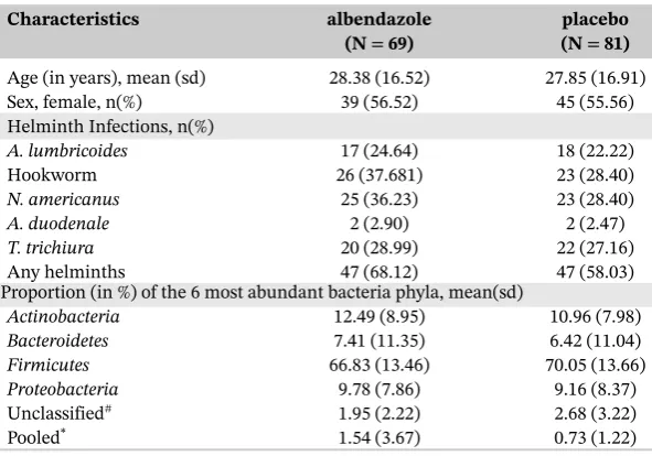
The baseline characteristics of the study participants were given in Table 4. In each of the randomization arms, there are four possible combinations of infection status at pre- and post-treatment, namely, uninfected subjects who either remained uninfected (condition 1) at post-treatment or became infected at post-treatment (condition 2) and infected subjects who either became uninfected at post-treatment (condition 3) or remained infected at post-treatment (condition 4). The number of samples in each conditions at pre- and post-treatment are given in Figure 4. It has been shown previously that treatment had an effect on the composition at post-treatment in infected subjects who remained

infected (condition 4).5 _{Here, we want to reanalyze this data set by using a joint model for the microbiome data at}

pre- and post-treatment to assess the treatment effect in the infected subjects who remained infected. Additionally, we want to estimate the time effect while adjusting for other variables such as infection status and treatment

alloca-tion. The following loglinear model is considered. LetD,E,F,G,H represent the categorical variables: bacterial taxa,

TABLE 4 Characteristics at baseline for study participants

Characteristics albendazole placebo

(N=69) (N=81)

Age (in years), mean (sd) 28.38 (16.52) 27.85 (16.91) Sex, female, n(%) 39 (56.52) 45 (55.56) Helminth Infections, n(%)

A. lumbricoides 17 (24.64) 18 (22.22)

Hookworm 26 (37.681) 23 (28.40)

N. americanus 25 (36.23) 23 (28.40)

A. duodenale 2 (2.90) 2 (2.47)

T. trichiura 20 (28.99) 22 (27.16)

Any helminths 47 (68.12) 47 (58.03)

Proportion (in %) of the 6 most abundant bacteria phyla, mean(sd)

Actinobacteria 12.49 (8.95) 10.96 (7.98)

Bacteroidetes 7.41 (11.35) 6.42 (11.04)

Firmicutes 66.83 (13.46) 70.05 (13.66)

Proteobacteria 9.78 (7.86) 9.16 (8.37)

Unclassified# _{1.95 (2.22) 2.68 (3.22)}

Pooled* _{1.54 (3.67) 0.73 (1.22)}

#_{Unclassified represents sequences that cannot be assigned to a phyla.}

*_{Pooled category consists of the remaining 13 phyla having average relative abundance among}

FIGURE 4 The profile of the microbiome study. The chart shows the number of subjecs infected with at least one of the prevalent soil transmitted helminths (Helminth (+)) or free of helminth infections (Helminth (-)) that belonged to either the placebo or albendazole treatment group, at pre-treatment and 21 months after the first treatment round. The circled number represents the condition explained in Section 4 [Colour figure can be viewed at wileyonlinelibrary.com]

infection (INF), treatment (TRT), baseline infection status (BHelm), and time (t) withJ,K,L,M,Nlevels for each

vari-able. For bacterial phyla, theFirmicuteswas considered as a reference category. Now, the following model was fitted to

the data

log (

𝜇DEFGH i𝑗klm

)

=(log(𝛿−1 0

)

+𝜆D_𝑗)+

(

𝜆E k +𝜆

DE

𝑗k

)

+(𝜆Hn +𝜆DH_𝑗n

)

+

(

𝜆FH ln +𝜆

DFH

𝑗ln

)

+(𝜆GHmn+𝜆DGH_𝑗mn

)

+

(

𝜆FGH lmn +𝜆

DFGH

𝑗lmn

)

+

(

𝜆EFGH klmn +𝜆

DEFGH

𝑗klmn

)

+ui

with the baseline constraint atJ=K=L=M=N=1, ui∼N

( 0, 𝜎2u

)

. (14)

Alternatively, the model could be written in terms of regression coefficients as follows:

log (

𝜇(t)

i𝑗

)

=𝜉0𝑗+𝜉1𝑗INF+𝜉2𝑗t+𝜉3𝑗TRT×t+𝜉4𝑗BHelm×t+𝜉5𝑗BHelm×TRT×t

+𝜉6_𝑗INF×BHelm×TRT×t+ui,

where𝜉0_𝑗 =log(𝛿−1

0 ) +𝜆D𝑗,𝜉1𝑗 =𝜆Fl +𝜆 DF

𝑗l , and so forth. In this model, there are 6 ×7 estimable covariate effects on each

bacterial phyla. In condition 4, the difference in the microbiome composition between the albendazole and placebo arm

is represented by𝜉3j+𝜉5j+𝜉6j, whereas, in condition 3, the difference in the microbiome composition between two arms

by𝜉3_j +𝜉5j. In the subjects who are uninfected at baseline, the treatment effect is represented by𝜉3j, irrespective of their

infection status at post-treatment. The change of microbiome composition, when subjects were uninfected at baseline,

remained uninfected at post-treatment, and received placebo, is modeled by𝜉2_j. Two interaction terms with BHelm were

included in this model (14) (ie, the coefficient𝜉4jand𝜉5j) to model the effect of having infection at pre-treatment and still

being infected at follow up, irrespective of treatment by albendazole. The coefficient𝜉4_jrepresents the effect of having

infection at pre-treatment in the placebo group. We first included a subject-specific random effectuiin the model.

Statisti-cal significance for each covariate was assessed by the likelihood ratio test with 6 degrees of freedom and the significance

of the random effect was assessed using the likelihood ratio test with mixture of𝜒2

[0,1]distribution.

The parameter estimates from the loglinear model with subject-specific random effects (14) are given in Table S8. The

between subject variation over time is estimated by the standard deviation𝜎uof 0.269 (s.e. of 0.053). The variance of this

random effect is significantly different from zero (p-value<0.001, LRT with mixture of𝜒2

[0,1]distribution), indicating that

the microbiome counts of a person over time are correlated. The regression coefficients for the covariates BHelm×t(𝜉4j)

and BHelm×TRT×t(𝜉5_j) appear not to be significantly associated with the microbiome (p−values>0.05), indicating that

having infection at pre-treatment does not influence the microbiome composition. These two covariates were present at

the second time point for subjects in conditions 3 and 4. Being the terms𝜉4_j+𝜉_5jalmost zero for all categories, the change

TABLE 5 The log odds ratio (95% CI) when data set were fitted with Dirichlet-multinomial mixed with categorical-specific random effect having common variance*

Categories INF t TRT×t Bhelm×INF×TRT×t

Actinobacteria −0.006 (−0.218, 0.207) 0.050 (−0.155, 0.256) 0.046 (−0.235, 0.326) 0.326 (−0.042, 0.694)

Bacteroidetes 0.220 (−0.056, 0.496) −0.119 (−0.395, 0.157) −0.012 (−0.381, 0.356) −0.916 (−1.573,−0.259)

Protobacteria 0.171 (−0.054, 0.396) 0.056 (−0.161, 0.273) 0.035 (−0.256, 0.326) 0.026 (−0.376, 0.427) Unclassified −0.024 (−0.304, 0.257) 0.129 (−0.149, 0.407) −0.099 (−0.476, 0.277) −0.159 (−0.727, 0.410) Pooled 0.166 (−0.158, 0.490) 0.195 (−0.124, 0.515) −0.030 (−0.449, 0.388) −0.180 (−0814, 0.454)

Loglik −8285.5 ̂𝜃(s.e) 0.08 (0.01)

̂𝜎u(s.e) 0.22 (0.03)

*_{Fitted with SAS procedure NLMIXED with 3 quadrature points of adaptive Gauss-Hermite approximation.}

To obtain a model with less parameters, we first eliminated the covariate BHelm×TRT×t. The covariate BHelm×twas

also not significant in this reduced model (p−value of 0.795). Hence, we reduced model (14) further by eliminating this

covariate. In this updated model, BHelm×TRT×twas still not significant (p−value of 0.843). Finally, we fitted the following

model:

log (

𝜇(t)

i𝑗

)

=𝜉0_𝑗+𝜉1_𝑗INF+𝜉2_𝑗t+𝜉3_𝑗TRT×t+𝜉4_𝑗INF×BHelm×TRT×t+ui. (15)

In this final model for fixed effects, assuming a subject-specific random effect (15), 6 × 4 parameters represent the

covariate effects on the microbiome composition. The treatment effect is modeled by𝜉3_j for all conditions except for

condition 4. The difference in the microbiome composition in condition 4 between the albendazole and placebo arm

is represented by𝜉_3j + 𝜉4_j. The estimated log odds ratio for each bacterial category compared toFirmicutesis given in

Table S9. Moreover, for this model, the standard deviation of random subject-specific effectuiis significantly greater than

zero (p−value<0.001). Albendazole has no direct effect in subjects who remained uninfected as the odds ratios for each

bacterial category are approximately 1. On the other hand, when subjects remained infected, the odds ofActinobacteria

toFirmicutesat the second time point compared to the first time point increases about 55%, whereas the odds ratio for BacteroidetestoFirmicutesdecreases about 62%.

Next, we considered a six-dimensional random effects structure for this data. We fitted DMM model (15). The results are listed in Tables 5 and S10. Overall, the estimates of the fixed effects and overdispersion are very similar for these random effect structures. This is in line with the result of the simulation study. However, when we fitted the DMM model with categorical-specific random effects, we observed the following. As the estimated variance component over time for the first

three categories are relatively large (𝜎2

u1=0.369 to𝜎

2

u3=0.536), for the last three categories (Proteobacteria, Unclassified

and Pooled) are small, and hence, the random effects for these categories can be omitted.

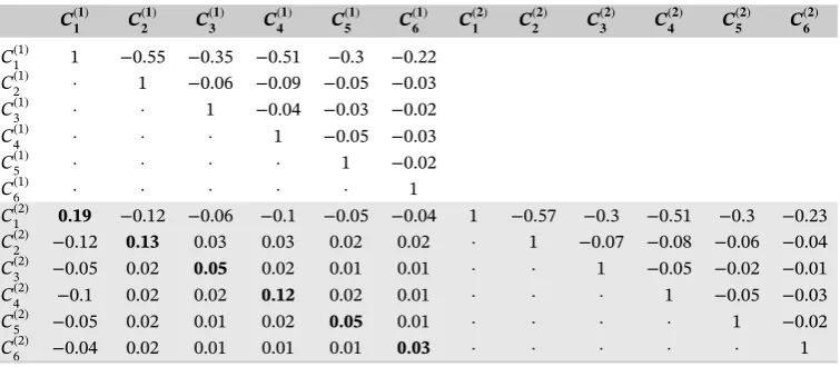
Finally, we investigated whether the correlations induced by the model correspond to the observed correlations; the marginal correlation induced by the DMM model with a subject-specific random effect (Table S11A), a categorical spe-cific random effect with common variance (Table 6) and with categorical-dependent variance for the random effects

TABLE 6 The estimated marginal correlation of the data set obtained by Dirichlet-multinomial mixed model with categorical-specific random effect having common variance across categories

C(_𝟏𝟏) C(_𝟐𝟏) C(_𝟑𝟏) C(_𝟒𝟏) C(_𝟓𝟏) C(_𝟔𝟏) C(_𝟏𝟐) C(_𝟐𝟐) C(_𝟑𝟐) C(_𝟒𝟐) C(_𝟓𝟐) C(_𝟔𝟐)

C₁(1) 1 −0.55 −0.35 −0.51 −0.3 −0.22

C₂(1) · 1 −0.06 −0.09 −0.05 −0.03

C₃(1) · · 1 −0.04 −0.03 −0.02

C₄(1) · · · 1 −0.05 −0.03

C₅(1) · · · · 1 −0.02

C₆(1) · · · 1

C₁(2) 0.19 −0.12 −0.06 −0.1 −0.05 −0.04 1 −0.57 −0.3 −0.51 −0.3 −0.23

C₂(2) −0.12 0.13 0.03 0.03 0.02 0.02 · 1 −0.07 −0.08 −0.06 −0.04

C₃(2) −0.05 0.02 0.05 0.02 0.01 0.01 · · 1 −0.05 −0.02 −0.01

C₄(2) −0.1 0.02 0.02 0.12 0.02 0.01 · · · 1 −0.05 −0.03

C₅(2) −0.05 0.02 0.01 0.02 0.05 0.01 · · · · 1 −0.02