Sensitivity of p-mode absorption on magnetic region properties and kernel functions

This is a repository copy of

Sensitivity of p-mode absorption on magnetic region properties

and kernel functions

.

White Rose Research Online URL for this paper:

http://eprints.whiterose.ac.uk/42883/

Article:

Gascoyne, A., Jain, R. and Hindman, B.W. (2011) Sensitivity of p-mode absorption on

magnetic region properties and kernel functions. Astronomy & Astrophysics, 526. Art no.

A93. ISSN 0004-6361

https://doi.org/10.1051/0004-6361/201015898

[email protected] https://eprints.whiterose.ac.uk/ Reuse

Unless indicated otherwise, fulltext items are protected by copyright with all rights reserved. The copyright exception in section 29 of the Copyright, Designs and Patents Act 1988 allows the making of a single copy solely for the purpose of non-commercial research or private study within the limits of fair dealing. The publisher or other rights-holder may allow further reproduction and re-use of this version - refer to the White Rose Research Online record for this item. Where records identify the publisher as the copyright holder, users can verify any specific terms of use on the publisher’s website.

Takedown

If you consider content in White Rose Research Online to be in breach of UK law, please notify us by

December 7, 2010

Sensitivity of p-Mode Absorption on Magnetic Region Properties

and Kernel Functions

Andrew Gascoyne

, Rekha Jain

and Bradley W. Hindman

1 Applied Mathematics Department, The University of Sheffi_{eld, S3 7RH (UK); app07adg@she}ffi_{eld.ac.uk, R.Jain@she}ffi_eld.ac.uk.

2 JILA, University of Colorado at Boulder (USA); [email protected]

Preprint online version: December 7, 2010

ABSTRACT

Aims.Magnetohydrodynamic (MHD) sausage tube waves are excited in magnetic flux tubes by p-mode forcing. These tube waves carry energy away from the p-mode cavity which results in a source of absorption. We wish to see the eff_{ect of an ensemble of}

ran-domly distributed thin magnetic flux tubes on the absorption of p-modes for the model plage region and also study the eff_{ect of the}

spacial weighting function on the theoretically calculated absorption coeffi_cients.

Methods.We calculate the absorption coeffi_{cients of p modes for a model plage, assumed to consist of an ensemble of many thin}

magnetic flux tubes with randomly distributed plasma properties. Each magnetic flux tube in the ensemble is modelled as axisymmet-ric, non-interacting, vertically oriented and untwisted.

Results.We find that the magnitude and the form of the absorption coeffi_{cient is sensitive to the plasma-βof the tubes which is}

con-sistent with previous work. Both the random distribution used to model the ensemble of flux tubes and the spatial weighting function inherent to the measurement of the absorption aff_{ect the absorption. As the width of the weighting function increases, the absorption}

increases.

Key words.Sun: helioseismology – Sun: oscillations – Magnetic fields – Magnetohydrodynamics (MHD) – Scattering

1. Introduction

Solar acoustic modes (p modes) are absorbed and scattered by magnetic inhomogeneities such as sunspots or plage regions. Scattering by such structures has been studied, using various observational helioseismic techniques (see Braun et al. 1988, Couvidat et al. 2006). Braun & Birch (2008) found that sunspots can absorb over half of incident p-mode power and plage regions can absorb around 20%. The measured “bell-shaped” tion has a well-established frequency dependence; the absorp-tion rises from zero at zero frequency, plateaus around 4 mHz and then suff_{ers a precipitous drop at higher frequencies; this}

drop off_{has now been deemed unphysical due to local emission}

at higher frequencies (Braun & Birch 2008).

This “bell-shaped” absorption had been known for decades (e.g., Braun et al. 1988) and theoretical models have been con-structed to interpret the frequency variation in an attempt to un-derstand the sub-structure of these magnetic regions. One pro-posed mechanism is mode conversion. Classical MHD wave theory reveals that where fast and slow magnetoacoustic waves share the same phase velocity (i.e., at the equipartition layer), transformation of acoustic wave energy occurs between these two waves (see, for example Crouch & Cally 2003). Other mech-anisms include resonant absorption (Hollweg 1988), mode mix-ing (D’Silva 1994) and excitation of tube waves through p-mode buff_{eting (Bogdan et al. 1996, Hindman & Jain 2008).}

Spruit (1981) derived the governing equations for two basic modes of oscillation for a thin magnetic flux tube: kink modes, which describe transverse, incompressive motions of the tube supported by magnetic tension, and sausage modes, which are longitudinal, compressive motions driven by the external pres-sure perturbations at the boundary between the tube and the non-magnetic medium. The excitation of tube waves through p-mode

buff_{eting was first introduced in Spruit (1991) and further}

ex-amined in Bogdan et al. (1996). Bogdan et al. (1996) calculated p-mode damping rates for such a mechanism using a photo-spheric stress-free boundary condition thus only allowing energy to be lost down the tube as the waves are reflected at the sur-face. To combat this issue of what surface boundary condition to use, Hindman & Jain (2008) introduced a maximal-flux con-dition whereby no reflection takes place at the surface, allowing energy to propagate above the surface. This boundary condition therefore, gives the other extreme of the stress-free condition, i.e., it places an upper limit on the energy lost to the solar atmo-sphere. Jain et al. (2009) studied this mechanism to calculate the absorption of p modes in a simulated plage region, comparing with observational results from Braun & Birch (2008).

In this paper we wish to study two diff_{erent e}ff_{ects: how}

do details of the observational kernel function which repre-sents the spatially weighted average of the magnetic flux around a point, modify the measured absorption coeffi_{cient and how}

2 Gascoyne et al: Sensitivity of p-Mode Absorption

2. Equilibrium Configuration

We consider magnetic fibril fields as axisymmetric magnetic flux tubes embedded in a plane-parallel, gravitationally stratified at-mosphere. We wish to study the excitation of magnetohydrody-namic (MHD) tube waves through the buff_{eting of the tubes by}

external acoustic oscillations residing beneath the solar photo-sphere.

2.1. Background Atmosphere

We model the nonmagnetic medium as a polytropic atmosphere with constant gravity acting downwards g=_{−gˆz; z is increasing}

upwards. The pressure, density and sound speed vary as power laws as follows:

Pext(z)=

gz0ρ0 a+₁ −

z z0

!a+1

=_{P0 −}z

z0 !a+1

, (1)

ρext(z)=ρ0 − z z0

!a

, (2)

c2_ext(z)=₋gz

a, (3)

where the subscript ’0’ refers to the value at the model photo-sphere. Following Bogdan et al. (1996), Hindman & Jain (2008) and Jain et al. (2009) we set the truncation depth at z = _−z0

which is the model photosphere where the quantitiesρ0and P0 are the values of the mass density and gas pressure at this depth. Above the truncation depth z>₋z0we assume the existence of a hot vacuum (ρext→0 with temperature Text→ ∞). The

exter-nal pressure, density and sound speed increase with depth and as our atmosphere is in convective equilibrium, the polytropic in-dex a is related to the ratio of specific heatsγvia a=_1/(γ−1).

We also set the following characteristic physical scales for our model photosphere,ρ0 =2.78×10−7g cm−3, P0 =1.21×105 g cm−1 s−1, and g =_2.775×104 _{cm s}−1_{, which coincide with}

the photospheric reference model of Maltby et al. (1986). The choice of polytropic index a = _{1.5 yields the truncation depth}

z0=392 km and a photospheric sound speed of 8.52 km s−1.

2.2. Slender Magnetic Tube Configuration

We assume the magnetic field is comprised of thin magnetic flux tubes with the following properties:

– Vertically aligned with the z-axis. – Untwisted and axisymmetric.

– Embedded inside the field-free polytropic atmosphere. – Potential magnetic field, thus force free (i.e., no internal

cur-rents).

– Thin such that the tube’s radius is much smaller than any characteristic length scale such as the atmospheric scale lengths and the wavelength of tube waves.

– Flux tube interior has the same temperature variation with depth as the surrounding polytrope.

For such a thin magnetic flux tube to be in hydrostatic and ther-modynamic balance requires that temperature and total pressure are uniform across the tube and equal to the external values. Thus the magnetic pressure has the same scale height as the gas pres-sure, which results in a constant plasma-βwith height within the tube. Since the gas pressure decreases rapidly with height in the solar atmosphere so does the magnetic pressure; this then results

in significant flaring of field lines which inevitably breaks the thin flux tube approximation. This is the reason for truncating the polytrope at a depth which ensures that the thin flux tube ap-proximation is valid. The radial variation of the magnetic field is ignored (see Bogdan et al. 1996 for details). Thus the tube’s in-ternal pressure P(z), densityρ(z), magnetic field B(z), and cross-sectional area A(z) can be described as follows,

P(z)= β

β+₁Pext(z), (4)

ρ(z)= β

β+₁ρext(z), (5)

B2(z) 8π =

1

β+₁Pext(z), (6)

A(z)= θ

B(z)=

β+₁

8πPext(z) !1/2

θ. (7)

It is important here to point out the relationship between A(z), B(z) andθfor a single tube. For any given flux tube we are free to specify only two of the four parameters: the photospheric radius R0 (or cross-sectional area A0 =πR2₀), the magnetic fluxθ, the photospheric field strength B0and the plasma-β. Once specified, these two are the two remaining parameters are determined by equations (6) and (7).

The next step is to simulate a plage region by considering a random distribution of flux tubes. We choose to restrict our attention to a range ofβvalues between 0 and 2, spanning the strong to weak field regimes. We shall use three diff_erent

ran-dom distributions, a uniform distribution so all βvalues have equal probability, thus meanβ=_{1. We shall also consider a}

nor-mal (Gaussian) distribution of flux tubes with meanβ= _{1 and}

variance 1 (or e-folding length of 1). The final distribution we shall take is an exponential distribution such that the probability decreases asβincreases with meanβ=_{0.2 and variance 1. For}

simplicity we shall assume that every individual tube has equal magnetic fluxθ. This means that changingβhas the eff_{ect of}

changing the radius of the tube (see equation (7)).

3. Wavefield description

The field-free atmosphere supports resonant acoustic oscilla-tions (f and p modes) that are trapped in a waveguide below the model photosphere. The upper boundary of the waveguide is the photosphere itself while the lower boundary is refractive, arising from the linear increase in temperature with depth.

3.1. Wave equations

In the field-free atmosphere, for wave perturbations p′

ext, ρ′ext,

ξ′, in pressure, density and fluid displacement, respectively, we have the following linearized hydrodynamic equations,

ρ′_ext+_ξ′

k ∂ρext

∂z +ρext(∇·ξ

′₎=_{0, (8)}

p′_ext+_ξ′

k ∂Pext

∂z

+_{γPext(∇·ξ}′₎=_{0, (9)}

ρext

∂2_ξ′ ∂t2 +∇p

′

whereξ′

k =ξ′·ˆz. By eliminating p′extandρ′extand substituting

ξ′ = _∇Φ_whereΦ_{is the displacement potential we obtain the}

following partial diff_{erential equation,}

∂2_Φ ∂t2 =c

2

∇2Φ_−g∂Φ

∂z. (11)

Here we have dropped the subscript on c2ext because, as

men-tioned earlier, the temperature variation inside and outside the tube is the same.

The incident acoustic wavefield expressed by equation (11) supports plane wave solutions of the form,

Φ_(x,t)=_Aei(kx−ωt)_{Q(z), (12)}

where_A is the complex wave amplitude,ω the temporal fre-quency, and k the horizontal wavenumber. Q(z) is the vertical eigenfunction. Substituting equation (12) into (11) generates the following ordinary diff_{erential equation}

"

c2 d 2

dz2 −g d dz+(ω

2 −k2c2)

#

Q(z)=_{0. (13)}

3.2. Boundary Conditions

Using the physical boundary conditions that the solution van-ishes deep in the atmosphere and the Lagrangian pressure per-turbations vanishes at the surface (i.e., at the truncation depth z=_{−z0), the solutions to equation (13) form a set of orthogonal}

eigenfunctions,

Q(z)=_w−(µ+1/2)_{Wκ, µ(w), (14)}

which depends on the following dimensionless parameters,

w=_{−2kz, µ}=(a−1)

2 , ν

2₌aω2z0

g , κ

= ν

2

2kz0.

Vanishing Lagrangian pressure perturbation at the up-per boundary (∇ · ξ′ = _{0), at z} = _{−z0, requires the}

following quantization condition (see Bogdan et al. (1996) or Hindman & Jain (2008) for details),

Wκ, µ+1 ν2

κ !

=_{0. (15)}

The eigenvaluesκhave a discrete set of values. For the spe-cial case of a “complete” polytrope, where z0=0, the eigenval-ues take the special formκn =1/2+µ+n. In our more general

case, with z0,0, theκnmust be generated numerically from the

roots of equation (15).

4. Absorption via the Excitation of Tube Waves

Here we consider the absorption of acoustic waves arising from the excitation of magnetic tube waves. We ignore the excitation of the acoustic jacket and the existence of mode mixing (see Bogdan & Cally 1995 for a full investigation into the presence of laterally evanescent jacket modes and Gordovskyy et al. 2009 for an explanation of the role of mode mixing in p-mode absorp-tion).

4.1. Magnetic Flux Tube Oscillations

We are seeking waves on thin tubes that lack internal struc-ture. Only three types of MHD waves satisfy this criterion: tor-sional Alfv´en waves, longitudinal (sausage) waves and trans-verse (kink) waves. We ignore torsional Alfv´en waves because the p-mode oscillations are irrotational when the atmosphere is adiabatically stratified and therefore do not couple with torsional waves. In this paper we will also ignore the kink waves and specifically concentrate on axisymmetric oscillations. Using the formulation of Jain et al. (2009), the fluid displacement due to the excitation of sausage waves within the tube can be described by the following equation,

∂2 ∂t2 +

2gz 2a+_β(1+_a)

∂2 ∂z2 +

g(1+_a)

2a+_β(1+_a)

∂ ∂z

! ξ_k

=(1+a)(β+1)

2a+_β(1+_a)

∂3_Φ

∂z∂t2. (16)

These sausage wavesξ_k(z,t) can be described as axisymmet-ric pressure pulses that produce displacements that are primarily parallel to the magnetic field. The p-mode driving term appears on the right hand side of equation (16) through the displacement potential Φ_{. This equation can be put in nondimensional form}

as,

d2 ds2 +

µ+₁

s d ds +ν 2_ǫ s ! ξ_k =A

z0

f (s), (17)

where,

s=₋z

z0

, ǫ= 2a+β(1+a)

2a , f (s)=−

(1+_a)(β+₁₎

2a ν2

s dQ(s)

ds .

The homogeneous version of equation (17) has the following solution,

ψ_k(s)=_s−µ/2_Hµ(1)_(2ν√_{ǫs), (18)}

where H is the Hankel function (Abramowitz & Stegun 1964) andψ_k(s) represents a downward propagating sausage wave and its complex conjugateψ∗

k(s) represents the upward propagating wave.

4.2. Absorption Coefficient for a Single Tube

In order to calculate the absorption of a single thin magnetic flux tube, we follow the calculation presented in Jain et al. (2009) and Hindman & Jain (2008). Quoting their result for the absorp-tion coeffi_{cient α due to the generation of sausage waves, we}

have

α= πβ

2(2+_γβ)(β+₁₎

λa+1 ν2_H

A0 z2 0

(_|Ω +_I∗_|2+_|I|2_{− |}Ω_|2+_{S), (19)}

S=₋(1+a)(β+1)

2a ν

2_Q 0

H_µ(1)2ν√ǫ(Ω +_I∗₎

+_H(2) µ

2ν√ǫ(Ω∗+_I)

, (20)

whereλ=ν2_/κand

H is an integral associated with the lateral energy flux carried by any individual wave component (see Jain et al. 2009, eqn. (11)). The integral

I= Z ∞

1

4 Gascoyne et al: Sensitivity of p-Mode Absorption

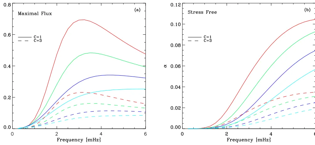
Fig. 1. Absorption coeffi_{cient calculated as a function of frequency for a simulated plage consisting of a number of flux tubes for two di}ff_erent

BC. Each tube is assumed to be of the sameβ(=_{1). Each panel shows the absorption coe}ffi_{cient for two di}ff_{erent kernel function. One has much}

broader wings (_C=_{1) than the other (C}=_{3). Each mode order is represented by a di}ff_{erent colour: red (p1), green (p2), blue (p3) etc.}

describes the interaction between the p mode and the sausage wave.

The parameterΩ _{in equation (19) represents the boundary}

condition (BC) at the surface s = _{1 (or z} = _{−z0). Similar}

to Jain et al. (2009) we take two separate BC at the surface, a stress-free and a maximal-flux condition. As mentioned in _§1, the stress-free BC has the physical interpretation that all upward propagating waves are reflected at the surface. Maximal-flux BC can be interpreted as no wave reflection at the surface, thus all upward propagating waves escape into the upper atmosphere. For a detailed explanation of how to calculateΩ_{for these two}

BC see Hindman & Jain (2008); here we simply quote their re-sult,

Ω_{S F}=_i(1

+_a)(β+₁₎

aπ ν

2Q0 R −

R∗

RI, (22)

for stress-free BC where,

R=_ν√_ǫH(1) µ+1

2ν√ǫ+_(β+_1)(µ+_1)H(1) µ

2ν√ǫ,

and,

Ω_MF=₋(1+a)(β+1)

2a ν

2_Q 0Hµ(2)

2ν√ǫ, (23)

for maximal-flux BC.

4.3. Absorption for a Random Ensemble of Tubes

We wish to apply our theory to model the absorption coeffi_cient

measured for a typical solar plage region by examining the eff_ect

of a large number of thin magnetic flux tubes. We thus assume that the tubes are suffi_{ciently separated so as to neglect the e}ff_ect

of multiple scattering.

In order to compute the number of tubes N required to esti-mate the collective absorption coeffi_{cient of a plage we follow}

Jain et al. (2009). We use a spatial weighting function or ker-nel K, which linearly relates the distribution of magnetic flux in

the plage region, to the observed absorption. LetΘ_{(r, ω) be the}

amount of magnetic flux sampled by an observation,

Θ_{(r, ω)}= Z

K(r′₋r, ω)_|B(r′)_|dr′, (24)

where K(r, ω) is the kernel, and as Jain et al. (2009) assumed,

K(r, ω)=_e−k2|r|2/π2_{, (25)}

where k (=_ω2 a

2κg) is the horizontal wavenumber. N, the number

of flux tubes, is equal to the magnetic flux sampled by the kernel function Θ_{divided by the magnetic flux of an individual flux}

tubeθ,

N=Θ(r, ω)

θ . (26)

It is thus clear that N is dependent on the form of the spatial weighting function. We shall investigate the eff_{ect of various}

ker-nel functions by including a constant_Cin the spatial weighting function K as follows,

K(r, ω)=_e−Ck2|r|2/π2_{. (27)}

Increasing the value of_Cnarrows the width of the kernel func-tion K(r, ω) and decreases the magnetic fluxΘ_{(r, ω) (see eqn.}

24), thereby reducing the number of tubes required (vice versa for decreasing_C).

To calculate the total absorptionαtotfor the various

distribu-tions of tubes as discussed earlier in_§2.2 we generate a random collection of N tubes, each with a diff_{erent value of βi drawn}

from the desired probability distribution. The collective absorp-tion is then,

αtot = N X

i=1

α(βi), (28)

whereα(βi) is the absorption for a single tube and the sum is

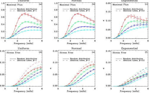
Fig. 2. Mean absorption coeffi_{cient with error bars calculated as a function of frequency for a simulated plage, for various random distributions in}

β. Over-plotted with dashed lines is the case for simulated plage with identical tubes ofβequal to the meanβof the distribution. Each mode order is denoted by a diff_{erent colour: red (p1), green (p2), blue (p3), etc.}

5. Results and Discussion

In this section we present the results for theoretically calculated absorption coeffi_{cients of p modes by the generation of magnetic}

tube waves in the convection zone through external p-mode buf-feting. In particular, we investigate the eff_{ect of a distribution of}

flux tube plasma-β. We considerθto be the same for every tube in this model.

5.1. Effect of Kernel function on the Absorption Coefficient

It was previously noted in Jain et al. (2009) that a poor approx-imation for the observation kernel will give a poor approxima-tion for the number of flux tubes necessary to simulate the plage region. Here we wish to explicitly examine the eff_{ect of various}

constants_Cin the Gaussian kernel function on the absorption co-effi_{cientsα. In figure 1 we plot absorption coe}ffi_{cients forC}=₁

and 3 for the two separate boundary conditions. Increasing the value of this constant_C, narrows the kernel, resulting in a smaller value for the parameter N (see equations (26) and (27)). This clearly reduces the amount of p-mode absorption for the sim-ulated plage. Here we have assumed that each flux tube in the plage is identical with the sameβ(=_{1) value.}

Clearly the absorption coeffi_{cient is sensitive to the width of}

the kernel function. Knowing accurate kernel functions used for observationally measuredαin magnetic regions is thus crucial in correctly interpreting the amount of absorption observed.

5.2. Effect of a Random Collection of Flux Tubes on Absorption Coefficients

Jain et al. (2009) assumed that each flux tube in the simulated plage had the same value ofβ. However, intuitively, this is un-likely to be the case for real solar plage regions. Thus, here we consider magnetic fibrils with a random distribution ofβvalues, ranging from 0 to 2 as discussed in_§4.3. We use three diff_erent

random distributions, uniform, normal (Gaussian), and an expo-nential distribution and plot our results in figure 2. We gener-ated 40 separate realisations for a given distribution then plotted the mean absorption coeffi_{cient for this ensemble of realisations}

(solid curve). The error bars represent the standard deviation ofα within these 40 realisations. For comparison we have also over-plotted, with dashed lines, the case of a simulated plage where each flux tube is now assumed to have sameβ, i.e., a collection of identical tubes withβequalling the meanβof the comparison distribution.

For maximal-flux BC, the solid and dashed curves are in good agreement with each other, whereas the stress-free BC shows larger deviations. This is due to the fact that the absorption coeffi_{cient is almost linear withβ(forβ <2) for maximal-flux}

BC, whereas for the stress-free BC, it is nonlinear (this is ex-plicitly explored in Jain et al. 2010). This eff_{ect is more for low}

radial orders since these waves are confined closer to the surface where the dynamics are more dominated by the upper boundary condition.

or-6 Gascoyne et al: Sensitivity of p-Mode Absorption

der. This behaviour is due to the parameter N (the number of tubes required), which, because of its dependence on the ker-nel, decreases as the horizontal wavenumber increases. The hori-zontal wavenumber increases with frequency and decreases with mode order. For high value for the number N we have a larger sample size and thus lower errors, and vice versa for low N.

For the two upper BC used here, the maximal-flux condition produces the most promising results at a first glance when com-paring with observations (see Braun and Birch 2008). The stress-free condition lacks the fall off_{as seen in the observed}

absorp-tion coeffi_{cients at higher frequencies. However the unphysical}

nature of this fall off_{(see Braun and Birch 2008) suggests that}

extra caution should be taken when interpreting the observations. Also, in reality the actual reflection at the solar photosphere is likely to lie in between these two extreme conditions.

6. Conclusions

In this paper we have presented a calculation for the absorption coeffi_{cient for a collection of vertical, axisymmetric, thin}

mag-netic flux tubes designed to simulate a solar plage region. The absorption mechanism used here is the generation of longitu-dinal (sausage) tube waves through buff_{eting of the magnetic}

fibrils by external solar p modes. The generation of these tube waves carry energy out of the p-mode cavity and thus result in the absorption of p modes.

We infer that there are a number of factors to consider when investigating the absorption of p modes by magnetic regions. In particular, the eff_{ect of the upper boundary condition, the}

obser-vational kernel used to estimate the “eff_{ective” number of tubes}

in a plage and the distribution of plasma-βamongst the collec-tion of flux tubes. Besides local emission at high frequencies, other factors such as the amount of reflection from the surface, the plasma properties of the flux tubes in an ensemble and the form of the spacial weighting function all have considerable ef-fect on the absorption coeffi_cient.

The small size of the error bars (see figure 2) tells us that given the observed absorption coeffi_{cient for an active region,}

we can be confident on the likely distribution ofβthat best fits this observed active region. Thus if one can obtain a good match between theory and observations we have a good diagnostic tool with which to measure the statistical properties of the flux tubes within a plage.

Acknowledgements. This work is supported by UK STFC studentship.

References

Abramowitz, M., & Stegun, I. A. 1964, Handbook of Mathematical Functions (New York: Dover)

Bogdan, T. J., & Cally, P. S. 1995, ApJ, 453, 919

Bogdan, T. J., Hindman, B. W., Cally, P. S., Charbonneau, P. 1996, ApJ, 465, 406

Braun, D. C., Duvall, T. L., & LaBonte, B. J. 1988, ApJ, 335, 1015 Braun, D. C., & Birch, A. C. 2008, Solphys., 251, 267

Cally, P. S., Crouch, A. D., & Braun, D. C. 2003, MNRAS, 346, 381 Couvidat, S., Birch, A. C., & Kosovichev, A. G. 2006, ApJ, 640, 516 Crouch, A. D., & Cally, P. S. 2003, Sol. Phys., 214, 2011

D’Silva, S. 1994, ApJ., 435, 881

Gordovskyy, M., Jain, R., Hindman, B. W. 2009, ApJ, 694, 1602 Hanasoge, S. M., & Cally, P. S. 2009, ApJ., 697, 651

Hindman, B. W., & Jain, R. 2008, ApJ, 677, 769 Hollweg, J. V. 1988, ApJ, 335, 1005

Jain, R., Hindman, B. W., Braun, D. C., & Birch, A. C. 2009, ApJ, 695, 325 Jain, R., Gascoyne A., Hindman, B. W. 2010, MNRAS, Submitted.

Maltby, P., Avrett, E. H., Carlsson, M., Kjelsdeth-Moe, O., Kurucz, R. L., & Loeser, R. 1986, ApJ, 306, 284

Spruit, H. C. 1981, A&A, 98, 155