This is a repository copy of
An empirical study of hyperheuristics for managing very large
sets of low level heuristics
.
White Rose Research Online URL for this paper:
http://eprints.whiterose.ac.uk/75049/
Version: Submitted Version
Article:
Remde, Stephen, Cowling, Peter I. orcid.org/0000-0003-1310-6683, Dahal, Keshav P. et
al. (2 more authors) (2012) An empirical study of hyperheuristics for managing very large
sets of low level heuristics. Journal of the Operational Research Society. pp. 392-405.
ISSN 1476-9360
https://doi.org/10.1057/jors.2011.48
[email protected] https://eprints.whiterose.ac.uk/ Reuse
Items deposited in White Rose Research Online are protected by copyright, with all rights reserved unless indicated otherwise. They may be downloaded and/or printed for private study, or other acts as permitted by national copyright laws. The publisher or other rights holders may allow further reproduction and re-use of the full text version. This is indicated by the licence information on the White Rose Research Online record for the item.
Takedown
If you consider content in White Rose Research Online to be in breach of UK law, please notify us by
An Empirical Study of Hyperheuristics for Managing Very Large Sets of
Low Level Heuristics
Stephen Remde1, Peter Cowling1, Keshav Dahal1, Nic Colledge1, Evgeny Selensky2
1
Artificial Intelligence Research Centre, University of Bradford, Bradford, BD7 1DP, United Kingdom
2
Trimble MRM Ltd. (EMEA), 1 Bath Street, IP City Centre, Ipswich, IP2 8SD, United Kingdom
{s.m.remde, p.i.cowling, k.p.dahal, n.j.colledge}@bradford.ac.uk, [email protected]
Abstract. Hyperheuristics give us the appealing possibility of abstracting the solution method from the problem, since our
hyperheuristic, at each decision point, chooses between different low level heuristics rather than different solutions as is
usually the case for metaheuristics. By assembling low level heuristics from parameterised components we may create
hundreds or thousands of low level heuristics, and there is increasing evidence that this is effective in dealing with every
eventuality that may arise when solving different combinatorial optimisation problem instances since at each iteration the
solution landscape is amenable to at least one of the low level heuristics. However, the large number of low level heuristics
means that the hyperheuristic has to intelligently select the correct low level heuristic to use, to make best use of available
CPU time. This paper empirically investigates several hyperheuristics designed for large collections of low level heuristics
and adapts other hyperheuristics from the literature to cope with these large sets of low level heuristics on a difficult
real-world workforce scheduling problem. In the process we empirically investigate a wide range of approaches for setting tabu
tenure in hyperheuristic methods, for a complex real-world problem. The results show that the hyperheuristic methods
described provide a good way to trade off CPU time and solution quality.
Keywords: Computational Analysis, Heuristics, Hyperheuristics, Machine Learning, Optimization, Scheduling, Tabu
Search
1 Introduction
heuristic(s) to apply at each decision point. The hyperheuristic method does not need to be problem specific, and hence a single hyperheuristic method has the advantage that it can work generally across many problem models and instances, given the right set of low level heuristics and solution quality metrics. There is good evidence to date that hyperheuristics are effective across a range of problems, and this effectiveness arguably arises since having a large collection of low level heuristics means that the solution landscape for one or more of these low level heuristics is likely to provide a good search direction (Chakhlevitch and Cowling, 2005) (Colledge, 2009) (Remde et al, 2009).
In some cases low level heuristics are parameterised, or composed by “multiplying” together components (Remde et al, 2007) (Chakhlevitch and Cowling, 2005), which can give rise to hundreds or even thousands of heuristics (Cowling and Chakhlevitch, 2003). In such a case, deciding in reasonable time which heuristics to use may be difficult. However, there is evidence that having such a rich selection of low level heuristics may yield better results for complex problems in the long run, although it is difficult to know in advance which low level heuristics will prove effective (Chakhlevitch and Cowling, 2005). (Remde et al, 2007) studied the low level heuristics used by a greedy hyperheuristic HyperGreedy (which picks the best performing low level heuristic at each iteration) and found that a quarter of the low level heuristics were never used and half of the low level heuristics were effective less than one percent of the time. However, the low level heuristics which were effective varied from problem instance to problem instance, and it was difficult to predict which low level heuristics would prove effective. In this paper we investigate hyperheuristic approaches that attempt to learn which low level heuristics will perform poorly and ignore them to produce solutions of a quality similar to those produced using the full set of low level heuristics, in a fraction of the CPU time. This is particularly of interest since hyperheuristic methods have demonstrated their effectiveness at solving problems such as automated planograms (Bai and Kendall, 2005), examination scheduling (Burke et al, 2003), personnel scheduling (Cowling et al, 2003), workforce scheduling (Remde et al, 2007) and artificial intelligence in computer games (Nareyek, 2004). These applications have shown that hyperheuristics offer some of the solution quality we would associate with tailored methods, but that they are very flexible in dealing with different problem instances (and indeed different problems) and that they remain effective when the problem is changed in significant ways, without requiring substantial intervention from a human expert (Kendall and Hussin, 2005a).
and Chao, 1999) and Vehicle Routing Problem with Time Windows (VRPTW) (Toth and Vigo 2001). In this real-world situation we have several further constraints and objectives, and in particular we consider the notion of the degree of competence of a particular group of resources (e.g. engineers) which have been allocated to a particular task. Trimble MRM Ltd. develops scheduling solutions for very large, complex mobile workforce scheduling problems in a variety of industries, particularly telecommunications and utilities. The model which we investigate here encapsulates the main features common to these problems.
We use the problem and the hyperheuristic framework of (Remde et al, 2007) as a test bed for our investigation in this paper. The complexity of this problem means that quality evaluation of a perturbed solution takes a significant amount of CPU time, whereas limited amounts of CPU time are available to find good solutions in practice. Many of the low level heuristics in our hyperheuristic framework require the evaluation of hundreds of these perturbed solutions, due to them solving smaller parts of the problem optimally using systematic search or investigating a large neighbourhood. The available CPU time renders local search based hyperheuristics infeasible in our practical application, so that we will only consider constructive hyperheuristics in this paper. The number of low level heuristics available to the hyperheuristics is large compared to the number of those low level heuristics we will apply in constructing a solution, and new approaches are needed to learn the effectiveness of low level heuristics in this case. (Chakhlevitch and Cowling, 2005) find that when selecting a small random subset of low level heuristics results can be erratic across different problem instances indicating that a reduced subset is not as good as a large set.
This paper is structured as follows: we present related work in Section 2. Our problem is presented in section 3. Section 4 describes the hyperheuristic framework and hyperheuristics in detail. In section 5 we empirically investigate the techniques and compare them to Variable Neighbourhood Search, Greedy, Random and Tabu search based heuristics in terms of solution quality and computational time. We present conclusions in Section 6.
2 Related Work
Many hyperheuristics are based on metaheuristic methods, including early work in (Fang, 1994) where a genetic algorithm evolved a chromosome which determined how jobs were scheduled in open shop scheduling. In (Bai and Kendall, 2005) simulated annealing is used to decide whether to accept the solution resulting from a randomly applied low level heuristic. (Kendall et al, 2002) uses a Genetic Algorithm to evolve good sequences of low level heuristics. (Chakhlevitch and Cowling, 2005) use a learning approach called Step-by-Step Reduction (SSR) and Warming Up (WU) to reduce the number of low level heuristics and show that SSR produced better results. SSR removes a percentage of the low level heuristics periodically to try and reduce the set to an elite few. This removes bad heuristics early on and saves CPU time that would have been used trying them, but suffers from the potential limitation that it does not allow the reintroduction of these heuristics later in the search. The work of (Remde et al, 2007) shows that a low level heuristic’s effectiveness is highly variable during search with some low level heuristics which are ineffective at the start of search proving highly effective at the end.
Tabu Search (Glover and Laguna, 1997) is used to stop the repeated application of poor moves or the undoing of good moves for a certain number of iterations (the tabu tenure). The optimal duration of tabu tenure has been tested in several papers and it is most likely a function of the neighbourhood size and the problem size (Laguna
et al, 1999). Using random tabu tenures, where a move is made tabu for a period chosen uniformly at randomly
tenures are utilised. Random tabu tenures provide results of similar quality to those with fixed tenure equal to the expected random tenure on the two examination timetabling problem instances they consider. They find that repeated application of a low level heuristic does not increase solution quality considerably, possibly due to an increased tendency to get stuck in large basins of attraction. A large set (95) of low level heuristics is used in (Cowling and Chakhlevitch, 2003) where the hyperheuristic allows a tabu low level heuristic to become
aspirated and be used (Glover and Laguna, 1997) if it makes the best improvement. If no improving low level
heuristic is available, a non-improving non-tabu low level heuristic is used and made tabu. Fixed tabu tenures of 10, 30, 60 and 100 and adaptive tabu tenures are investigated, but results provide no clear advantage of using adaptive tabu tenures over fixed ones. A ranking system, based on reinforcement learning, is used for non-tabu low level heuristics in (Burke et al, 2003). At each iteration the non-tabu low level heuristic with the highest rank is applied. When a non-tabu low level heuristic performs well its rank is increased, otherwise its rank is decreased and the low level heuristic is put in the tabu list on a first in first out basis. If the highest ranked low level heuristic makes the solution worse, the tabu list is emptied.
Nareyek (Nareyek, 2004) experimentally investigates several variations of reinforcement learning in a hyperheuristic framework. Different reinforcement schemes are used in two different problems and it is concluded that high rates of negative reinforcement and low rates of positive reinforcement work best. The choice function (Cowling et al, 2001) is another machine learning hyperheuristic that attempts to estimate how well a low level heuristic is likely to perform based on its effect on the (single) objective function, the pair-wise interaction between low level heuristics and the time since it was last used. These two papers combine ideas from machine learning and tabu search.
The hyperheuristic framework of (Remde et al, 2007) proposes a method to break down the Trimble MRM workforce scheduling problem, by splitting it into smaller parts and solving each part using exact enumerative approaches. These smaller parts are the combination of a method to select a task and a method to select potential resources, including time, for the task. Reduced Variable Neighbourhood Search (rVNS) (Mladenovic and Hansen, 1997) and simple hyperheuristics are shown to be effective in deciding the order in which to solve sub-problems.
3 Problem Description
The workforce scheduling problem that we consider consists of four main components: Tasks, Resources, Skills and Locations. A taskTi is a job or part of a job. Each task must start and end at a specified location. Usually the start and end locations are the same, but they may be different. Each task has one or more time windows and some time windows have an associated penalty. We have a set {T1,T2,…,Tn} of tasks to be completed. Each task is executed by one or more resources {R1,R2,…,Rm}. A task requires resources with the appropriate skills from the set {S1,S2,…,Sk}. Task Ti requires skills [TS1i,TS2i,...,TSti(i)] with work requirements
[
w
1i,
w
2i,...,
w
it(i)]
wherei q
w
is the amount of skillTS
qi required for task Ti. Task Ti also has an associated priority p(Ti). Resource Rj possesses skills [RS1j,RS2j,...,RSrj(j)]. A function c(R,S) expresses the competence of resource R at skill S,relative to an average competency. Each resource R travels from location to location at speedv(R). For tasks T1,
T2, d(T1, T2) is the distance between the end location of T1 and the start location of T2.
There are three main groups of constraints: task constraints, resource constraints and location constraints:
Task constraints
Each task can be worked on only within specified time windows.
Some tasks require other tasks to have been completed before they can begin (precedence constraints).
Some tasks require other tasks to be started at the same time (assist constraints).
Tasks may be split across breaks within a working day.
For a task to be scheduled it must have exactly one resource assigned to it for each of the skills it requires.
All assigned resources have to be available at the task’s location for its whole duration regardless of their skill competency and task skill work requirement.
If a task Ti with skill requirements [TS1i,TS2i,...,TSti(i)] and amounts
[
1,
2,...,
()]
i i t i i
w
w
w
is carried out by resources [R1, 2,..., i()]i t i
i R R then the time taken is
(1)
(i.e. the greatest time taken for any single resource to complete a skill requirement).
Resource constraints
A resource R travels from location to location at a fixed speed v(R).
{1max,2,...,()} ( , i) q i q i q i t
q c R TS
Resources may only work and travel during specified time windows.
Resources can only work on one task at a time and only apply one skill at a time.
Location constraints
Resources (generally engineers in vans or large pieces of equipment) must travel to the start location of each task they work on, and are unavailable during this travel time.
Resources must start and end each day at a specified “home” location and must have sufficient time to travel to and from their home location at the start and end of each day.
When building a schedule many different and often contradictory business objectives are possible. In this paper we consider three objectives. The first objective is Schedule Priority (SP), given by
(2)
Maximising Schedule Priority maximises the value of the tasks scheduled and implicitly minimises the value of tasks unscheduled.
The second objective measures total Travel Time (TT) across all resources. Define A={(i1,i2,j):task Ti1comes immediately before Ti2in the schedule of resource Rj}.
(3)
Travel to and from home locations is handled by considering dummy tasks fixed at the start and end of the working day, at the home location of each resource.
The third objective measures the inconvenience associated with completing tasks or using resources at an inconvenient time, which we have labelled Schedule Cost (SC). In order to express this accurately we express the time windows for Resource R using a function X (Baptiste et al, 2001) where X(R,t) is the cost per unit time for resource R working at time t. We introduce a variable
otherwise 0 at time ng) or traveli task a (on busy is resource if 1 ) ,
(Rt R t
Similarly we introduce X’ where X’(T,t) is the cost per unit time for task T being executed at time t and
otherwise 0 at time executed being is task if 1 ) , (
'Tt T t
(4)
In this paper, the fitness of a schedule is given by a single weighted objective function, f = SP - 4SC - 2TT, where SP is the sum of the priority of scheduled tasks, SC is the sum of the resource and task time window costs in the schedule and TT is the total amount of travel time. This objective is to maximise the total priority of tasks scheduled while minimising travel time and cost. Values are scaled so that this expression is a realistic representation of solution quality for a large class of problems encountered in practice (Cowling et al, 2006).
4 Hyperheuristic Approaches
Previous hyperheuristic work on this workforce scheduling problem (Remde et al, 2007), (Remde et al, 2009) generated possible low level heuristics (LLHs) by combining two components: (1) selecting the next task to be scheduled and (2) allocating potential resources (including time) for that task. The task selector (table 1) chooses a task and the resource allocator (table 2) assigns resources for each skill required by the task, so that the total number of low level heuristics is the number of task selectors multiplied by the number of resource allocators (fig. 1 shows how the low level heuristics work). Note that where a resource allocator is parameterised, we consider each parameter set as an individual resource allocation heuristic. We combine each of the 9 different task selectors with each of the 27 different resource allocators to give a total of 243 low level heuristics. Our low level heuristics maintain a feasible solution – if the low level heuristic cannot make a legal move then the solution is not modified.
The hyperheuristic HyperRandom (Remde et al, 2007), selects at random a low level heuristic (i.e. a (task order, resource allocator) pair) to use at each iteration and applies it if the application will result in an improvement. This continues until no improvement has been found for a certain number of iterations.
HyperGreedy (Remde et al, 2007) evaluates all the low level heuristics at each iteration and applies the best if it
makes an improvement. This continues until no improvement is found. As might be expected, HyperGreedy is very CPU-intensive, but generates good quality results.
As the low level heuristics are constructive, we can only apply each one a small number of times before the schedule is full, since approximately 250 tasks can fit in the schedule of the problems we study, compared to 243 low level heuristics. Hyperheuristics which rely on learning from the application of a low level heuristic during a single long search run would be ineffective, as the schedule would be full before significant
m j t j j n i t ii t T t dt R t R t dt
information has been learnt. Note that it is coincidental that the number of low level heuristics and the number of tasks is similar in this case. Reinforcement learning based hyperheuristics need to be modified in this case to learn from all different low level heuristics tried in a situation and not simply the one that was applied in the end, otherwise the vast majority of information gained about low level heuristics would be discarded. This paper investigates and empirically compares hyperheuristic performance in this situation.
Section 4.1, 4.2 and 4.3 describes the hyperheuristics which attempt to learn information about the low level heuristics and their potential to improve the solution.
4.1 Binary Exponential Back Off
Binary Exponential Back Off (BEBO) is a tabu search based hyperheuristic with dynamically adapting tabu tenures designed for very large neighbourhoods, inspired by the binary exponential back-off algorithm used as the industry standard to transmit packets in a network (Kwak et. at., 2005). It aims to increase network throughput by exponentially increasing the time between retransmits when a collision occurs. This happens when two or more computers try to transmit information on the same medium (a wire, a wireless frequency, etc) at the same time. When a collision occurs, the device will increase its backoff value by 1, and wait a random amount of time between 0 and 2backoff-1 before trying to retransmit. If the transmission is successful, the back off value is reset to 0, otherwise the back-off value is increased by 1 again and the process is repeated. Hence waiting time increases exponentially for low level heuristics in this case.
We use an analogous backing off method to exponentially increase the tabu tenure of low level heuristics which repeatedly yield no improvements, meaning the expected time between trials of bad heuristics increases exponentially. Pseudocode for the hyperheuristic is given in fig. 2. We use two methods to decide which of the low level heuristics, that were tried in the current iteration, to back off (those “deemed bad”): BEBO Best x: only the best x improving low level heuristics are not backed off, and, BEBO Prop x: all non-improving low level heuristics and those improving low level heuristics not in the top x% of the range of the fitness are backed off.
backoff_min is set to 4 as it provided good results in (Remde et al, 2009). Although no empirical investigation
4.2 Reinforcement Learning
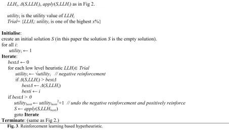
Reinforcement learning is a machine learning technique that positively reinforces good choices and negatively reinforce bad choices (Kaelbling et al, 1996). Nareyek (Nareyek, 2004) proposes a reinforcement learning hyperheuristic framework to investigate several approaches to learning empirically. A utility value is associated with each choice which estimates its future potential. At each iteration a choice is made based on these utility values and then the utility value is adjusted depending on the outcome of that choice and the learning mechanism used. Five methods for positively reinforcing the utility and five methods for negatively reinforcing the utility are experimentally evaluated, and in general low rates of positive reinforcement and high rates of negative reinforcement gave best results. In our experiments, we will use the adaptation scheme which was found to be best in (Nareyek, 2004). For positive reinforcement ui:=ui+1 and ui:=√ui for negative reinforcement of low level heuristic i.
Nareyek’s experiments ran for ten thousand iterations and the number of low level heuristics was very small (5 and 6 in the two different problems). This means that each heuristic could be applied many times giving the hyperheuristic time to learn. In the problem we study this ratio is drastically reduced and since our low level heuristics (choices) nearly always make a positive change in terms of fitness, this means that modification of the hyperheuristic will be needed.
At each iteration, a number of the low level heuristics with the highest utility will be tried instead of just one. The best performing of the selected low level heuristics will be positively reinforced and applied and the rest negatively reinforced. The percentage we try will give us the ability to trade off CPU time and solution quality. The pseudocode for the reinforcement learning hyperheuristic is given in fig. 3. In our computational experiments, the heuristic Nareyek x% signifies low level heuristics whose utility is in the top x% will be tried.
4.3 Tabu Search Based Hyperheuristics
We try tabu tenures of t=5, 7, 10, 25, 50 each time a low level heuristic is tried and fails to give an improvement. We also investigate different methods of deciding which LLHs to make tabu. Tabu Best x t=y
signifies that all but the top x improving low level heuristics will be made tabu with tenure y at each iteration. This is similar to the method used in (Burke et al, 2003), with larger tabu tenures since there are more low level heuristics in our case. We also investigated making all non-improving low level heuristics tabu however the results for these were very poor in terms of CPU time as nearly all of the low level heuristics make a positive improvement early in the search although this improvement is very small. These results are not reported here. In addition to these fixed tenures, we try random tenures as used in (Kendall and Hussin, 2005a): rTabu Best x t=y is similar to Tabu Best x t=y, but with a random tenure between 0 and y each time a low level heuristic is made tabu.
4.4 Other Methods
We compare these adapted methods to existing ones designed for large neighbourhoods and problem specific heuristics.
rVNS is the best reduced Variable Neighbourhood Search method taken from (Remde et al, 2007) and is a
hand crafted tailored heuristic for this problem. HyperRandom and HyperGreedy are the random and greedy hyperheuristics from (Remde et al, 2009). HyperGreedy will be the benchmark for all the tests as this is the most CPU-intensive approach and generally produces the best result. Sample x% is variation of HyperRandom.
In this Hyperheuristic, x% of the low level heuristics are sampled uniformly at random and the best improving one is applied.
Step-by-Step reduction is presented in (Chakhlevitch and Cowling, 2005). The method SSR x% t=y reduces the set of low level heuristics by x% every y iterations. The ones which have performed the worst over the period, as measured by the objective value, are removed first, ties are broken randomly.
5 Computational Experiments
and three skills and resources possess between one and five skills. The problems reflect realistic problems Trimble have identified and are generated using a commercial problem instance generator (Cowling et al, 2006). The size of the problems was chosen to be solvable in a reasonable amount of CPU time. Over 218 CPU days was needed to complete the all experiments for the problem instances, so the experiments were run in parallel on 88 cores of 22 identical 4 core 2.0 GHz machines. Implementation was done using C# .NET under Microsoft Windows Vista.
We compare the average performance in terms of CPU time and solution quality of the 62 methods based on 9 different hyperheuristic approaches with different parameters (rVNS, HyperGreedy, HyperRandom, 9 BEBO
“Best x”, 7 BEBO “Prop x”, 15 “standard” Tabu, 7 Nareyek based, 16 Step-by-Step Reduction and 7 Random
Sampling hyperheuristics). Table 3 summarises each of these categories of heuristics. The experimental results,
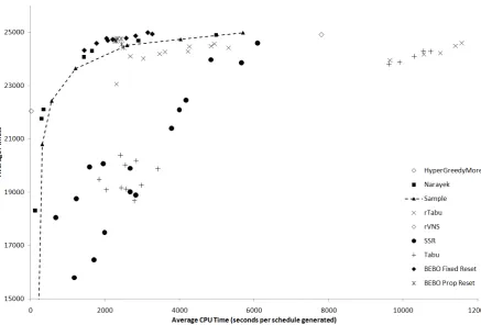
average fitness and CPU time along with its parameter for each of these hyperheuritics, are presented in table 4. Note that only the best results in terms of CPU time and fitness are shown for BEBO, rTabu and Tabu due to the limited space. The complete results for these three approaches are given in reference (Remde et al, 2009). Fig. 5 depicts some selected results for comparing the hyperheuristics performances. The table and graph show the results of the different solution methods with various parameters. The line connecting the points in fig. 5 is for
the Sample heuristic which is a naïve approach to trading off CPU time and solution quality. Hyperheuristics
which are making better-than-random choices of low level heuristics are above the line connecting the Sample
points in fig. 5. For the Sample hyperheuristic, we can see that it can effectively use additional CPU time to generate higher quality solutions, and indeed that it provides a continuum of improving results with increased CPU time. Sample 80% produces better results than HyperGreedy in less CPU time, probably due to its avoiding consistently applying the same low level heuristics at each iteration, providing a useful and effective source of diversification.
wasteful of this CPU time compared to other approaches. Sample 80% generates better solutions on average in slightly less CPU time, the BEBO Best 20 hyperheuristic generates better results in less than half the CPU time
of HyperGreedy. Other hyperheuristics approach the solution quality of HyperGreedy in a fraction of the CPU
time, notably BEBO Prop 0.01%, rTabu Best 10 t = 7, Nareyek 80% and SSR 5% t = 20, suggesting that all these approaches contain interesting ingredients. Still HyperGreedy remains a good benchmark against which to judge other approaches.
Step-by-Step Reduction (SSR) performs poorly in comparison to the other hyperheuristics. (Remde et al, 2007) provides evidence that some low level heuristics only begin to work well towards the end of a search and it is likely that SSR is discarding these due to low performance at the start of the search and then failing to find a good solution because these low level heuristics are needed toward the end of the search. It is notable that SSR
approaches appear to have a near-linear improvement following a poor start, and that SSR approaches which discard only a small number of low level heuristics per iteration perform well, for modest CPU time savings compared to HyperGreedy.
The fixed tabu tenure hyperheuristics (Tabu) perform poorly in comparison to the random tabu tenure hyperheuristics (rTabu), supporting the conclusions of (Rolland et al, 1996) (Kendall and Hussin, 2005a). The Tabu results are all well below the threshold given by the Sample points, indicating that these approaches perform significantly worse than random choice per second of CPU time. The rTabu results are only slightly below the Sample threshold line, and they do give modest improvements with increasing CPU time, but are not competitive with Sample, Nareyek and BEBO approaches.
The performance of Nareyek approaches is consistently better than that of the Sample approach with respect to CPU time and fitness. Nareyek approaches are capable of beating Sample using similar, small amounts of CPU time. The reinforcement learning technique used is shown to be effective, and certainly better than a random approach, in selecting good low level heuristics. The CPU times of the Sample and Nareyek
hyperheuristics that consider a similar number of low level heuristics (Sample 1% and Nareyek 1%, Sample 10%
and Nareyek 10% etc) are quite different due to the fact that some of the better low level heuristics take more
CPU time and the Nareyek hyperheuristic identifies these and uses them more frequently than Sample. Hence
Nareyek approaches offer some control of CPU time and are the best among those studied at low-to-moderate
CPU times.
implementation of BEBO cannot produce results in smaller amounts of CPU time. Increasing min_backoff could make this hyperheuristic faster, although our experiments show a decline in solution quality in this case. BEBO
Prop is slightly less effective than BEBO Best for slightly more CPU time, which agrees with the conclusions of
(Remde et al, 2009).
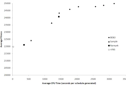
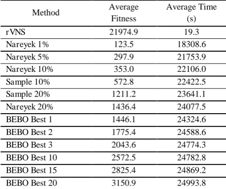
Table 5 and fig. 6 show the Pareto frontier of these results which contains the heuristics giving optimal trade-offs between CPU time and solution quality. As mentioned earlier, the dominance of the tailored rVNS heuristic for small CPU time is apparent, then for low to moderate CPU time Nareyek and Sample dominate. The appearance of the random Sample approach in the Pareto frontier is unexpected, but an inspection of fig. 5 shows that there are few approaches consuming CPU time in this range. The absence of a Nareyek
hyperheuristic in this range is due to the difficulty of tuning the Nareyek parameters to obtain a precise CPU time when the hyperheuristic is choosing between low level heuristics which take very different amounts of CPU time. This difficulty of tuning the CPU time applies also to BEBO and Tabu approaches. BEBO dominates the other methods when more CPU time is available, indeed the BEBO Best 20 approach dominates approaches which consume more than twice as much CPU time (which are shown in fig. 5 but not in fig. 6).
confidence. Overall, it appears that BEBO, Sample and Nareyek methods outperform SSR and Tabu
hyperheuristics in terms of fitness alone, and even more so if we also consider CPU time.
6 Conclusions
This paper investigates and compares several hyperheuristic approaches which handle a large number of low level heuristics, on a difficult real-world scheduling problem. Our low level heuristics are generated by combining parameterised components for (i) choosing which task to schedule; and (ii) allocating resources to the chosen task, giving us a large set of over 200 low level heuristics. Since a large number of low level heuristics are available, our intuition suggests that at each step the solution landscape is amenable to at least one of the low level heuristics. Our results, in comparison to a tailored reduced Variable Neighbourhood Search approach, and an approach which greedily searches through all low level heuristics at each step, suggest that this is an effective way to produce high quality solutions, albeit in large amounts of CPU time.
The problem we consider contains features common to many real-world scheduling problems which deal with mobile resource management (occurring in pick up/delivery, project management, routing and maintenance applications). The approach to generating low level heuristics can generalise across these problems, so that our hyperheuristic approaches and results give an indication of the effectiveness of these techniques for a wide range of complex mobile workforce scheduling problems.
When using a large collection of low level heuristics, we must decide between different low level heuristics at each iteration rather than choosing directly between different solutions. Several methods are presented for choosing between low level heuristics, which are generally applicable since they make use only of fitness information. A thorough empirical investigation is undertaken to determine the effectiveness of these techniques in using increasing amounts of CPU time to effectively generate high quality solutions.
heuristics which have high utility. This method performs well when low to medium CPU time is available, and surpasses the random sampling method. The Binary Exponential Back Off method increases the tabu tenure for a poorly performing heuristic exponentially, and resets the penalty to a small value for low level heuristics which perform well. This approach is dominant for medium to high amounts of CPU time and again beats a random sampling approach on average for a given CPU time.
A Step by Step Reduction method, which discards poorly performing low level heuristics during search, does not perform well in this case where the number of iterations to generate a solution is small, since it appears to discard early on low level heuristics which are important later in the search. While this approach works reasonably well when the number of heuristics discarded is small and CPU time is high, it is outperformed by a random sampling technique when the number of low level heuristics discarded is high.
When analysing the Pareto frontier representing the best trade off between fitness and CPU time, the Nareyek-based approaches dominate for smaller CPU times, and the Binary Exponential Back Off Nareyek-based approaches dominate for large amounts of CPU time. “Gaps” in the CPU time used, which arise due to difficulty in
precisely controlling the total amount of CPU time of a hyperheuristic when choosing between low level heuristics which consume variable amounts of CPU time, are taken by random sampling approaches, in preference to step-by-step reduction and tabu search approaches.
Overall, the methods described in this paper show that hyperheuristics provide an effective way to trade off CPU time for solution fitness, when solving complex real-world scheduling problems, and provide empirical comparisons between a wide range of hyperheuristic approaches (62 parameter sets of 9 different hyperheuristic approaches). It will be interesting, in further work, to extend the range of hyperheuristics investigated to approaches which are effective when the user stops the search and the amount of CPU time is not known in advance.
References
Bai R and Kendall G (2005). An Investigation of Automated Planograms using a Simulated Annealing Based
Hyperheuristics. In: Ibaraki T, Nonobe K, and Yagiura M (eds). Meta-heuristics: Progress as Real Problem Solvers,
Selected Papers from the 5th Metaheuristics International Conference (MIC 2003), Springer, 87-108.
Baptiste P, Le Pape C and Nuijten W (2001). Constraint Based Scheduling. Kluwer Academic Publishers: London.
Burke E, Kendall G and Soubeiga E (2003). A Tabu-search Hyperheuristic for Timetabling and Rostering. Journal of
Burke E, Hyde M, Kendall G, Ochoa G, Özcan E and Woodward J (2010). A Classification of Hyperheuristic Approaches.
In: Gendreau M and Potvin J-Y (eds). Handbook of Metaheuristics, Springer, 449-468.
Chakhlevitch K and Cowling P (2005). Choosing the Fittest Subset of Low Level Heuristics in a Hyperheuristic Framework.
In: Raidl G, Gottlieb J (eds). Proc. of Evolutionary Computation in Combinatorial Optimization. Springer LNCS 3448,
23-33.
Chakhlevitch K and Cowling P (2008). Hyperheuristics: Recent Developments. In: Cotta C, Sevaux M and Sorensen K
(eds). Adaptive and Multilevel Metaheuristics, Studies in Computational Intelligence vol 136, Springer, 3-29.
Colledge N (2009). Evolutionary Approaches to Dynamic Mobile Workforce Scheduling. PhD Thesis. University of
Bradford, UK.
Cowling P, Kendall G and Soubeiga E (2001). A Hyperheuristic Approach to Scheduling a Sales Summit, In: Proc. of
selected papers from the 3rd International Conference on the Practice and Theory of Automated Timetabling (PATAT
2000), Springer LNCS 2079, 176-190.
Cowling P and Chakhlevitch K (2003). Hyperheuristic for Managing a Large Collection of Low Level Heuristics to
Schedule Personnel. In: Proc. of the 2003 IEEE Congress on Evolutionary Computation (CEC2003). IEEE Press,
1214-1221.
Cowling P, Colledge N, Dahal K and Remde S (2006). The Trade Off between Diversity and Quality for Multi-objective
Workforce Scheduling. In: Jens G, Günther R (eds). Proc. of Evolutionary Computation in Combinatorial
Optimization, Springer LNCS 3906, 13-24.
Fang H, Ross P and Corne D (1994). A Promising Hybrid GA/Heuristic Approach for Open-Shop Scheduling Problems. In
Hölldobler S, Lutz C, Wansing H (eds). Proc. of the 11th European Conference on Artificial Intelligence, 590-594.
Glover F and Laguna M (1997). Tabu Search. Springer.
Kaelbling L, Littman M and Moore A (1996). Reinforcement Learning: A Survey. Journal of Artificial Intelligence Research
4: 237–285.
Kendall G, Han L, and Cowling P (2002). An Investigation of a Hyperheuristic Genetic Algorithm Applied to a Trainer
Scheduling Problem. In: Fogel D, El-Sharkawi M, Yao X, Greenwood G, Iba H, Marrow P and Shackleton M (eds).
Proc. of Congress on Evolutionary Computation 2002, IEEE Press, 1185-1190.
Kendall, G and Hussin, N (2005a). A Tabu Search Hyperheuristic Approach to the Examination Timetabling Problem at the
MARA University of Technology. In: Burke E and Trick M (eds). Proc. of selected papers from the 5th International
Conference on the Practice and Theory of Automated Timetabling (PATAT 2004), Springer LNCS 3616, 270-293.
Kendall, G and Hussin, N (2005b). An Investigation of a Tabu Search Based Hyperheuristic for Examination Timetabling.
In: Kendall G, Burke E and Petrovic S (eds). Proc. of the Multidisciplinary Scheduling: Theory and Applications
Kolisch R and Hartmann S (2006): Experimental Investigations of Heuristics for RCPSP: An Update. European Journal of
Operational Research 174(1): 23-37.
Kwak B, Song N and Miller L (2005). Performance Analysis of Exponential Backoff, IEE-ACM Transactions on
Networking 13(2): 343-355.
Laguna M, Marti R and Campos V (1999). Intensification and Diversification with Elite Tabu Search Solutions for the
Linear Ordering Problem. Computers & Operations Research 26 (12): 1217-1230.
Mladenovic N and Hansen P (1997). Variable Neighborhood Search. Computers & Operations Research 24 (11): 1097-1100.
Miller R (1997). Beyond ANOVA: Basics of Applied Statistics. Texts in Statistical Science Series, Chapman Hall, London.
Nareyek A (2004). Choosing Search Heuristics by Non-stationary Reinforcement Learning. In: De Sousa J (eds). Applied
Optimization 86: 523-544.
Pinedo M and Chao X (1999). Operations Scheduling with Applications in Manufacturing and Services. McGraw-Hill, New
York.
Remde S (2009). Enhanching the Performance of Heuristic Search. PhD Thesis, University of Bradford, UK.
Remde S, Cowling P, Dahal K and Colledge N (2007). Exact/Heuristic Hybrids using rVNS and Hyperheuristics for
Workforce Scheduling. In: Cotta C, van Hemert J (eds). Proc. of Evolutionary Computation in Combinatorial
Optimization. LNCS 4464, 188-197.
Remde S, Cowling P, Dahal K, and Colledge N (2009). Binary Exponential Back Off for Tabu Tenure in Hyperheuristics.
In: Cotta C, Cowling P (eds). Proc. of Evolutionary Computation in Combinatorial Optimization. LNCS 5482,
109-120.
Rolland E, Schilling D and Current J (1996). An Efficient Tabu Search Procedure for the p-median Problem. European
Journal of Operational Research 96: 329–342.
Toth P and Vigo D (2001). The Vehicle Routing Problem. SIAM Monographs on Discrete Mathematics and Applications,
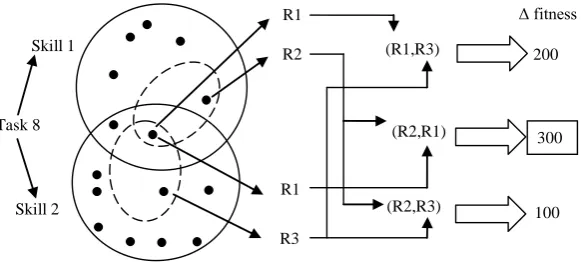
Fig 1. Resource allocators. The dotted subset of resources possessing the required skill is chosen by a Resource allocator. The assignment (R2, R1) is chosen as the best insertion.
Define:
LLHi is a low level heuristic i (whose application leads to a valid solution).
(S,LLHi) returns the change in the objective function resulting from applying low level heuristic LLHi to solution S.
apply(S,LLHi) returns the new solution we get after applying low level heuristic LLHi to solution S.
tabui is the Tabu tenure of LLHi (0≤ Tabui≤backoffi)
backoffi is the backoff value of LLHi (backoff_min≤ backoffi)
Eligible = {LLHi: tabui=0}
backoff_min is the minimum backoff value
Initialise:
create an initial solution S (in this paper the solution S is the empty solution). for all i:
backoffi backoff_min
choose tabui uniformly at random in {0,1,2,…, backoffi}
Iterate:
while(Eligible ≠{}) best 0
for each low level heuristic LLHi
Eligibleif (S,LLHi) > 0
backoffi backoff_min
if (S,LLHi) > best best (S,LLHi)
besti i
else
if LLHiis “deemed bad” (see text)
backoffi 2 * backoffi
choose tabui uniformly at random in {0,1,2,…, backoffi} for each low level heuristic LLHiEligible
tabui tabui –1
if best > 0 then
S apply(S,LLHbesti) go to Iterate Terminate:
for each low level heuristic LLHi
if (S,LLHi) > 0 S apply(S,LLHbesti)
go to Iterate
Fig. 2. The Binary Exponential Back Off (BEBO) hyperheuristic.
R1
R3 Skill 1
Skill 2
R1
R2 (R1,R3)
[image:20.595.152.443.72.203.2] [image:20.595.62.523.287.732.2]Define:
LLHi, (S,LLHi), apply(S,LLHi) as in Fig 2.
utilityi is the utility value of LLHi
Trial= {LLHi: utilityi is one of the highest x%}
Initialise:
create an initial solution S (in this paper the solution S is the empty solution). for all i:
utilityi 1
Iterate: best 0
for each low level heuristic LLHi
Trialutilityi √utilityi // negative reinforcement
if (S,LLHi) > best best (S,LLHi)
besti i
if best > 0
utilitybesti utilitybesti2+1 // undo the negative reinforcement and positively reinforce
S apply(S,LLHbesti) goto Iterate
Terminate: (same as Fig 2.)
Fig. 3. Reinforcement learning based hyperheuristic.
Define:
LLHi, (S,LLHi), apply(S,LLHi) as in Fig 2.
rank(i) is the rank of the (S,LLHi)in descending order.
tabui is the tabu tenure of LLHi
keep is the number of best performing low level heuristics that will not be made tabu.
Initialise:
create an initial solution S (in this paper the solution S is the empty solution). for all i:
tabui 0
Iterate: best 0
for each low level heuristic LLHisuch that tabui=0
if (S,LLHi) > best best (S,LLHi)
besti i
for each low level heuristic LLHisuch that tabui>0
tabui tabui –1
for each low level heuristic LLHisuch that(tabui=0 and (S,LLHi) 0 and rank(i) >keep) tabui tabu_tenure // or choose tabuirandomly from {1,2,…, tabu_tenure}
if best > 0
S apply(S,LLHbesti) goto Iterate
Terminate: (same as Fig 2.)
[image:21.595.75.522.77.697.2] [image:21.595.69.523.82.343.2]Fig. 5. Comparison of hyperheuristics which yield solutions having greater than 15000 fitness on average, with respect to
CPU time and average solution quality. Each plotted point represents a parameter setting of the corresponding
[image:22.595.80.518.93.389.2]Fig. 6. Pareto optimal set of hyperheuristics showing non-dominated solutions with respect to average CPU time and
[image:23.595.74.513.65.369.2]solution quality.
Table 1. Task selectors
Method Description
Random Tasks are ordered at random.
PriorityDesc Tasks are ordered by their priority in descending order
RealPriortiyDescending Tasks are ordered by their priority multiplied by the number of resources required in descending order
PriorityAsc Tasks are ordered by their priority in ascending order PrecedenceAsc Tasks are ordered by their number of precedences ascending PrecedenceDesc Tasks are ordered by their number of precedences descending
PriOverReq Tasks are ordered by their estimated priority per hour assuming the task will take as long as the total skill requirement
PriOverMaxReq Tasks are ordered by their estimated priority per hour assuming the task will take as long as the maximum skill requirement
[image:23.595.67.543.490.661.2]Table 2. Resource allocators. Each parameter set yields a separate resource allocation heuristic (e.g. Best 1-5; Deviation
25%).
Name Description
Best x-y Orders the available resources by their competency at the task then chooses the resources ranked from x to y in the list. (x-y values considered are: 1-5, 6-10, 11-15, 16-20, 21-25, 26-30, 31-35, 36-40, 1-10, 11-20, 21-30, 31-40, 1-2, 3-4, 5-6, … etc, 2-3, 3-4, 4-5, …etc, 1-4, 3-6, 5-8, 7-10, … etc, 5-14, 15-24, 25-34.
Deviation x Resources complete a skill in a time dependent upon their competence. This selector attempts to find resources that will complete the different skills of task in the same amount of time by selecting resources with competencies that deviate x{50%, 25%, 12.5%, 6.25%} from the task’s skill requirement.
xth Quarter This picks the x{1,2,3,4} quarter of task ranked by skill. Unlike the “Top x” task selectors, the number chosen is proportionate to the number of resources who can do the task.
xth Eighth This picks the x{1…8} eighth of task ranked by skill.
Dynamic x This selector picks larger sets of resources for the skills requiring more effort and less to those requiring less effort. It will create x{10, 50, 100, 1000} combinations when enumerating the resulting sets.
[image:24.595.66.527.115.314.2]All Resources Considers all possible resources (and hence is very slow).
Table 3. Summary of hyperheuristics.
Heuristic Description
rVNS The best of a selection of fast handcrafted reduced Variable Neighbourhood Search based
heuristic from a large experimental study (Remde et al, 2007).
HyperGreedy A Greedy Hyperheuristic that samples all low level heuristics at each iteration and applies the
best one.
BEBO Best A Binary Exponential Back-Off based hyperheuristic backing off all but a fixed number of the
best performing low level heuristics.
BEBO Prop A Binary Exponential Back-Off based hyperheuristic backing off all but the low level
heuristics performing within a percentage of the best performing low level heuristic.
Nareyek A Machine learning hyperheuristic based on (Nareyek, 2004) reinforcement learning
experiments which tries a fixed number of low level heuristics with the highest utility.
Sample A random hyperheuristic which tries a percentage of the low level heuristics at each iteration
and applies the best one.
SSR The Step-by-Step Reduction hyperheuristic of (Chakhlevitch and Cowling, 2005) which removes a percentage of the poorest performing low level heuristics every few iterations.
Tabu A Tabu search based hyperheuristic that selects the best non-tabu low level heuristic and
makes a number of non-tabu poor performing low level heuristic tabu for a fixed number of iterations.
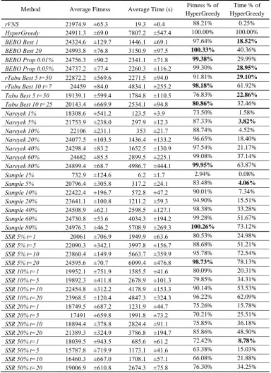
[image:24.595.65.524.374.632.2]Table 4. Average fitness and CPU time of each hyperheuristic and parameters. Only the best results for BEBO, rTabu, Tabu
in terms of CPU time and Fitness are shown. Full results for these hyperheuristics can be found in (Remde et al, 2009).
Results show 95% confidence intervals.
Method Average Fitness Average Time (s) Fitness % of
HyperGreedy
Time % of HyperGreedy
rVNS 21974.9 ±65.3 19.3 ±0.4 88.21% 0.25%
HyperGreedy 24911.3 ±69.0 7807.2 ±547.4 100.00% 100.00%
BEBO Best 1 24324.6 ±129.7 1446.1 ±69.1 97.64% 18.52% BEBO Best 20 24993.8 ±76.8 3150.9 ±97.5 100.33% 40.36%
BEBO Prop 0.01% 24756.3 ±90.2 2341.1 ±71.8 99.38% 29.99%
BEBO Prop 0.05% 24737.2 ±77.4 2260.3 ±116.2 99.30% 28.95% rTabu Best 5 t=50 22872.2 ±569.6 2271.5 ±94.0 91.81% 29.10% rTabu Best 10 t=7 24459 ±84.0 4834.1 ±255.2 98.18% 61.92%
Tabu Best 5 t=50 19139.1 ±599.4 1784.8 ±110.5 76.83% 22.86% Tabu Best 10 t=25 20143.4 ±669.9 2534.1 ±94.8 80.86% 32.46%
Nareyek 1% 18308.6 ±541.2 123.5 ±3.9 73.50% 1.58%
Nareyek 5% 21753.9 ±238.0 297.9 ±12.3 87.33% 3.82% Nareyek 10% 22106 ±231.1 353 ±21.7 88.74% 4.52% Nareyek 20% 24077.5 ±103.5 1436.4 ±133.2 96.65% 18.40%
Nareyek 40% 24298.4 ±83.2 1652.5 ±130.9 97.54% 21.17%
Nareyek 60% 24682 ±85.5 2899.5 ±225.1 99.08% 37.14%
Nareyek 80% 24899.4 ±68.7 4986.7 ±444.1 99.95% 63.87%
Sample 1% 732.9 ±124.6 6.2 ±1.7 2.94% 0.08%
Sample 5% 20796.4 ±305.8 317.2 ±24.1 83.48% 4.06% Sample 10% 22422.4 ±196.7 572.8 ±47.2 90.01% 7.34% Sample 20% 23641.1 ±100.8 1211.2 ±59.3 94.90% 15.51%
Sample 40% 24508.9 ±62.1 2598.5 ±127.1 98.38% 33.28%
Sample 60% 24730.8 ±53.6 4034.3 ±194.2 99.28% 51.67%
Sample 80% 24976.3 ±46.2 5708.9 ±269.3 100.26% 73.12%
SSR 5% t=1 20061 ±706.9 1949.9 ±63.6 80.53% 24.98%
SSR 5% t=5 22090.3 ±342.1 3997.8 ±156.7 88.68% 51.21%
SSR 5% t=10 23860.4 ±149.9 5663.7 ±359.9 95.78% 72.54%
SSR 5% t=20 24595.6 ±70.7 6099.4 ±476.8 98.73% 78.13%
SSR 10% t=1 19952.1 ±751.9 1585.5 ±41.6 80.09% 20.31%
SSR 10% t=5 19892.3 ±411.8 2678.9 ±101.3 79.85% 34.31%
SSR 10% t=10 22454.8 ±312.2 4178.9 ±153.3 90.14% 53.53%
SSR 10% t=20 23968.5 ±120.4 4847.3 ±324.3 96.22% 62.09% SSR 20% t=1 18749.5 ±687.2 1231.9 ±44.7 75.26% 15.78%
SSR 20% t=5 17491 ±659.8 1991.8 ±73.2 70.21% 25.51%
SSR 20% t=10 18894.4 ±378.8 2824.4 ±91.1 75.85% 36.18%
SSR 20% t=20 21389.3 ±324.9 3786.8 ±194.7 85.86% 48.50%
SSR 50% t=1 18039.5 ±943.5 685.6 ±61.2 72.42% 8.78% SSR 50% t=5 15787.8 ±719.9 1173.1 ±41.6 63.38% 15.03%
SSR 50% t=10 16460.3 ±667.0 1708.1 ±57.1 66.08% 21.88%
Table 5. Pareto optimal methods with respect to average fitness and CPU time.
Method Average
Fitness
Average Time (s)
rVNS 21974.9 19.3
Nareyek 1% 123.5 18308.6
Nareyek 5% 297.9 21753.9
Nareyek 10% 353.0 22106.0
Sample 10% 572.8 22422.5
Sample 20% 1211.2 23641.1
Nareyek 20% 1436.4 24077.5
BEBO Best 1 1446.1 24324.6
BEBO Best 2 1775.4 24588.6
BEBO Best 3 2043.6 24774.3
BEBO Best 10 2572.5 24782.8
BEBO Best 15 2825.4 24869.2
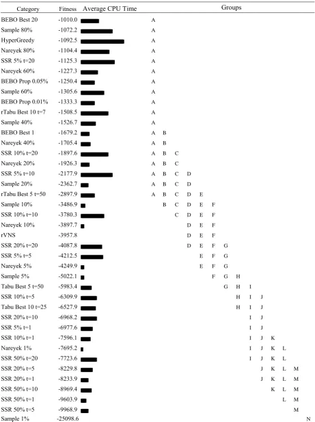
Table 6. Tukey analysis of hyperheuristic methods using a 95% confidence interval. CPU times are also shown.
Category Fitness Average CPU Time
Groups
BEBO Best 20 -1010.0 A
Sample 80% -1072.2 A
HyperGreedy -1092.5 A
Nareyek 80% -1104.4 A
SSR 5% t=20 -1125.3 A
Nareyek 60% -1227.3 A
BEBO Prop 0.05% -1250.4 A
Sample 60% -1305.6 A
BEBO Prop 0.01% -1333.3 A
rTabu Best 10 t=7 -1508.5 A
Sample 40% -1526.7 A
BEBO Best 1 -1679.2 A B
Nareyek 40% -1705.4 A B
SSR 10% t=20 -1897.6 A B C
Nareyek 20% -1926.3 A B C
SSR 5% t=10 -2177.9 A B C D
Sample 20% -2362.7 A B C D
rTabu Best 5 t=50 -2897.9 A B C D E
Sample 10% -3486.9 B C D E F
SSR 10% t=10 -3780.3 C D E F
Nareyek 10% -3897.7 D E F
rVNS -3957.8 D E F
SSR 20% t=20 -4087.8 D E F G
SSR 5% t=5 -4212.5 E F G
Nareyek 5% -4249.9 E F G
Sample 5% -5022.1 F G H
Tabu Best 5 t=50 -5983.4 G H I
SSR 10% t=5 -6309.9 H I J
Tabu Best 10 t=25 -6527.9 H I J
SSR 20% t=10 -6968.2 I J
SSR 5% t=1 -6977.6 I J
SSR 10% t=1 -7596.1 I J K
Nareyek 1% -7695.2 I J K L
SSR 50% t=20 -7723.6 I J K L
SSR 20% t=5 -8229.8 J K L M
SSR 20% t=1 -8233.9 J K L M
SSR 50% t=10 -8969.4 K L M
SSR 50% t=1 -9603.9 L M
SSR 50% t=5 -9968.9 M
Fig 1. Resource allocators. The dotted subset of resources possessing the required skill is chosen by a Resource allocator.
The assignment (R2, R1) is chosen as the best insertion.
Fig. 2. The Binary Exponential Back Off (BEBO) hyperheuristic.
Fig. 3. Reinforcement learning based hyperheuristic.
Fig. 4. Tabu search based hyperheuristic.
Fig. 5. Comparison of hyperheuristics which yield solutions having greater than 15000 fitness on average, with respect to
CPU time and average solution quality. Each plotted point represents a parameter setting of the corresponding
hyperheuristic.
Fig. 6. Pareto optimal set of heuristics showing non-dominated solutions with respect to average CPU time and solution
quality.
Table 1. Task selectors.
Table 2. Resource allocators. Each parameter set yields a separate resource allocation heuristic (e.g. Best 1-5; Deviation
25%).
Table 3. Summary of hyperheuristics.
Table 4. Average fitness and CPU time of each hyperheuristic and paramaters. Only the best results for BEBO, rTabu, Tabu
in terms of CPU time and Fitness are shown. Full results for these hyperheuristics can be found in (Remde et al, 2009).
Results show 95% confidence intervals.
Table 5. Pareto optimal hyperheuristics with respect to average fitness and CPU time.