Green IT - dynamic network topologies

(1)

Faculty of Health, Engineering & Sciences

Green IT - Dynamic Network Topologies

A dissertation submitted by

Daniel Costantini

in fulfilment of the requirements of

ENG4111/2 Research Project

towards the degree of

Bachelor of Computer Systems Engineering (Honours)

(2)

(3)

Faculty of Health, Engineering & Sciences

ENG4111/2 Research Project

Limitations of Use

The Council of the University of Southern Queensland, its Faculty of Health, Engineering & Sciences, and the staff of the University of Southern Queensland, do not accept any responsibility for the truth, accuracy or completeness of material contained within or associated with this dissertation.

Persons using all or any part of this material do so at their own risk, and not at the risk of the Council of the University of Southern Queensland, its Faculty of Health, Engineering & Sciences or the staff of the University of Southern Queensland.

This dissertation reports an educational exercise and has no purpose or validity beyond this exercise. The sole purpose of the course pair entitled “Research Project” is to con-tribute to the overall education within the student’s chosen degree program. This doc-ument, the associated hardware, software, drawings, and other material set out in the associated appendices should not be used for any other purpose: if they are so used, it is entirely at the risk of the user.

Dean

(4)

I certify that the ideas, designs and experimental work, results, analyses and conclusions set out in this dissertation are entirely my own effort, except where otherwise indicated and acknowledged.

I further certify that the work is original and has not been previously submitted for assessment in any other course or institution, except where specifically stated.

Daniel Costantini

(5)

My supervisor, Dr. Alexander Kist, has provided concise and illuminating guidance throughout the project; my friends and family have been vital to the maintenance of my sanity as welcome distractions and eager sounding boards; the Linux community has been a valuable and functionally infinite resource. The following people deserve a special mention, as they agreed to review my dissertation and provide feedback, probably without knowing what they were getting themselves into:

• Courtney Azzopardi

• Matthew Boardman

• Chris Fardell

• Jenny Fardell

• Daniel Henry

• Benjamin Sharpe

(6)

Abstract i

Acknowledgments iv

List of Figures x

List of Tables xi

Chapter 1 Introduction 1

1.1 Project scope and requirements . . . 1

1.2 Project methodology . . . 2

1.3 Dissertation overview . . . 3

Chapter 2 Related Work 5 2.1 Literature review . . . 5

2.1.1 Motivation . . . 5

2.1.2 Energy consumption reduction in computer networks . . . 7

2.1.3 Topology optimisation and traffic matrices . . . 11

(7)

Chapter 3 Methodology 14

3.1 Development methodology . . . 14

3.1.1 Research, investigation, and experimentation . . . 15

3.1.2 Incremental development . . . 15

3.1.3 Decommissioning . . . 16

3.2 Performance validation . . . 16

3.2.1 Measurement method determination . . . 16

3.2.2 Test scenario development . . . 17

3.2.3 Baseline determination . . . 20

3.2.4 Benchmarking . . . 21

Chapter 4 Dynamic Topology Mechanism and System Design 22 4.1 Overall system functionality and configuration . . . 22

4.1.1 Hardware configuration . . . 23

4.1.2 Software configuration . . . 25

4.2 Dynamic topology mechanism . . . 30

4.3 Controller program operation . . . 30

4.3.1 Network traffic monitoring and traffic matrix generation . . . 30

4.3.2 Topology optimisation . . . 32

4.3.3 Topology communication . . . 33

4.3.4 Pseudocode . . . 34

(8)

4.4.1 System initialisation . . . 38

4.4.2 Topology change monitoring and communication . . . 42

4.4.3 Topology change implementation . . . 43

4.5 System testing programs . . . 47

4.5.1 Host traffic generation . . . 47

4.5.2 Network performance measurement . . . 49

Chapter 5 Results 52 5.1 Analysis . . . 52

5.1.1 Delay . . . 53

5.1.2 Jitter . . . 55

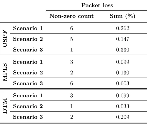
5.1.3 Packet loss . . . 56

5.1.4 Out of order packets . . . 57

5.1.5 Traffic demands . . . 58

5.2 Discussion . . . 60

Chapter 6 Conclusion 61 6.1 Project aims and achievements . . . 61

6.2 Project limitations and future work . . . 63

(9)

Appendix B Software configuration instruction 72

B.1 Controller configuration . . . 72

B.2 Network nodes and hosts configuration . . . 73

Appendix C Dynamic Topology Mechanism Source Code 80 C.1 Controller program’s source code . . . 80

C.1.1 Main program . . . 81

C.1.2 Optimisation algorithm header . . . 86

C.1.3 Optimisation algorithm . . . 87

C.2 Network nodes program’s source code . . . 95

C.2.1 Main program . . . 95

C.2.2 Initialisation and topology implementation header . . . 98

C.2.3 Initialisation and topology implementation . . . 98

C.2.4 cURL implementation header . . . 106

C.2.5 cURL implementation . . . 107

C.3 System testing program’s source code . . . 110

C.3.1 Host traffic generation . . . 110

C.3.2 Controller traffic statistic collation . . . 114

Appendix D Network performance measurements 118 D.1 OSPF baseline . . . 119

(10)

D.3 Dynamic topology mechanism . . . 127

(11)

3.1 Traffic generation during system tests . . . 19

3.2 Topology selection from traffic matrix 1 . . . 19

4.1 Logical system layout . . . 23

4.2 Physical system layout . . . 25

4.3 Flow table configuration example - Node one . . . 28

4.4 Network node software . . . 29

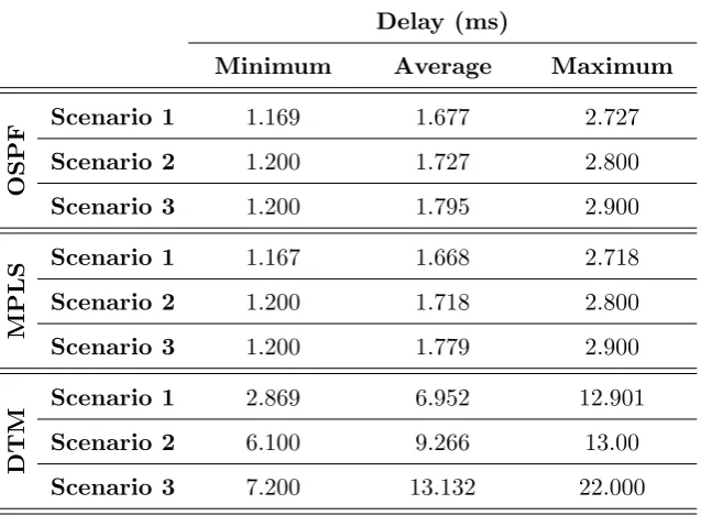
5.1 Network performance measurements — Delay . . . 54

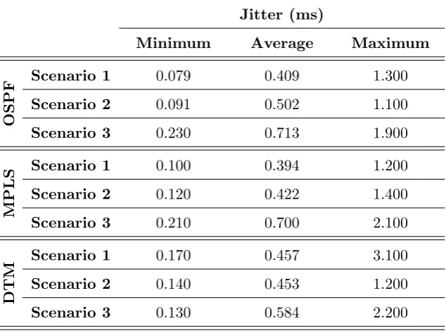
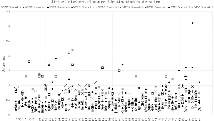
5.2 Network performance measurements — Jitter . . . 56

5.3 Network performance measurements — Packet loss . . . 57

5.4 Network performance measurements — Total demand . . . 59

(12)

2.1 Energy Aware Traffic Engineering Techniques (Coiro et al. 2013) . . . 9

3.1 Traffic matrix 1 (Mbps) . . . 18

4.1 Controller software . . . 26

4.2 Network node software . . . 27

4.3 Network host software . . . 28

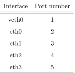
4.4 Relationship between node interfaces and Open vSwitch port numbers . . 44

5.1 Delay measurement summary . . . 54

5.2 Jitter measurement summary . . . 55

5.3 Packet loss measurement summary . . . 57

D.1 OSPF baseline — Delay (ms) . . . 119

D.2 OSPF baseline — Jitter (ms) . . . 120

(13)

D.4 OSPF baseline — Out of order packets (count) . . . 122

D.5 MPLS baseline — Delay (ms) . . . 123

D.6 MPLS baseline — Jitter (ms) . . . 124

D.7 MPLS baseline — Packet loss (%) . . . 125

D.8 MPLS baseline — Out of order packets (count) . . . 126

D.9 Dynamic topology mechanism — Delay (ms) . . . 127

D.10 Dynamic topology mechanism — Jitter (ms) . . . 128

D.11 Dynamic topology mechanism — Packet loss (%) . . . 129

D.12 Dynamic topology mechanism — Out of order packets (count) . . . 130

(14)

Introduction

The increasing focus on sustainability in modern engineering should be common knowl-edge for all engineers. Computer systems engineering is no exception, and the broad aim of this project is to reduce the energy consumption of computer networks through the use of dynamic network topologies. Telecommunications networks provide fertile ground for energy consumption improvements, as their design goals are typically limited to re-silience to link or node failure and the maintenance of services during peak periods; as a result, networks are mostly under-utilised. The periods of low utilisation can be ex-ploited to reduce energy consumption by rerouting network traffic and placing nodes and links into standby states. Dynamic network topologies can satisfy this need, with an important caveat: the traffic rerouting must facilitate reductions in energy consumption without a disproportionate degradation of network performance. The effectiveness of dy-namic topology mechanisms has been theoretically proven through simulation, with one solution reporting energy consumption reductions of 30-50% (Aldraho & Kist 2011b).

1.1

Project scope and requirements

(15)

com-putations provide a proof of concept, the use of models always contains some form of an assumption, and is therefore inherently inaccurate to some degree.

This project aims to develop a testbed that extends the previous work — mainly that of Aldraho & Kist (2011b), Aldraho & Kist (2010), and Polverini et al. (2015) — from simulation into a physical implementation. The successful development of a testbed will prove feasibility of implementation of a dynamic topology mechanism in a physical system. Furthermore, it will facilitate the measurement of the mechanism’s effects on network performance that are based on a real system, as opposed to simulated systems. This project also aims to reduce the work required for future implementations that will further develop dynamic topology mechanisms.

As stated in the project specification, which has been included as appendix A, the main requirement of the project is to use Linux’s MPLS implementation to develop and test a dynamic topology mechanism that reacts to changes in network traffic. Another project specification is the control of the network nodes’ transition between the active and standby states with the aim of decreasing total network energy consumption. Note that the node state transitions are performed by modifying the routing information, and the project does not examine the implementation of standby states. It was previously stated that network design goals favour resilience to failure and the maintenance of services during peak periods; this project does not consider the former, but preserves the latter.

The project can be divided into three main requirements: the development of the hard-ware and softhard-ware configuration of the testbed, the development of the dynamic topology mechanism programs, and the measurement of the dynamic topology mechanism’s perfor-mance. The configuration of the testbed is required to provide the capability that will be used by the dynamic topology mechanism, and the performance measurement reflects the suitability of the mechanism’s implementation in a live system. As the implementation of standby states is not examined, only the network performance is measured.

1.2

Project methodology

(16)

project begins with a review of the current literature to prevent unnecessary rework and to determine the project’s “user stories”, from which the initial specifications of the dy-namic topology mechanism testbed are be determined. After the initial research has been completed, which is detailed in chapter 2, the incremental development, experimentation, and research can commence. The development is focussed on producing functionality for the dynamic topology mechanism, and includes the development of the testbed and the dynamic topology mechanism programs. This often reveals additional functional-ity and/or component requirements, prompting additional research and experimentation prior to resuming development.

Once incremental development reaches a point where the testbed is successfully routing traffic using the dynamic topology mechanism, the focus shifts to performance validation to determine the suitability of this implementation. The performance validation is aimed at discerning the dynamic topology mechanism’s effect on network performance, and the degree to which the project requirements are met. Once the performance validation meth-ods have been developed, and the dynamic topology mechanism’s performance has been measured, the system is dismantled to prevent unpredictable use. The procedure that was used to design the system, and the resultant design itself, are detailed in chapters 3 and 4 respectively, while the testing methodology and associated results and discussion are shown in chapters 3 and 5 respectively.

1.3

Dissertation overview

This dissertation is organised as follows:

Chapter 2 analyses previous work that relates to the dynamic topology mechanism

Chapter 3 details the methodology used to develop the system and dynamic topology mechanism, and the performance validation methods used to test the resultant design

Chapter 4 fully describes the final system design, including the hardware and software configuration and the programs used to implement the dynamic topology mechanism

(17)

(18)

Related Work

There has been significant research into areas directly or indirectly related to this project, and this chapter contains a review of the current literature. The literature review details the motivation behind the project, previous implementations of dynamic topology mecha-nisms, energy aware traffic engineering, the applicability of Multi-Protocol Label Switch-ing (MPLS), topology optimisation and associated heuristics, traffic matrix calculation and measurement, and software defined networking.

2.1

Literature review

The energy consumption of the ICT sector is of significant concern; recent attention has been directed at optimising the design and use of networks and network components with consideration given to the reduction of energy consumption. The main impetus for the reduction in energy consumption of network devices is a combination of their large contribution to the ICT carbon footprint, their current inefficiency, and their role as an enabling technology for further energy consumption reductions.

2.1.1 Motivation

(19)

energy consumption of network devices is exacerbated by the almost criminally inefficient utilisation of telecommunications networks, which typically ranges from <30% (Nede-vschi et al. 2008) to <50% (Fraleigh et al. 2003); this is due to the over-provisioning of networks to maintain connectivity and Quality of Service (QoS) during peak periods, which are present for only short periods in a diurnal traffic cycle (Bolla et al. 2011). Furthermore, current network devices themselves are also inefficient, with the energy cost of data transmission at 0.128-0.225 Joules/Byte; compared to the benchmark of 802.11b radios, which use ∼1.6 µJ/B over a 100m link, the wireless link is 2-3 times more effi-cient (Gupta & Singh 2003). While the cost per byte of traffic has been decreasing due to performance improvements, the rate at which line card speeds increase has resulted in an overall increase in power density (Chabarek et al. 2008).

ICT-based low carbon technological solutions are estimated to reduce 15% of global GHG emissions by 2020, and the energy-aware focus of ICT is an attempt to secure the enabling effect of ICT in other sectors (Koenigsmayr & Neubauer 2015). Further to this, increased energy efficiency of network devices would enable greater deployment, particularly in developing countries, and allow greater network availability in the event of a disaster when power is scarce to retain data and connectivity for longer (Gupta & Singh 2003).

It is difficult to market new technologies to the carriers that maintain the internet’s core infrastructure. They have previously demonstrated satisfaction with over-provisioning, as well as techniques such as traffic caching and compression, rather than addressing the root cause (Roberts 2009). If history is any indication of the future of the internet’s core infrastructure, there will need to be a more robust solution that moves away from these temporary fixes, which can be seen as analogous to the previous use of VLSM and NAT to temporarily solve the rapidly decreasing IPv4 address space. However, in order for a solution to be widely accepted, it should align with the requirements stated in Coiro et al. (2013):

1. No new communication protocol or new functionalities in current routing and sig-nalling protocols

2. Interoperability with standard networks 3. Automatic adaptation to network condition 4. No packet loss

(20)

2.1.2 Energy consumption reduction in computer networks

The approaches to achieving the reduction in energy consumption of network devices are many and varied, and include the design of networks and network devices, link and node shutdown and standby, and traffic engineering. Most of them, if not all, either implicitly or explicitly adhere to the aforementioned requirements, as does the dynamic topology mechanism described in chapter 4.

Traffic engineering for load balancing and QoS in general

When considering the use of networks, there are several dynamic topology mechanisms that are not specifically focused on facilitating or directly influencing power consumption reduction, but which are the foundation for related works.

Traditional routing protocols, such as OSPF, support dynamic reconfiguration after topol-ogy changes. However, these are not suitable for the implementation of dynamic topolo-gies as they can take several minutes to converge (Aldraho et al. 2012). MPLS is quite versatile in terms of traffic engineering, and can provide most of the functionality of the previously used overlay model, which was implemented to address traffic engineering shortcomings of conventional IP networks, at low cost and in an integrated manner (El-walid et al. 1998, Awduche 1999). As these energy aware traffic engineering methods typically require explicit route definition, the majority of them state that MPLS must be used. However, as highlighted by Gupta & Singh (2003), consideration needs to be given to routing protocols (OSPF, EIGRP, IS-IS, RIPv2, etc.) and protocols higher in the OSI layer when testing the effectiveness of these dynamic topology mechanisms. Suryasaputra et al. (2005) demonstrates the versatility of the MPLS traffic engineering by using the NS-2 network simulator to implement explicit routing using MPLS with two different objectives: maximisation of residual link capacity, and minimisation of network cost in terms of link weights. The dynamic topology mechanism described in chapter 4 makes use of MPLS for its low cost and explicit route definition.

(21)

problem is NP hard for even a single traffic matrix, heuristics presented by Fortz & Thorup (2000) are used. Similarly, but conversely, the work of Ben Ameur et al. (2002) provides an optimal routing algorithm that routes the traffic for a pair of nodes along only one path, defined by an MPLS Label Switched Path (LSP). It uses the shortest path if possible, but also attempts to maximise the remaining capacity of the links to protect the network in the event of an increase in traffic. Kvalbein & Lysne (2007) showed an alternative use of multiple topologies that does not utilise MPLS. Their multiple topologies each have one or more links excluded to spread traffic across different paths by modifying split ratios. This method does not use explicit routing, like MPLS does, but simply distributes the traffic among several logical networks that utilise the same physical network components. This can respond quickly to traffic dynamics without requiring a demand matrix, but does not take power reductions into account.

A common aim in the use of dynamic topologies is to ensure the resilience of the network in the event of link failure. Wang et al. (2010) uses an extension of MPLS called MPLS-ff to perform reconfiguration of the network when a link failure is detected. It involves an offline precomputation phase, which takes a few seconds for a 20 node network, and an online reconfiguration phase. ICMP is used to advertise link failures across the network and traffic is then distributed among the remaining precomputed alternative links. Hundessa & Domingo-Pascual (2002) introduces a method for ensuring minimal/no packet loss during topology changes, but is focused on unplanned changes due to failures rather than traffic dependent reconfigurations. It uses pre-defined alternate LSPs for a fast switchover, and uses buffers and link failure detection to minimise packet loss. While this project does not consider network reliability and failure resilience, the concepts are still useful.

Traffic engineering for energy consumption reduction

(22)

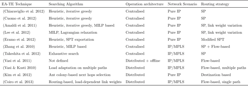
meth-ods are more direct and aim to reduce power consumption in general; Chabarek et al. (2008) proposes power awareness in the design of network devices, the allocation of those devices in the network, and the use of power aware protocols. Their definition of power aware protocols includes the use of dynamic topologies to allow network devices and/or components to move into a state with lower power consumption, and is a common area of research. Table 2.1 is derived from the work of Coiro et al. (2013), and shows an overview of a number of energy aware traffic engineering techniques. As can be seen, the majority of techniques rely on centralised control, many of them can be applied to and/or require MPLS networks, and are typically routed using a shortest path or flow-based method; Coiro et al. (2013) also proposes their own energy aware traffic engineering tech-nique that is distributed and uses MPLS. All these techtech-niques are focused on rerouting traffic to allow the maximum allowable number of links to be shutdown to reduce energy consumption, while preserving the functionality of the network as a whole.

The work of Bolla et al. (2011) also aims at reducing power consumption by rerouting traffic and shutting down unused links, but more explicitly specifies the logical connec-tion rerouting and line card shutdown methods. It uses a central entity to analyse the traffic matrix and iteratively remove the line cards with the lowest traffic load and test whether the network can still support the traffic matrix. It states that the central entity should be dedicated to collecting traffic load information and consequently applying the traffic engineering criterion to perform the virtual links’ reconfiguration while meeting QoS constraints, and that the diurnal fluctuation of traffic is the motivation behind the selection of only a few reconfiguration thresholds at 25%, 50%, and 75% of maximum demand. Yang et al. (2015) similarly aims to shut down unused line cards, but focuses specifically on the minimisation of trunk link utilisation, i.e. single logical links that are

EA-TE Technique Searching Algorithm Operation architecture Network Scenario Routing strategy (Chiaraviglio et al. 2012) Heuristic, iterative greedy Centralised Pure IP SP

(Cuomo et al. 2012) Heuristic, iterative greedy Centralised Pure IP SP

(Amaldi et al. 2011) Heuristic, iterative greedy, MILP based Centralised Pure IP SP, link weight variation (Lee et al. 2012) MILP, Lagrangian relaxation Centralised Pure IP SP, link weight variation (Eramo et al. 2012) Heuristic, SPT exportation Centralised Pure IP Modified SPT (Zhang et al. 2010) Heuristic, MILP based Centralised IP/MPLS SP + Flow-based (Takeshita et al. 2012) Exhaustive search Centralised IP/MPLS SP

(Vasi et al. 2011) Not defined Distributed + offline IP/MPLS Flow-based

[image:22.595.89.511.605.752.2]

(Vasi & Kosti 2010) Load adaptation on multiple paths Distributed IP/MPLS Flow-based, multiple paths (Kim et al. 2012) Ant colony-based next hops selection Distributed Pure IP Destination based (Coiro et al. 2013) Routing-based, load-dependent link weights Distributed IP/MPLS Flow-based, single path

(23)

comprised of several parallel physical links. By minimising trunk utilisation, less parallel links are required, and line cards can be shutdown. The proposed algorithm is distributed and uses heuristics and a hop-by-hop routing mechanism to determine the network path. The work of Pan et al. (2015) is related to the above dynamic topology mechanisms that aim to minimise the active links, as it describes an enabling technology; it proposes a modification of the line card boot sequence to drastically reduce boot time, with results in a 127.27 ms transition from the sleep to active state in their prototype hardware.

Additional techniques have been developed to expand the energy consumption reduction options to include more than just the minimisation of active links. Chu et al. (2011) presents a relatively simple method of reducing power consumption during off-peak pe-riods by using the predicted traffic matrix and topology to determine the set of routers that can be turned off while satisfying traffic demands. It then determines the explic-itly defined LSPs to reroute the traffic that would ordinarily traverse the now shutdown nodes. A variation of this discusses changes to routing decisions, based on network load, to aggregate traffic over fewer devices and links to put devices to sleep, and suggests power savings from idle components by either clocking them at a slower rate or putting them to sleep completely (Gupta & Singh 2003).

Aldraho & Kist (2011b) suggest both an energy saving method for nodes and links and a method of traffic engineering to allow its implementation, and is the main inspiration for this project. The traffic matrix is analysed with the aim of maximising the number of nodes in the a standby state. The network node standby power model is initially described by Aldraho & Kist (2010), and subsequently developed by the same authors (Aldraho & Kist 2011b, Aldraho et al. 2012, Aldraho & Kist 2011a) and others (Polverini et al. 2015, Suryasaputra et al. 2005); it proposes the temporary removal of the routing functionality, which consumes approximately 80% of a router’s energy and space (Roberts 2009). Note that when MPLS is used to facilitate the modification of topologies to support this standby mode, the MPLS-related modules must remain active to maintain labels and forwarding tables in the standby devices (Aldraho & Kist 2011a).

(24)

optimisation and control of the network, which signals the TFT and PMF on each of the network’s nodes to control the LSPs and active/standby transitions respectively. This implementation also uses timers to control the overlap period of the old and new topologies to minimise the effects on traffic. As further explored by Aldraho et al. (2012), the length of the timer has minimal impact on the power savings in the network, and is below 1% for all instances up to and including 10 power state changes in a 24 hour period for a timer value of 180 seconds.

2.1.3 Topology optimisation and traffic matrices

The solution of the optimisation problems in the vast majority of dynamic topology mechanisms involve the use of Mixed-Integer Linear Programming (MILP) solvers; the duration of the solution generation can be in the order of minutes or hours (Aldraho & Kist 2011b), and the calculation and resultant control implementation typically needs to be centralised (Gupta & Singh 2003). When testing the effectiveness of these optimised topologies, OSPF is a common benchmark, as it is widely used (Suryasaputra et al. 2005). Similarly, this project also uses OSPF routing as the benchmark of the dynamic topology mechanism’s performance measurements, as described in chapter 3.

In order to respond to the current traffic demands of the network, the optimisation meth-ods generally require an accurate traffic matrix. Traffic matrices are difficult to measure in IP networks, but Awduche (1999) shows that statistics derived from MPLS LSP tun-nels can be used to construct a rudimentary traffic matrix. Schnitter & Horneffer (2004) stated that the use of MPLS LSP statistics may not be usable for many networks as it re-quires the logical network to be fully meshed and is not scalable. However, if the nodes all perform both ingress and egress functions, as is the case in the test networks in the work of Aldraho & Kist (2011b) and in this project, the logical network is already fully meshed, and this is a suitable method to directly measure the traffic matrix. As an alternative to traffic matrix measurement, Ohsita et al. (2010) provides a method to estimate the traffic matrix using monitored link loads and the paths between source and destination nodes. This method also includes a reduction in estimation error by performing iterative calculations during the incremental reconfiguration of the network, the effectiveness of which is proven by simulation.

(25)

the optimisation problems are Non-deterministic Polynomial-time (NP) hard, so heuristics may be required for large networks to find optimal or near optimal solutions for standby node selection. Aldraho & Kist (2010) presents two such heuristics, which iteratively transitions active nodes into the standby state until the remaining active links’ utilisation becomes unacceptable, at which point it restores the latest node. The two heuristics differ in their determination of node standby priorities: the Lightest Node First (LNF) algorithm considers the node with the least connections first, while the Least Loaded Node (LLN) algorithm considers the node that handles the least traffic first. The former outperforms the latter, and the performance of both decreases sharply compared to the ILP alternative as traffic load increases. A similar heuristic is presented by Cianfrani et al. (2012), and further developed by Polverini et al. (2015), that determines the minimum number of active nodes, places the remaining ones in standby, and determines the standby nodes’ active outgoing link. It is based on the Floyd-Warshall algorithm, and can be solved for a 100 node network in approximately 25 seconds. Their algorithm always outperforms the Floyd-Warshall node standby heuristic, and is only slightly outperformed by the heuristic presented by Aldraho & Kist (2010) for networks with utilisations below 25%. However, note that this algorithm uses a different standby state that uses one outgoing link but accepts all incoming links; this is similar to the “bridged-local” state defined by Aldraho & Kist (2011b), while the work of Aldraho & Kist (2010) is based on the “bridged-all” state in the work of Aldraho & Kist (2011b). This project’s standby state is based on the aforementioned “bridged-all” state, which has been considered in the implementation of optimisation heuristics, and the heuristics themselvs are a combination of several of the aforementioned algorithms.

(26)

2.1.4 Software defined networking and virtualisation

While the physical systems that are utilised in this paper are not dedicated network de-vices, they maintain the same functionality through Software-Defined Networking (SDN) and virtualisation. As stated by Bozakov & Papadimitriou (2013, p. 196): ‘The imple-mented virtual routers are functionally and logically indistinguishable from traditional routers’. This project uses a design centered on SDN, as described in chapter 4, so the confirmation of the virtual routers’ effectiveness provides a reassuring precedence.

(27)

Methodology

The development of the dynamic topology mechanism, and the testbed on which it runs, followed a defined procedure based on agile project management concepts. This chapter describes the development methodology and the procedure used to determine the effect of the dynamic topology mechanism on network performance. The resultant system design and test results are detailed in chapter 4 and chapter 5, respectively.

3.1

Development methodology

The procedure that has been used to develop the dynamic topology testbed has been separated into the following phases: research, investigation, and experimentation; incre-mental development; performance testing; analysis; and decommissioning. The testing phase is described in the following section, the analysis phase is described in chapter 5, and the remaining phases are described below.

(28)

management and test driven development. Note that the two sub-phases described be-low were executed in parallel, as the development of the dynamic topology mechanism often presented problems that had to be solved by additional research, investigation, and experimentation. The resultant design is detailed in chapter 4.

3.1.1 Research, investigation, and experimentation

The literature review presented in chapter 2 is a product of the initial research to deter-mine the current status of work regarding dynamic topology mechanism implementation. From this, the project’s direction was determined, and an initial appraisal of the work required to achieve the project’s aims could be completed.

From the initial research, the components and capabilities required of the system could be determined. Once the physical components were selected based on the required func-tionality, experimentation and further research was performed to develop a software con-figuration for the system, such that it could support the dynamic topology mechanism.

Once an initial solution for the software configuration was determined, the incremen-tal development described below could begin. At several points during the incremenincremen-tal development, further functionality was deemed necessary; to provide a solution for the software configuration, further investigation, experimentation, and testing was performed. As such, the system’s underlying software configuration was changing almost as frequently as the dynamic topology mechanism during development.

3.1.2 Incremental development

(29)

The development of the dynamic topology mechanism was accompanied by an unsched-uled, coincidental configuration of the test network and overall system. As the develop-ment methodology also contained eledevelop-ments of test-driven developdevelop-ment, the test network to be used was a main focal point. As such, to test elements of the software, various por-tions of the network were setup and configured during development. Note, however, that full setup and configuration of the network was not performed until the dynamic topol-ogy mechanism’s development had been completed, as the finalisation of the mechanism prompted the progression to baseline determination, described below.

3.1.3 Decommissioning

Once all the required data had been measured and it was confirmed that no additional development or testing was required, the network components were dismantled to prevent unpredictable future use. The likelihood of malicious use is remote, but the precaution has be taken nonetheless. Setup and testing data has been preserved to allow replication and further analysis if necessary.

3.2

Performance validation

The system that has been developed using the above procedure must be tested to deter-mine whether it satisfies the project requirements. This testing is focussed on network performance, and can be divided into the four sub-phases described below: measurement method determination, test scenario development, baseline determination, and bench-marking. A discussion of the results of the tests, along with the results themselves, are shown in chapter 5.

3.2.1 Measurement method determination

(30)

which automatically produces a report of the connection’s jitter, packet loss, and packets received out of order, among other statistics for UDP streams. The standard ping tool can be used to provide the latency measurement. The programs used to organise the collection of these network performance data on the hosts and process it on the controller are detailed in chapter 4.

3.2.2 Test scenario development

Prior to the performance of any testing and the associated results measurement, the test scenarios first need to be determined. These scenarios are constructed to allow the collection of performance data that is easily comparable between configurations. Note that in this context, “configurations” refers to the routing mechanism being used: OSPF, MPLS, or the dynamic topology mechanism. Each of these are explained in further detail in the following sections.

As the main focus of the testing is to determine the dynamic topology mechanism’s performance when compared to conventional routing, the test scenarios are developed relative to the dynamic topology mechanism and applied to all configurations. The two key aspects that are controlled are the traffic matrices and the interval between traffic matrix changes.

(31)

Destination node

1 2 3 4 5 6 7 8 Total

Source

no

de

1 - 0.02 0.02 0.02 0.02 0.02 0.02 0.02 0.14

2 0.02 - 0.02 0.02 0.02 0.02 0.02 0.02 0.14

3 0.02 0.02 - 0.02 0.02 0.02 0.02 0.02 0.14

4 0.02 0.02 0.02 - 0.02 0.02 0.02 0.02 0.14

5 0.02 0.02 0.02 0.02 - 0.02 0.02 0.02 0.14

6 0.02 0.02 0.02 0.02 0.02 - 0.02 0.02 0.14

7 0.02 0.02 0.02 0.02 0.02 0.02 - 0.02 0.14

8 0.02 0.02 0.02 0.02 0.02 0.02 0.02 - 0.14

Total 0.14 0.14 0.14 0.14 0.14 0.14 0.14 0.14 1.12

Table 3.1: Traffic matrix 1 (Mbps)

Destination node

1 2 3 4 5 6 7 8 Total

Source

no

de

1 - 0.05 0.05 0.05 0.05 0.05 0.05 0.05 0.35

2 0.05 - 0.05 0.05 0.05 0.05 0.05 0.05 0.35

3 0.05 0.05 - 0.05 0.05 0.05 0.05 0.05 0.35

4 0.05 0.05 0.05 - 0.05 0.05 0.05 0.05 0.35

5 0.05 0.05 0.05 0.05 - 0.05 0.05 0.05 0.35

6 0.10 0.10 0.10 0.10 0.10 - 0.10 0.10 0.70

7 0.05 0.05 0.05 0.05 0.05 0.05 - 0.05 0.35

8 0.05 0.05 0.05 0.05 0.05 0.05 0.05 - 0.35

Total 0.40 0.40 0.40 0.40 0.40 0.35 0.40 0.40 3.15

Table 3.2: Traffic matrix 2 (Mbps)

Destination node

1 2 3 4 5 6 7 8 Total

Source

no

de

1 - 0.10 0.10 0.10 0.10 0.10 0.10 0.10 0.70

2 0.10 - 0.10 0.10 0.10 0.10 0.10 0.10 0.70

3 0.10 0.10 - 0.10 0.10 0.10 0.10 0.10 0.70

4 0.10 0.10 0.10 - 0.10 0.10 0.10 0.10 0.70

5 0.10 0.10 0.10 0.10 - 0.10 0.10 0.10 0.70

6 0.10 0.10 0.10 0.10 0.10 - 0.10 0.10 0.70

7 0.10 0.10 0.10 0.10 0.10 0.10 - 0.10 0.70

8 0.10 0.10 0.10 0.10 0.10 0.10 0.10 - 0.70

Total 0.70 0.70 0.70 0.70 0.70 0.70 0.70 0.70 5.60

(32)

Figure 3.1: Traffic generation during system tests

[image:32.595.89.510.75.349.2]

The traffic matrices shown in tables 3.1, 3.2, and 3.3 have been selected based on the topology selection they will elicit from the dynamic topology mechanism. The topologies that correspond to the given matrices are shown in figures 3.2, 3.3, and 3.4 below. Note that grey nodes are those that have been selected to be placed in a standby state, and which have only two active interfaces: the connection to their access network (not shown), and a connection to one active node in the network. A full description of the system’s network and the dynamic topology mechanism is provided in chapter 4, and an analysis of the traffic measurement accuracy is provided in chapter 5.

(33)

Figure 3.3: Topology selection from traffic matrix 2

Figure 3.4: Topology selection from traffic matrix 3

3.2.3 Baseline determination

This phase was concerned with the collection of data that can be used as a reference point for the dynamic topology mechanism’s performance analysis, as shown in chapter 5. To take the measurements, the system was fully setup using the test network and software configuration detailed in chapter 4. To allow a suitable comparison of the data, minimal changes were made to the underlying software between tests. The test cases that were used were based on conventional network operation: all nodes in an active state, traffic routed using OSPF; all nodes in an active state, traffic routed using MPLS with a static topology. OSPF routing was selected as it is widely used in current networks, and is frequently used as a baseline for network performance (Suryasaputra et al. 2005). MPLS was selected to isolate the effects of the dynamic topology mechanism, which also uses MPLS.

(34)

as described above.

This phase was withheld until the conclusion of the development phase. This prevents a premature collection of data that may be made unusable by a change in the underlying software configuration. Note that the conventional network operation using OSPF could have been examined very early in the project, as the required software is quite easy to configure. However, the use of a standard software configuration, i.e. one that can be used for both conventional network operation using OSPF and for network operation using the dynamic topology mechanism, allows the performance variations to be attributed to the differences in network operation, rather than differences in the underlying software configuration.

3.2.4 Benchmarking

(35)

Dynamic Topology Mechanism

and System Design

This chapter describes the final system design that is the result of the incremental de-velopment and testing outlined in chapter 3. The sections below describe a holistic view of the system, the specific hardware and software used for the controller and network nodes, and the dynamic topology mechanism’s operation. Note that the procedure used to configure the components of the system and a full listing of the dynamic topology mechanism’s source code are provided as appendix C and appendix B, respectively.

4.1

Overall system functionality and configuration

(36)

Figure 4.1: Logical system layout

simulate a local network of hosts through traffic generation and reception to and from each of the seven other access networks. The controller connected to node eight constructs a traffic matrix by monitoring the traffic between each of the node’s access networks, and uses this data to optimise the network topology. The controller then communicates the topology change to the nodes as required. Node eight was selected as the controller’s connection to the network as it is in an active state for 97% of the randomised traffic matrices applied by Aldraho & Kist (2011b). According to the same work, node 3 was never in a standby state, but was not selected as the controller’s connection as the total bandwidth of its connected links is 22 Mbps, while node 8’s total is only 12Mbps.

The hardware and software required to deliver the previously stated functionality, and to provide a foundation for the operation of the dynamic topology mechanism, is described below.

4.1.1 Hardware configuration

(37)

through node eight using its on-board Ethernet connection.

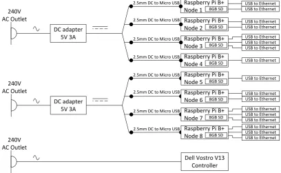
Providing power to all eight Raspberry Pis simultaneously required a moderately unique solution, and relies on a four-way split of the DC provided by two AC/DC converters. The total energy consumption of all devices at 100% CPU utilisation and all links active, using the formulae provided by Kaup et al. (2014), is approximately 34.6W, i.e. 6.92A at 5V; this is evenly divided between the two groups of nodes, nodes 1-4 and nodes 5-8. While this results in each group of four nodes drawing 3.46A at 5V — 460mA more than the rated current of the DC adapters — it is modelled on the worst case scenario and is not likely to occur. The fact that the Raspberry Pi model 1B+ requires 0.5-1W less than the Raspberry Pi model 1B on which the model was based also reduces the likelihood of this scenario occurring.

The physical devices utilised by the system are shown in figure 4.2 below, and include the following components:

• 240V AC General Purpose Outlet: Household G.P.O., provides 240V AC up to 10A

• AC/DC converter - 5V 3A: Converts the 240V AC from the G.P.O. into 5V DC with a maximum current draw of 3A, i.e. maximum current draw of 62.5mA at 240V

• 4-way DC power splitter: Splits the single 5.5mm x 2.5mm DC connector given by the DC adapter to provide four physical 5.5mm x 2.5mm DC connections

• DC power to micro USB adapter: Converts the 5.5mm x 2.5mm DC connector into a micro USB connector, which can be used to power the Raspberry Pi model 1B+

• Raspberry Pi model 1B+: Physical system that provides the functionality of a single host and node pair

• USB2.0 10/100Mbps Ethernet adapter: Provides network connectivity; the Raspberry Pi model 1B+ only has a single on-board 10/100 Ethernet port but four USB ports

(38)

• Dell Vostro V13: Physical system to provide central controller functionality. Note that this includes a proprietary AC/DC converter, not shown in figure 4.2

• Ethernet cables: Provides network connectivity between devices. Not shown in figure 4.2 for simplicity

240V AC Outlet

DC adapter 5V 3A

2.5mm DC to Micro USB

Raspberry Pi B+ Node 2 Raspberry Pi B+ Node 3 Raspberry Pi B+ Node 4

USB to Ethernet USB to Ethernet USB to Ethernet USB to Ethernet USB to Ethernet

Raspberry Pi B+ Node 1

USB to Ethernet USB to Ethernet

USB to Ethernet 2.5mm DC to Micro USB

2.5mm DC to Micro USB 2.5mm DC to Micro USB

8GB SD 8GB SD 8GB SD 8GB SD 240V AC Outlet

Dell Vostro V13 Controller 240V

AC Outlet

DC adapter 5V 3A

2.5mm DC to Micro USB 2.5mm DC to Micro USB 2.5mm DC to Micro USB 2.5mm DC to Micro USB

USB to Ethernet USB to Ethernet USB to Ethernet 8GB SD

Raspberry Pi B+

Node 5 8GB SD USB to Ethernet

USB to Ethernet USB to Ethernet 8GB SD

[image:38.595.93.502.194.445.2]

USB to Ethernet USB to Ethernet USB to Ethernet 8GB SD

Figure 4.2: Physical system layout

4.1.2 Software configuration

The software configuration is slightly more involved than the hardware configuration, particularly for the nodes and hosts running on the Raspberry Pis, but still uses readily available components. The requirements are quite specific, as the software configuration provides a foundation for the capability utilised by the dynamic topology mechanism. This section details the software configuration of the controller, nodes, and hosts. A full setup instruction to recreate the controller’s, network nodes’, and hosts’ configuration for the dynamic topology mechanism is provided as appendix B.

Controller

(39)

dynamic topology mechanism. The operating system and software packages used on the central controller are listed in table 4.1 below. Note that this is not a comprehensive list of installed software packages; the dependencies for the packages listed above, in addition to the operating system’s default packages, were also installed.

Software name Version Description

Ubuntu 14.04.2 Linux operating system.

sFlowTool 3.35 sFlow analyser. Collects sFlow messages.

NTP 1:4.2.6.p5+dfsg-3ubuntu2.14.04.3 Network Time Protocol server.

Table 4.1: Controller software

sFlowtool is used to collect the sFlow messages generated by each of the nodes, which provide information regarding the source and destination of traffic, and can be used to calculate demands between source/destination node pairs. The NTP server provides the software clock synchronisation for the nodes, as an accurate time source is a requirement to minimise network disruption during the dynamic topology mechanism’s topology changes. Note that the Quagga routing suite, which provides OSPF and other routing functionality, is not required, as the controller’s connection to node eight is used as a default gateway, and node eight advertises the controller’s network via its OSPF configuration.

Network nodes and hosts

The software that provides the required functionality for the network nodes and hosts is described below, and elaborated further in the explanation of the dynamic topology mechanism. Note that a single Raspberry Pi is configured as a network node, but also runs the network host in an LXC container, which is similar to a virtual machine running the same operating system as its host machine. The network nodes’ software is listed in table 4.2 below.

(40)

Raspbian May 2015 Linux operating system.

Quagga 0.99.22.4-1+wheezy1 BGP/OSPF/RIP routing daemon.

cURL 7.26.0-1+wheezy13 Command line tool for transferring data with URL syntax. Autoconf 2.69-1 Automatic configure script builder.

LXC 1.1.0 Userspace container object for full resource isolation and resource control. Debootstrap 1.0.48+deb7u2 Debian bootstrapper.

Open vSwitch 2.4.90 Multilayer software switch. Wondershaper 1.1a-6 Traffic shaping script.

Table 4.2: Network node software

directly, but are required to install LXC and create the LXC container that will provide the host’s functionality. The Wondershaper package is simple but vital for the emulation of Telstra network AS1221, as it applies bandwidth limitations to the inter-node links. As alluded to in the controller’s software description, NTP synchronisation is required for the network nodes, but no additional packages are required as NTP is provided by default in the listed Raspbian distribution.

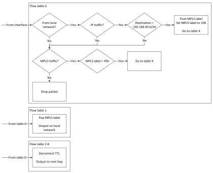
Open vSwitch is perhaps the most vital component in terms of supporting functionality for the dynamic topology mechanism, as it provides MPLS traffic processing capability that can be explicitly programmed. This multilayer switch is programmed using flow tables, which specify criteria for matching a packet, and the actions to apply to the packet once it is matched. For normal operation using OSPF, the flow tables are configured to drop all packets to prevent the generation of duplicate packets in the network. For routing using MPLS, with or without the dynamic topology mechanism, the flow tables are configured as shown in figure 4.3, and elaborated upon in section 4.4. This flow table configuration has been designed to minimise the number of flow table entries that need to be modified during topology changes. For an n-node network, then2 _{entries in table 0 are static, and}

(41)

Flow table 0

From local

network? IP traffic?

Destination = 192.168.X0.0/24

Push MPLS label Set MPLS label to 10X

Go to table X

MPLS traffic? MPLS label = Y0X Go to table X

Drop packet

Yes Yes Yes

No

Yes Yes

No No

No From interface

Flow table 1 Pop MPLS label Output on local

network From table 0

[image:41.595.88.509.93.434.2]

Flow table 2-8 Decrement TTL Output to next hop From table 0

Figure 4.3: Flow table configuration example - Node one

The hosts’ software is quite simple, as the only role they perform is traffic generation and network performance data collection. The hosts’ software configuration is shown in table 4.3 below.

Raspbian May 2015 Linux operating system.

iPerf 2.0.5+dfsg1-2 Traffic generation and measurement.

iputils-ping 3:20121221-5 Tools to test the reachability of network hosts.

Table 4.3: Network host software

(42)

which is surprisingly not installed by default. The hosts also require NTP synchronisation to control the traffic generation timing during testing, but this is controlled through the network node and automatically passed to the LXC container, so no additional software is required.

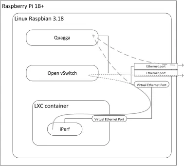
To provide insight into the purpose of the network nodes’ and hosts’ software, a dia-grammatic representation of the relationship between some of the components is shown below in figure 4.4. The grey lines represent the processing of network traffic for the host connected to the node’s access network. Communication between the host and the node is via virtual Ethernet ports, and the traffic is either processed using the routes generated by Quagga, or by the flows in Open vSwitch. Note that the packets are duplicated, so Open vSwitch must drop the packet to prevent the duplicates from reaching the network.

Raspberry Pi 1B+

Linux Raspbian 3.18

Open vSwitch

Ethernet port Ethernet port

Quagga

Virtual Ethernet Port

LXC container

Virtual Ethernet Port

[image:42.595.111.490.342.684.2]

iPerf

(43)

4.2

Dynamic topology mechanism

The dynamic topology mechanism performs functions very similar to that proposed by Al-draho & Kist (2011b), but incorporates other work (Aldraho & Kist 2010, Aldraho et al. 2012, Polverini et al. 2015) in addition to original work. The operation of the dynamic topology mechanism relies on two programs: one on the controller, and one on each of the nodes. These programs, in addition to the programs written to test the system, are explained in detail in the following sections, and outlined below:

1. Controller: Monitor network traffic

2. Controller: Optimise network topology

• Focus on energy consumption reduction through the use of router standby states

• Ensure link utilisation does not rise above a threshold value for any of the links

• Apply optimisation heuristics

3. Controller/Nodes: Communicate the topology change

4. Nodes: Implement the topology change

5. Repeat

4.3

Controller program operation

The controller’s dynamic topology mechanism program sequentially and iteratively per-forms four main functions: network traffic monitoring, traffic matrix generation, topology optimisation, and topology communication. These are each explained in detail below, along with pseudocode that corresponds to the source code that has been included as appendix C.

4.3.1 Network traffic monitoring and traffic matrix generation

(44)

data statistics for each of the 56 source/destination node pairs. The traffic data statistics are calculated by the controller program using a stream of sFlow messages. The stream is piped from sFlowTool, which collects the sFlow messages from each nodes’ instance of Open vSwitch. The command used to do so is shown below:

daniel@controller:~$ sflowtool -l | sudo ./controller

The use of the -lswitch formats the sFlow messages in the stream as comma-separated values, an example of which is shown below:

FLOW,192.168.80.1,9,4,9a3a524b5b22,fe960a04a4d4,0x0800,0,0,

192.168.80.100,192.168.10.1,17,0x00,64,37156,5001,0x00,1516,1498,32

The fields that are underlined in the above example are those used to construct the traffic matrix. These fields contain the agent IP address (i.e. reporting node’s IP address), the source and destination IP addresses of the traffic, the traffic’s packet size, and the sampling rate, respectively.

The controller program captures and analyses each sFlow message, and uses its data to determine the traffic demands of the network, which are used to directly construct the traffic matrix. The sFlow messages are captured for an interval of at least 15 seconds, which is measured to µs resolution for use in the traffic calculation. At the conclusion of the measurement interval, the traffic demands are calculated for each source/destination pair using the following formula:

Traffic demand (Mbps) = n×λ×α×8

1,000,000×τ (4.1)

In equation 4.1 above:

• n= number of samples captured during intervalτ

• λ= sampling rate (packets/sample)

• α= packet size (bytes)

• τ = measurement interval (seconds)

(45)

4.3.2 Topology optimisation

Once the traffic matrix has been constructed, the controller program can then attempt to optimise the topology with the aim of minimising the energy consumption of the network by maximising the number of nodes in the standby state. The topology optimisation algorithm is relatively simple and has been influenced by the work of Aldraho & Kist (2010) and Polverini et al. (2015). The general concept is to iteratively select a node to be placed into the standby state and calculate the predicted effect on the network links’ utilisation. If the result of placing the node in standby forces any link utilisation above a threshold value, or if any node is isolated from the network, the node is restored and optimisation is reattempted until no options remain. To allow sufficient capacity to withstand increases in network traffic and inaccuracies in traffic matrix calculation, the threshold value of 70% link utilisation has been selected. Note that the optimisation algorithm only performs calculations, and does not impact the network until the topology selection has been finalised.

As previously stated, while the optimisation is focused on reducing energy consumption, the implementation of standby states, similar to those described by Polverini et al. (2015) and Aldraho et al. (2012), and the measurement of their effect on the network has been left as future work. In this implementation, the standby state is only implemented through the modification of traffic processing, which is detailed in the explanation of the network node program’s operation.

The optimisation algorithm uses the traffic matrix and an implementation of Dijkstra’s algorithm to determine the link utilisation for a topology with all nodes active; link weights are determined using equation 4.2 below:

Link weight = 10

Link bandwidth (Mbps) (4.2)

(46)

traffic matrix and the modified topology; the topology is also examined to ensure none of the nodes have been isolated. As previously alluded to, the topology’s failure criteria are the utilisation of any of the links rising above the threshold value of 70%, or the isolation of any of the nodes from the network. If either of the failure criteria are met, the latest topology modifications are reversed and the node that was in standby is omitted from the set of standby candidates. The optimisation algorithm executes until it has attempted to place each node into standby, and the resultant topology is written to a local file to prepare it for communication and implementation.

Note that the dynamic topology mechanism can be disabled by providing any number of command line arguments to the controller’s program. Disabling the dynamic topoogy mechanism simply produces a topology configuration file that has all nodes active and uses shortest path routing. This functionality was included to enable measurement of the second baseline described in chapter 3: all nodes in an active state, traffic routed using MPLS with a static topology.

4.3.3 Topology communication

Once the optimised topology has been written to a local file, it is compared to the current topology; if there are differences between the two topologies, the oldest is overwritten, and the topology change is communicated to the nodes. The topology change is not directly communicated to the nodes, and relies on the nodes monitoring the modification time of the controller’s topology configuration file, as described in the following section. The topology configuration file contains the next hop node for each source/destination node pair, and is comprised of eight rows of eight comma-separated values; the rows signify source nodes and the fields in the rows signify destination nodes. An example of the topology configuration file’s contents is shown in listing 4.1 below.

Listing 4.1: Topology configuration file example

(47)

In the above, you can see that nodes one, four, five, and six have been placed in standby for this topology, as the next hop for all destinations is the same for a single source. Note that if the source and destination are equal, i.e. along the diagonal from top-left to bottom-right, the next hop is the current node, and the value is ignored in the nodes’ program.

After the optimised topology has been written to a local file, it is compared line-by-line with the topology file currently being used. If any line-by-line is different, the old file is overwritten, which has the appearance of updating the file contents and modification time from the nodes’ perspective, which prompts each of them to pull the new topology configuration file. The network node program operation description covers the use of the file modification times and data in further detail, but it is evident that the nodes and the controller’s software clocks must be synchronised, as previously described in the software configuration.

4.3.4 Pseudocode

The source code for the controller’s dynamic topology mechanism program is provided as appendix C, and is shown below as pseudocode for the purpose of clarity. There are two components to the controller’s program; the main program, and the optimisation algorithm.

Main program

1. Define measurement interval and topology configuration filename, and declare vari-ables

2. Initialise adjacency matrix with full topology

3. Capture measurement start time

4. Enter infinite loop

(a) Clear sFlow data from last captured message

(48)

i. Dump unwanted sFlow message fields ii. Get the node number of the message agent

A. Continue to next sFlow message capture if the node number is not one of the expected values.

iii. Dump unwanted sFlow message fields iv. Get the node number of the traffic’s source

A. Continue to next sFlow message capture if the node number is not one of the expected values.

v. Dump unwanted sFlow message fields

vi. Get the node number of the traffic’s destination

A. Continue to next sFlow message capture if the node number is not one of the expected values

vii. Dump unwanted sFlow message fields viii. Get the traffic’s packet size

ix. Dump unwanted sFlow message fields x. Get the sFlow sampling rate

(d) If the agent and destination nodes are equal, multiply the packet size by the sample rate and add it to the current traffic count for the correspond-ing source/destination pair.

(e) Measure the time difference between now and the measurement start time (f) If the time difference is greater than the measurement interval, construct the

traffic matrix and optimise the topology i. Capture a new measurement start time

ii. Use the current and previous traffic counts, the current and previous time differences, and equation 4.1 to calculate the traffic demand for every source/destination node pair

iii. Store the current traffic count and time difference as the previous traffic count and time difference

iv. Display the traffic matrix at standard output v. Create a new, empty topology configuration file

vi. Run the topology optimisation algorithm and write the output to the new file

(49)

viii. If the files are identical, delete the new file, otherwise, overwrite the old file with the new file

(g) Return to the start of the loop

Optimisation algorithm

1. Store the traffic matrix, adjacency list, output filename, and dynamic topology mechanism deactivation switch state (all passed by value from calling function)

2. Determine number of nodes in the network, initialise link utilisation threshold, and declare variables

3. Set all nodes to be active

4. Calculate shortest path for each source/destination node pair using Dijkstra’s algo-rithm

5. Use the traffic matrix and the shortest paths to determine the traffic load on each link

6. Calculate the traffic loading on each node as the sum of the traffic load on all connected links

7. Use the link traffic load and link bandwidths to calculate the link utilisation per-centage

8. Find maximum link utilisation percentage

9. If the dynamic topology mechanism is not disabled, loop while the maximum link utilisation is less than the threshold value

(a) Break the loop if attempts have been made to place each node in standby

(b) Clear the previously calculated node and link traffic loads

(c) Set the variable that tracks the reachability of the nodes to false (guarantees at least one execution of the loop below)

(d) Loop while the link utilisation is above the threshold or one or more nodes are unreachable

(50)

ii. From the set of nodes that are candidates for standby, find the node that is used as a transit node the least. Use the nodes’ traffic load to resolve any conflicts

iii. Break the loop if a least used node cannot be determined

iv. Remove the node from the set of nodes that are candidates for standby v. Store the node’s adjacency information. This is only used if placing the

node in standby has to be reversed

vi. From the set of nodes adjacent to the node to be placed in standby, find the node that is used as a transit node the most. Use the nodes’ traffic load to resolve any conflicts

vii. Update the adjacency matrix of the node to be placed in standby and all its adjacent nodes

viii. Recalculate shortest paths for new topology ix. Recalculate the traffic load on each link

x. Recalculate the link utilisation percentage xi. Find maximum link utilisation percentage xii. Test if all nodes are reachable from every node

xiii. If the link utilisation is above the threshold or one or more nodes are unreachable, reverse the actions taken to modify the adjacency matrix and return to the start of the loop

(e) Recalculate the traffic load on each link (f) Recalculate the link utilisation percentage (g) Find maximum link utilisation percentage

(h) Return to the start of the loop if the maximum link utilisation is less than the threshold value

10. Write the next hop in the shortest path for each source/destination node pair to the specified output file

4.4

Network node program operation

(51)

network is running, and iteratively checks for topology updates and implements the topol-ogy change via Open vSwitch flow table entry modifications if required. The components of the network nodes’ program are explained in detail below, along with pseudocode that corresponds to the source code that has been included as appendix C.

4.4.1 System initialisation

The system initialisation is extremely important for the operation of the dynamic topology mechanism, as it sets the foundation for the swift, synchronised reconfiguration of the network. The same program runs on all eight nodes, but with actions varying slightly for each node, so the program must first determine which node it is running on. It does this by examining the node’s hostname, which is in a standard format of “nodeX” where “X” is a digit between one and eight. Another key element is synchronisation, with all nodes using NTP to synchronise with the controller.

The final and arguably the most important action during node initialisation is the config-uration of Open vSwtich. Once it has been confirmed that Open vSwtich and the LXC container are running, or started if necessary, the MAC addresses of the LXC container’s interface and the node’s interface to the LXC container are retrieved. These MAC ad-dresses are important as they allow the flow table entries to be configured to process traffic destined for the node’s access network, i.e. destined for the access network’s host running in the LXC container. Using these MAC addresses and the node number, the Open vSwitch flows can be setup as previously described in section 4.1.2 and shown in figure 4.3. The flow table configuration can be divided into five different categories: out-put handling flow tables, firewall flows, and transit, terminating, and originating traffic processing flows, .

Originating traffic processing flows

(52)

handling flow table. The label numbering convention used in the network is quite simple, and is based on the source and destination node numbers. For example, a packet with the label “306” has originated from node three and is destined for node six. An example of a set of originating traffic processing flows for node four are shown in listing 4.2 below.

Listing 4.2: Originating traffic processing flows example (node four)

t a b l e =0 , p r i o r i t y =1000 , i n _ p o r t =1 , d l _ t y p e =0 x0800 , n w _ d s t

= 1 9 2 . 1 6 8 . 1 0 . 0 / 2 4 , a c t i o n s = p u s h _ m p l s :0 x8847 , s e t _ m p l s _ l a b e l :401 , g o t o _ t a b l e :1

In the above:

• table=0 is the first table that is examined for an entry that matches the packet

• in_port=1is the Open vSwitch port that corresponds to the node’s virtual Ethernet port connected to the LXC container

• dl_type=0x0800 matches to IP packets

• nw_dst=192.168.10.0/24 matches to a specific destination network

• push_mpls:0x8847 changes the protocol form IP to MPLS

• set_mpls_label:401sets the packet’s MPLS label value

(53)

Transit and terminating traffic processing flows

The transit and terminating traffic processing flows are identical for every node, as they simply provide a match for every possible MPLS label in the system, and define the output handling flow table to be used. A snippet of the 56 flow table entries that fall into this category are shown in listing 4.3 below.

Listing 4.3: Transit and terminating traffic processing flows snippet

...

t a b l e =0 , p r i o r i t y =500 , d l _ t y p e =0 x8847 , m p l s _ l a b e l =401 , a c t i o n s = g o t o _ t a b l e :1