Haar wavelet-based adaptive finite volume shallow water solver

This is a repository copy of Haar wavelet-based adaptive finite volume shallow water solver.

White Rose Research Online URL for this paper: http://eprints.whiterose.ac.uk/90532/

Version: Accepted Version Article:

Haleem, D.A., Kesserwani, G. and Caviedes-Voullième, D. (2015) Haar wavelet-based adaptive finite volume shallow water solver. Journal of Hydroinformatics, 17 (6). pp. 857-873. ISSN 1464-7141

https://doi.org/10.2166/hydro.2015.039

This is an author produced version of a paper subsequently published in Journal of

Hydroinformatics. Uploaded in accordance with the publisher's self-archiving policy. ©IWA Publishing 2015. The definitive peer-reviewed and edited version of this article is published in Journal of Hydroinformatics, 17 (6) 857-873, 2015 10.2166/hydro.2015.039 and is available at www.iwapublishing.com.

[email protected] https://eprints.whiterose.ac.uk/

Reuse

Unless indicated otherwise, fulltext items are protected by copyright with all rights reserved. The copyright exception in section 29 of the Copyright, Designs and Patents Act 1988 allows the making of a single copy solely for the purpose of non-commercial research or private study within the limits of fair dealing. The publisher or other rights-holder may allow further reproduction and re-use of this version - refer to the White Rose Research Online record for this item. Where records identify the publisher as the copyright holder, users can verify any specific terms of use on the publisher’s website.

Takedown

If you consider content in White Rose Research Online to be in breach of UK law, please notify us by

*Email correspondence to:  [email protected]

Haar wavelet­based adaptive finite volume shallow water 

solver

Short title: 

Dilshad A. Haleem, Georges Kesserwani* and Daniel Caviedes­Voullième

Pennine Water Group, Department of Civil & Structural Engineering, University of Sheffield, Sheffield, UK

Abstract

This  paper  presents  the  formulation  of  an  adaptive  finite  volume  model  for  the 

shallow water equations. A Godunov­type reformulation combining the Haar wavelet 

is  achieved  to  enable  solution­driven  resolution­adaptivity  (both  coarsening  and 

refinement)  by  depending  on  the  wavelet's  threshold­value.  The  ability  to  properly 

model irregular topographies and wetting/drying are transferred from the (baseline) 

finite volume uniform mesh model, with no extra notable efforts. Selected hydraulic 

tests  are  employed  to  analyze  the  performance  of  the Haar  wavelet  finite  volume 

shallow water solver considering adaptivity and practical issues including choice for 

the  threshold­value  driving  the  adaptivity,  mesh  convergence  study,  shock­  and 

wet/dry­front capturing abilities. Our findings show that Haar wavelet based adaptive 

finite  volume solutions  offer  great  potential  to  improve  the  reliability  of  multi­scale 

shallow water models.

Keywords:  finite  volume  method,  Haar  wavelets,  multiresolution,  shallow  water 

1.

Introduction

Within Computational Hydraulics, the Finite Volume (FV) Godunov­type method has 

been  extensively  used  for  modelling  shallow  water  flows  due  to  its  desirable 

properties  such  as  locality,  numerical  mass  conservation  and  ability  to  inherently 

incorporate  discontinuous  flow  transitions  within  the  numerical  solution (Bouchut, 

2007, Toro, 2001, Toro and Garcia­Navarro, 2007). 

The  original  Godunov  method  for  the  gas  dynamic  equations  assumes  that 

the  representation  of  the  numerical  solution  over  each  discrete  control  volume  is 

piecewise­constant.  Connecting  these  approximate  solutions  via  fluxes  obtained 

from the solution of Riemann Problems between cells lead to make the scheme well 

suited for solving nonlinear equations containing discontinuities (Harten et al., 1983). 

Further theoretical and numerical considerations have been given to apply Godunov­

type  FV  methods  to  shallow  water  flow  problems  in  order  to  properly  incorporate 

source  terms  (main  the  bed  slope  term)  and  model  evolving  wet/dry  fronts 

(Kesserwani, 2013, Liang and Marche, 2009, Liang and Borthwick, 2009, LeVeque 

and George, 2004). Following decades of research, FV Godunov­type methods have 

become widely applied to simulate real­scale flooding and have been adopted into 

commercial  hydraulic  modelling  software  packages  such  as  TUFLOW­FV  and 

RiverFlow2D PLUS. Nevertheless, real large scale shallow flows have complex flow 

features such as shocks, contact discontinuities and a wide range of spatial scales. 

Typically, the computational domain is discretised uniformly using a large number of 

cells,  given  that  the  position  of  flow  features  is  usually  unknown  and  capturing 

certain small scales within a coarse mesh simulation maybe difficult without causing 

to improve modelling efficiency and capture the various physical scales involved in 

shallow water flows. 

Various  adaptive  techniques  have  been  developed  within  the  FV  framework 

applied  to  solve  shallow  water  equations  (SWE).  These  include  moving  mesh 

methods (Skoula et al., 2006) or static grids with locally refinement methods (Nikolos 

and  Delis,  2009,  Caviedes­Voullième  et  al.,  2012)  .  However,  most  of  the  present 

techniques to date are achieved over patch of grid, in a decoupled manner, which 

controversially  gives  rise  to  many  problematic  effects  (Nemec  and  Aftosmis, 

2007),(Liang  et  al.,  2008,  Kesserwani  and  Liang,  2012a,  Kesserwani  and  Liang, 

2015, Mocz et al., 2013). For example they require error­sensors and multiple user­

chosen  parameters  (e.g.  for  setting  up  grid  resolution  coarsening  vs.  refinement), 

which  introduce  sensitivity  (e.g.  can  lead  to  inadequate  or  excessive  resolution), 

inflexibility and problem­dependency (e.g. due to the need to tune many parameters 

for  each  simulation  problem).  They  also  lack  a  rigorous  strategy  to  accommodate 

flow data transfer and recovery between various inner resolution scales (given the 

changing nature of the mesh). Therefore, the design of a more integrated adaptation 

approach,  which  can  address  such  problems,  is  still  a  crucial  challenge 

(Hovhannisyan et al., 2014) and is the aim of this work.

The  classical  wavelet  theory  for  local  decomposition/reconstruction  of  (self­

similar)  functions  (by  translation  and  dilatation  of  a  single  mother  function,  or 

wavelet,  at  finer  resolution)  offers  a  natural  way  for  adaptive  compression  of  data. 

Mathematicians and engineers have widely used the multi­resolution capabilities of 

wavelets in many applications (e.g. signal processing and denoising) (Gargour et al., 

2009) including the solution of partial differential equations (PDEs). The true power 

constant data can be described as a set of scaling coefficients encapsulating higher­

resolution  details  thereby  allowing  (Harten,  1995,  Keinert,  2003):  a)  genuine 

information  exchange  between  those  (heterogeneous)  elements  with  matching 

resolution  (promotion  and  demotion  of  the  details  via  application  of  high­  and  low­

pass filters), b) achievement of grid resolution adaptivity by selecting certain details 

from the local compression dataset and c) quantitatively control the variation of the 

adaptive  mesh  solution  with  reference  to  the  underlying  uniform­mesh­solution 

relevant to the finest resolution. 

In  the  context  of  the  FV  Godunov­type  modelling,  a  couple  of  papers  have 

successfully  integrated  the  wavelet  theory  for  adaptive  solution  of  homogenous 

conservation  law  (scalar  and  system)  (Harten,  1995,  Müller,  2003).  However,  the 

implementation and implication of this idea in addressing practical aspects of shallow 

water flow simulation is unexplored yet. To fulfill this gap, the Haar Wavelet basis is 

used  to  reformulate  a  FV  Godunov­type  method  to  obtain  a  new  adaptive 

multiresolution scheme, which will be referred to HWFV. The technical development 

of the HWFV solving the one dimensional (1D) SWE with source term and wetting 

and  drying  is  described.  Particular  focus  is  mainly  put  on  how  wavelet­based 

adaptivity is achieved within the HWFV SWE numerical solver. Selected test cases 

are used to systematically verify the performance of the HWFV scheme addressing 

issues of adaptivity parameterizations, modelling of irregular topography with/without 

wetting and drying, accuracy preservation and mesh convergence.

The  rest  of  the  paper  is  organized  as  follows:  Section  2  presents  a  brief 

overview  of  one  dimensional  (1D)  SWE  and  Section  3  describe  the  baseline  FV 

method  that  will  be  used.  In  Section  4,  the  multiresolution  analysis  and  its 

wavelets basis and its scaling basis are incorporated into the Godunov­type method. 

In  Section  6,  the  performance  of  the  HWFV  model  is  tested,  analyzed  and 

discussed. Section 7 draws the conclusions.

2. Shallow Water Equations (SWE)

The 1D shallow water equations considering the bed source term can be cast in a 

conservative matrix form:

•tU- •xF U S U( )? ( ) (1)

Ç È Ù É Ú ? h q U , -Ç È Ù È Ù È Ù É Ú

? 2 2

2

( ) gh q q h F U , / • Ç È Ù É Ú ? 0 x gh z S (2)

Where t is the time (s),x _{is space (m) and U, F(U) and S are the vectors containing} 

the conserved variables, the fluxes and the bed source terms respectively, in which h 

is the water depth (m), q is the flow rate per unit width _{( / )m s}2

, g is the acceleration 

gravity _{( /m s}2₎

and z is the bed elevation ( )m _.

3. Overview of the Finite Volume (FV) Godunov­type framework

In this section, the Godunov­type FV method is briefly presented (Fraccarollo et al., 

2003,  Garcia­Navarro  and  Vazquez­Cendon,  2000,  Bouchut,  2007).  The 

computational domain is divided into N0 uniform and non­overlapping cells. A cell i  

is defined as Ii ?[xi/1/ 2,xi-1/ 2] with a cell sizeF ?x xi i-1/ 2/xi/1/ 2 and a centrexi ?(xi-1/ 2-xi/1/ 2)/2

.  Integrating  equation  (1)  in  space  over  the  _ith

cell  and  time  interval _[tk_?t,tk-1_{? - Ft t]}

  yields the following conservative discrete form of the SWE:

*

+

F

- F

1

1/ 2 1/ 2 .

k k k k k

i i i

i

t t i i

t t t t

x

t

U

U

F

F

Where 

U

i

t

U   are  piecewise­constant  average  representing  the  local 

numerical solution at the present and the next time level, respectively. Fi‒1/ 2 are the 

numerical  fluxes  at  cell  interfaces,  which  are  approximated  according  to  a  two­

arguments numerical flux function, F  which is based on the approximate Riemann 

solver of Roe (Roe, 1981), and  m

i

t

S  _{includes the bed slope source term. Alternatively,} 

Eq. (3) can be rewritten in the following semi­discrete form:

-?

-

F

i i i

k k k

t t

_t

U

U

L

/

-Ã Ô

Ä Õ

Å Ö

? /

_F

/

- 

1

(

, ) ( ,

)

i i

k _{t t t t} k

i i i i

t t

i

x

L

F U U

F U U

(5)

The  techniques  adopted  for  well­balanced  discretization  of  the  bed  slope  source 

term with wetting and drying  are well­established and verified. For more details see 

(Liang and Marche, 2009, Kesserwani and Liang, 2012b, Kesserwani, 2013). Herein, 

the threshold for dry cell definition is fixed to g _?10/6

dry . The stability condition on the 

time step size (Cockburn and Shu, 2001) is controlled by a Courant­Friedrich­Lewy 

(CFL), which is chosen to be equal to 0.98 for simulations involving fully wet domains 

and 0.5 when wet/dry fronts are present. 

4.

Multiresolution analysis

In  this  section,  the  multiresolution  framework,  along  with  the  choice  of  basis 

functions  for  the  HWFV  scheme,  is  presented.  The  key  feature  of  multiresolution 

analysis  (MRA)  is  the  separation  of  the  behaviour  of  functions  at  different 

resolutions.  For  simplicity,  MRA  over  each  cell Ii  is  presented  for  the  reference 

interval [­1, 1] on which each cell is rendered. For example, any function f supported 

on a baseline interval V0 can be described on a dyadic sub­division of the baseline 

particular, this property is valid for a function space V0?

}

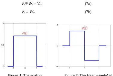
spanned by a scaling basis h (Figure 1). From the father basis h, it is possible to 

span any sub­space Vn via dilation and translation (Keinert, 2003): 

h

h _{( ) 2}? / 2 _{(2 (} - /_{1) 2 1)}/ j

n _x n n _{x j}

*

+

The  wavelet  sub­spaces  Wn  (n  ≥  0)  come  into  play  as  an  orthogonal 

complement of Vn in Vn+1 and they satisfy the conditions:

Vn¸Wn = Vn+1  (7a)

Vn ` Wn. (7b)

Figure 1: The scaling 

function at resolution n?0_. Figure 2: The Haar waveletn?0_.  at resolution 

Taking  the  Haar  wavelet {   as  a  mother  basis  that  spans W0  (Figure  2),  any  sub­

space Wn can also be spanned via its dilation and translation:

{ _{( ) 2}? / 2{_{(2 (} - / /_{1) 2 1)}

j n

n _x n _{x j}

*

+

From Eq. (6), the function f can be described in any space Vn as a linear combination 

of scaling bases hjn _{and scaling coefficients} sn_j:

l

/

? ?

 Â

0 0

n

m _{n n}

j j

n j s

This  is  called  the  single­scale  expansion  of f  at  resolution n,  where  snj  can  be  computed (or initialized) as: l / / -/ - /

-?

Ð

1 2 ( ) ( ) n

n j

n n

j _j j

s f x x dx

(10)

Due to the nested sequence of subspaces and the use of Eqs (6), (7), (8) and (10), 

an alternative expression of f can be obtained by means of the coarse description in 

V0 (i.e. at resolution n = 0) and its complementary details dnj in spaces Wn­1:

l -

_{Â Â}

0 0 _{0 0}

n

m _{n n}

j j n j

s d

f

This representation is called the multiresolution expansion of f at resolution n, where 

the detail coefficients dnj _{can be computed (or initialized) as:}

{

/

/

-/ -

/

-?

Ð

1 2

( ) ( )

n

n

j

n n

j _j j

d

f x

x dx

(12)

In the expansion (11), the representation of the function f at higher resolution (n > 0) 

is enabled by the detail coefficients  n j

d  _{when they are non­zero.}

4.1 Two scale transforming coefficients

Due to the orthonormality and the compact support properties of hjn and {jn, rigorous 

exchange of data across two resolution levels can be obtained by the so­called two 

scale transformation. To do so, two types of filter bank coefficients (a common term 

in  the  field  of  signal  processing)  are  needed.  For  simplicity,  the  two­scale 

transformation is explained for data transfer between the resolution (0) and (1). The 

first  type  of  coefficients  {k0,  k1}  is  associated  with  low­pass  filters,  i.e. Eq  (13); 

whereas the second type of coefficients {g0, g1} is associated with high­pass filters, 

i.e. Eqs. (14):

h h h h

/

? 0 1 ?

_Ð

h h h h

? 0 1 ?

_Ð

1 0, 1 ₀ 0( ) ( )x 1 x dx

k   _(13b)

h { h {

/

? 0 1 ?

_Ð

g x x dx _(14a)

h { h {

? 0 1 ?

_Ð

g x x dx _(14b)

Low­pass filter coefficients {k0, k1} are used to merge the two scaling coefficients at 

resolution  (1)  into  one  scaling  coefficient  at  resolution  (0),  (this  is  referred  to  as 

demoting):

?

-0 1 1

0    0 0    1 1

S k S k S _(15a)

High­pass  filter  coefficients  {g0,  g1}  are  used  to  obtain  (or  actually  store)  the 

complement details (or detail coefficients) of the scaling coefficients at resolution (1) 

in resolution (0):

?

-0 1 1

0   0 0   1 1

d g S g S _(15b)

Combined use of both filter coefficients allow to compute the scaling coefficients at 

resolution  (1)  from  the  scaling  coefficients  at  resolution  (0)  and  their  (stored) 

complement detail coefficients (this is referred to as promoting):

-?

1 0 0

0

S k S g d _(16a)

?

-1 0 0

1    1 0      1 0

S k S g d _(16b)

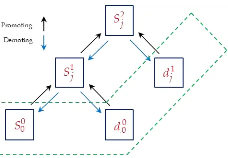
By  recursive  application  of  the  two­scale  transform  equations,  the  expansion  of 

scaling coefficients describing a function f can be demoted or promoted across any 

different  resolutions  (Figure  3).  Consequently,  promoting  and  demoting  the 

coefficients  across  different  resolutions,  i.e.  by  using  the  Eq.  (15)  and  (16),  is  the 

Figure 3: The promoting and demoting of the scaling coefficients numerical solution 

across different resolutions

5. Haar Wavelets Finite Volume method (HWFV)

This section shows how to exploit the multi­resolution description of function f (recall 

Section 4) to decompose the local piecewise­constant solution Ui (recall Section 3) 

as a compressed dataset of the solution’s information, which drives adaptivity. The 

strategy  is  to  first  generate  a  FV  discretization  at  the  highest  resolution  (herein 

presented  for n  =  2  without  loss  of  generality)  to  produce  a  fine­uniform­reference 

mesh. Then, over this mesh, MRA is performed to select up to which resolution the 

local  numerical  solution  needs  to  be  described  (i.e.  form  a  heterogeneous  grid  for 

actual  FV  calculations).  In  doing  so,  three  main  steps  are  needed:  prediction  for 

careful mesh refinement, multi­resolution FV update and thresholding step for mesh 

coarsening through solution decompression.

5.1 Multi­resolution FV formulation 

Following  to  the  discretization  presented  in  Section  3,  a  higher  resolution  mesh  is 

introduced.  Each  cell  of  the  baseline  coarse  mesh,  i.e.  presented  in  Section  3,  is 

spatial  resolution  _{F ?x}n ₂/n_Fx

.  A  sub­cell  centre  is  denoted  by  xni j, ?xi/1/ 2-Fxn(j-1/ 2) 

? /

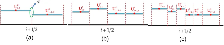
(j 0,1,...,2n 1)_{.  Figure  4  shows  the  multiresolution  stencil.  In  this  multiresolution} 

setting, the FV formulation, described in Eqs. (4) and (5), can be rewritten as: 

-? -F

1

, k , k ,

i j i j i j

n t n t _tLn

U

U

/ -/ -Ã Ô Ä Õ Ä Õ Å Ö ? / /

F

-

1 1

. . 2 2  ( 1. , . ) ( . , 1.)

i i n i j i i i Roe Roe

i j i j i j i j i j _I

n _{n n}

n n

n

x

F

F

S

L

(18)

Here the translating index j is related to the resolution level of the local cell n. 

 Figure 4. Local multiresolution stencil {Ii jn, } embedded within cell I_i.

Eqs.  (17)  and  (18)  need  to  be  only  applied  at  a  local  level  resolution  (i.e.  on  the 

adaptive mesh). This mesh can be selected by, first, casting each local solution as in 

Eq.  (11).  This  requires  demoting  high­resolution  data  in  order  to  store  detail 

coefficients and produce the scaling coefficient at level (0). Then, a mesh prediction 

step is needed to locally promote the solution and refine the grid. This will yield the 

performed to reduce the density of the mesh by discarding all non­significant details 

that fall below a certain threshold­value (details in the sections below).

5.2. Prediction step for mesh refinement 

Since the flow field is evolving in time, the prediction step must be performed after 

each  time  step  to  guarantee  no  significant  features  of  the  numerical  solution  are 

omitted  in  the  next  time  step.  The  prediction  strategy  is  only  based  on  the 

information  available  at  the  current  time  level  (Müller,  2003,  Müller  and  Stiriba, 

2007). Generally, the detail coefficients of predicted cells are not available. Thus, the 

local  solution  over  the  predicted  cells  is  promoted  by  simply  setting  zero  detail 

coefficients  (Harten,  1995).  To  do  this,  the  following  algorithm  is  used  to  identify 

those neighbourhood cells that needs to be further refined:

a) Find the scale coefficients of the conserved variables at leveln?0. 

b) Compute the normalized gradient c  between the local cell and its neighbour 

cell (see Figure 5a).

c? /

-0 0 ,0 1,0

0 ,0

max(1, )

i i

i

U U

U ₍₁₉₎

c) Introduce two indicators to compare c values and decide the resolution levels 

of neighbouring cells that have significant details. Here, the values of c ? 0.1 

and  c ?0.05  are  chosen  as  indicators  for  all  numerical  test  cases.  The 

decision for the local refinement mesh will take the following form according to 

the  value  of  c .  If  c 0.1  _{the  adaptive  mesh  is  as  in  Figure  5(c).  If} 

c

@

(a) _{(b) (c)}

Figure 5:  Mesh prediction cases

5.3. Thresholding step for the decompression of mesh

Thresholding is applied on the detail coefficients after each update to decompress 

the mesh. The values of detail coefficients (Dni j, ) become small when the numerical 

solution is smooth. Therefore, they can be cancelled without substantially affecting 

the  accuracy  of  the  numerical  solution.  To  do  so,  all  detail  coefficients  whose 

absolute  values  are  below  a  normalised  level­dependent  threshold  value  are 

discarded, i.e. if they satisfy 

g

/

> .

.

2 max(max ,1)

i j

i j

m n

n

n

D

U ₍₂₀₎

The  components  in  Dni j,   are  associated  with  the  components  of  the  conserved 

variables  in  Uni j,   (i.e. h  and q).  In  real  computations,  it  is  impossible  to  know  the 

optimal threshold value but a range of options is feasible (Hovhannisyan et al., 2014, 

Gerhard and Müller, 2013) as will be investigated in the following section. By default, 

in  this  work,  the  threshold­value  (at  the  coarsest  level)  is  set  to g?0.01  _{and  it  is} 

normalized  according  to  the  resolution  levels.  In  addition,  the  magnitudes  of  the 

detail  coefficients  are  scaled  according  to  the  maximum  value  of  the  numerical 

solution. 

The topography is projected into the highest resolution (n = 2) in the same way as 

the conserved variables. Thus the compressed dataset of bed information over each 

cell  is  obtained.  Finally,  the  adaptive  bed  mesh  is  obtained  by  applying  the 

thresholding  step.  But  the  topography  adaptation  is  performed  once  (i.e.  initially 

when  t?_{0)  and  it  remains  constant  throughout  the  simulation  time.  To  ensure  the} 

preservation of an accurate water surface elevation and mass conservation across 

levels,  the  bed  mesh  should  be  considered  as  a  reference,  this  means  that  the 

HWFV scheme does not allow demoting the local numerical solution to coarsen the 

mesh  to  a  resolution  level  lower  than  the  topography  refinement,  even  if  the  local 

numerical solution allows for a lower refinement level. 

6. Numerical results 

This section shows the ability of the new HWFV scheme to solve 1D shallow water 

problems  with  fewer  cells  when  comparing  to  the  reference  FV  scheme,  while 

retaining  accuracy,  total  mass  in  the  system,  well­balancing  and  positivity  of  water 

depth. Five well­known benchmark problems are considered for validation of HWFV 

scheme. Furthermore the Root Mean Square Error (RMSE) and the Relative Mass 

Error  (RME)  are  computed.  Two  of  the  test  cases  are  idealized  dam­break  cases 

over frictionless beds (regular and irregular), the third and fourth test cases consider 

steady flow over a hump (transcritical flow with shock and supercritical flow) and the 

fifth test case considers a deeper analysis on the test case of the oscillatory flow in a 

parabolic bowl. 

The purpose of this case is to test the capability of the HWFV scheme to efficiently 

and  accurately  solve  the  homogenous  shallow  water  equations.  The  solution  is 

compared to the exact solution, using the Root Mean Square Error (RMSE) and the 

maximum  error  metrics.  A  1D  channel  with  a  horizontal  frictionless  bed  is 

considered. The length of the channel is 2000m _{and an imaginary dam is located at} 

1000 m from the upstream end. Initially, the upstream water level is 20 m whereas 

at the downstream end, the water level is 5.0m_{. The initial discharge was set to zero} 

in every cell. Boundary conditions, although set to be numerically transmissive, are 

effectively  irrelevant  in  this  case  as  the  propagating  wave  does  not  reach  the 

boundary. At the instant of dam failure, water is released producing a shock wave 

travelling  downstream  meanwhile  a  rarefaction  wave  is  formed  propagating 

upstream. The computational domain at the coarse level (n = 0) is discretised with 71 

uniform cells and the computational model was run up to 40 second after the dam 

break. Since the HWFV model allows for up to 3 levels of mesh refinement, the size 

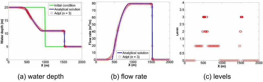
of the reference fine uniform mesh is 568 cells. The numerical results are illustrated 

in Figure 6. The highest level of resolution is noted to be reached at the shock wave 

and the kink at the tail of the rarefaction wave. The other zones of the rarefaction 

wave are achieved with the intermediate resolution levels 1 and 2. Meanwhile, at the 

rest  of  the  domain,  where  the  solution  is  smooth,  the  HWFV  has  retained  the 

baseline coarse level. In this test, the adaptive solution required a maximum of 124 

(a) water depth (b) flow rate (c) levels Figure 6: HWFV adaptive numerical solution to the idealized dam break flow Further quantitative analysis is performed via calculating the RMSE for both  water surface and flow rate, i.e.: 

*

+

ÂÂ Â

0 2 1 2 , , 1 0 0

ˆ n

N m

i j i j

i j n n n h h h RMSE AC (21)

*

+

ÂÂ Â

0 2 1 ₂

, , 1 0 0

ˆ n

N m

i j i j

i j n n n q q q RMSE AC (22)

In which  ACis the total number of active cells forming the adaptive mesh, hi jn, ,qi jn,  

are  the  numerical  results  and  hˆi jn, _,ˆi j,

n

q

  are  the  reference  data  (from  the  analytical 

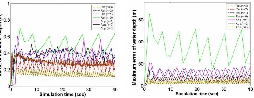
solutions).  Figure  7  and  Figure  8  compare  the  depth's  RMSEs  and  Maximum 

absolute errors (in L­infinity norm), respectively, for the different uniform and adaptive 

meshes considering up to a maximum resolution level of n = 3. Clearly, both error 

profiles  show  a  decrease  in  error  magnitude  with  an  increase  in  baseline  mesh 

resolution, which is expected due to grid convergence properties. The variations of 

the  RMSEs  resulting  from  the  adaptive  HWFV  models  are  bounded  between  the 

RMSEs  obtained  from  the  coarsest  baseline  uniform  mesh  model  and  the  finest 

uniform mesh models. Such bounding of the adaptive RSMEs is expected because 

an adaptive mesh scheme at a resolution n is set to further allow lower resolution 

down  to  the  baseline  resolution  0.  However,  since  the  maximum  depth  errors  are 

governed  by  the  highest  resolution  (due  to  shock  presence),  their  error  trends  are 

resolution n shows comparable error range to the reference uniform counterpart and 

(ii) the variation of the adaptive errors are consistent level­wise. In addition, a more 

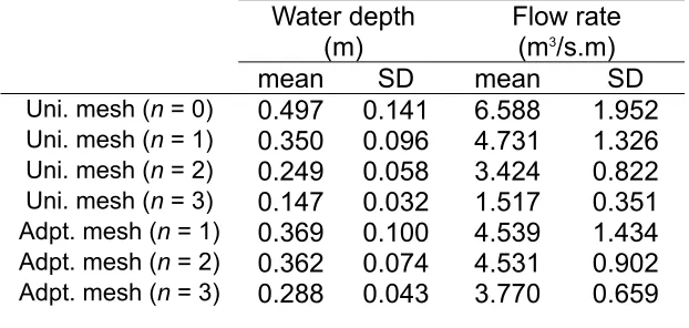
quantitative  analysis  is  considered  via  tabulating  the  mean  and  standard  deviation 

(SD)  of  the  RMSEs  (see  Table  1).  These  results  show  decreasing  trend  for  the 

means  accompanied  by  a  faster  reduction  in  their  SDs  with  more  profound 

refinement levels in adaptive scheme. Therefore, the HWFV framework performs the 

adaptivity process without introducing any additional errors to the numerical solution 

and is able to sensibly decide resolution level in track with the dynamics of the flow. 

For this test, the adaptive model simulation cost around 78 % less, in computational 

efforts, than the simulation on the finest uniform mesh. 

In the following test cases, the highest level will be fixed to n = 2 and the focus 

will be put on exploring applied aspects that are relevant to hydraulic modelling. 

Figure 7: RMSE evolution for the dam­

break case.

Figure 8: Max error evolution for the dam­

Table 1: The mean and standard deviation of RMSE for Dam­break test case

Water depth 

(m) Flow rate (m3_/s.m)

mean SD mean SD

Uni. mesh (n = 0) 0.497 0.141 6.588 1.952

Uni. mesh (n = 1) 0.350 0.096 4.731 1.326

Uni. mesh (n = 2) 0.249 0.058 3.424 0.822

Uni. mesh (n = 3) 0.147 0.032 1.517 0.351

Adpt. mesh (n = 1) 0.369 0.100 4.539 1.434

Adpt. mesh (n = 2) 0.362 0.074 4.531 0.902

Adpt. mesh (n = 3) 0.288 0.043 3.770 0.659

6.2. Steady flow over a hump

This case is employed to test the performance of the current scheme in reproducing 

a steady flow over non­uniform topography in a frictionless rectangular channel 1m 

wide  and  a  25m  long.  The  analytical  solution  was  supplied  by  Goutal  and  Maurel 

(Goutal and Maurel, 1997) and the bed reads:

Ê / /

Í ? Ë ÍÌ

2

0.2 0.05( 10) 8 12 0

b x x

z

otherwise ₍₂₃₎

6.2.1. Transcritical case involving shock

The initial water surface and flow rate per unit width are set to h + z = 0.33 m and q = 

0.18  m2/s,  respectively.  Physical  boundary  conditions  consisted  of  the  steady 

discharge at the inflow and the initial water level at the outflow. The coarse baseline 

mesh comprised 50 uniform cells and simulations are noted to converge at around t 

= 170s. For this test, the adaptive HWFV model has been further implemented and 

assessed along with the upwind discretisation of the source term (Vázquez­Cendón, 

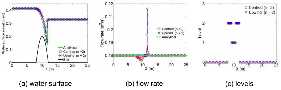
1999).  Figure 9 presents the numerical results of the adaptive scheme (with n = 2) 

as compared to the analytical solutions. The numerical water surface profile shows a 

very  good  agreement  with  the  analytical  solution  for  both  the  upwind  and  the 

rate, it seems to be typically improved by the upwind source term discretization apart 

from the peak caused by the presence of the water jump. Arguably, this is a known 

deficiency in standard finite volume schemes and, thus, does not relate the proposed 

wavelet­based  adaptivity  (Garcia­Navarro  and  Vazquez­Cendon,  2000,  Toro  and 

Garcia­Navarro,  2007)).  In  this  case,  the  majority  of  the  domain  features  required 

coarse resolution level except at the hump, which dictated local level 1 of refinement 

from  the  onset  and  at  the  discontinuities  (i.e.  starting  kink  of  the  transcritical 

transition and shock) where the level was refined to highest.

(a) water surface (b) flow rate (c) levels

Figure 9: HWFV adaptive numerical solution for the steady transcritical flow over a hump.

6.2.2 Supercritical flow case

In order to ensure that the disturbances observed in the discharge in the previous 

test case (Figure 9) are not induced by adaptivity over the local cells (see Section 4), 

the supercritical flow case over hump is also considered. Channel geometry and bed 

topography  are  identical  to  the  previous  test  case,  but  the  unit  inflow  rate  and 

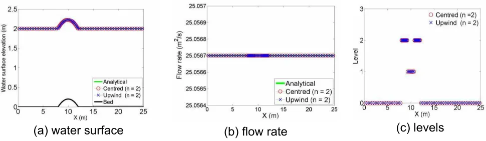
elevation water surface at the upstream of the channel are set to h + z = 2 m and q = 

25.0567 m2/s, respectively. Herein, both of these physical values are used as steady 

state  inflow  boundary  conditions;  whereas  a  free  outlet  is  numerically  set.  The 

results  are  shown  in  Figure  10.  The  constant  flow  rate  and  surface  water  profile 

compared with the analytical solution are well captured. Again, the mesh refinement 

was  obtained  only  in  the  regions  where  both  bed  elevation  and  flow  are  varying. 

However,  no  artefacts  are  noted  in  the  prediction  of  the  discharge  for  both  the 

upwind  and  cell­centred  discretisation.  Consequently,  the  two  test  cases 

demonstrate  the  good  performance  of  the  adaptive  shallow  water  flow  model  in 

reproducing well­balanced steady flows over topography, and in performing selection 

of resolution levels in relevance with flow and topographic regions.

(a) water surface (b) flow rate (c) levels Figure 10: HWFV adaptive numerical solution for the suppercritical flow over a hump.

6.3. Dam­break over over a triangular hump

This  test  case  is  employed  to  verify  the  capability  of  HWFV  to  preserve  the  total 

mass in the system in order to ensure that the adaptivity process does not introduce 

or lose mass even in the presence of shocks and wet/dry fronts. A hypothetical dam 

Figure: 11 Dam break over a triangular hump

The  length  of  the  horizontal  flume  is  38m  _{and  a  dam  is  located  at  15.5} m 

from  the  upstream  end.  A  reservoir  with  a  water  surface  elevation  of  0.75m  is 

located upstream from the dam and the rest of the domain is dry. Mesh resolution at 

the coarse level consisted of 13 cells. Reflective boundary conditions are set at the 

both ends of the channel. At t = 0 s the dam is assumed to fail causing violent wave 

propagation;  namely,  the  wetting  front  rushes  into  the  floodplain,  overtops  and 

interacts with the obstacle creating a reflected­wave that will again be reflected by 

the boundary walls. Since the system is closed, the initial mass of water should be 

conserved. During the simulation, the total mass of water at time t (M.t) is computed 

and  compared  with  the  total  initial  discrete  mass  (M,0)  according  to  the Relative 

Mass Error (RME) below:

/ ? , 0

0 R_ME Mt M

M   ₍₂₄₎

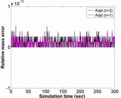
The results in Figure 12 show that the adaptive HWFV models conserve the initial 

total mass in the system and the magnitude of RME is within the range of machine 

precision  (_{1 10·} /15_{)  throughout  the  entire  computational  time.  However,  since  in  the} 

HWFV scheme the mesh resolution is not fixed, the real physical mass (M,R) is also 

used, as a reference, to show the ability of HWFV to preserve the same amount of 

mass  as  compared  to  the  corresponding  uniform  mesh  size;  this  has  been  done 

according to the Eq. (25) below:

/ ?

R t R

R M M ME

M ₍₂₅₎

In  Figure  13,  the  results  show  that  the  RME  profiles  for  both  the  adaptive  mesh 

not introducing any additional mass error beyond the capability of the discretization 

relative to the fine reference uniform scheme.

Figure 12: RME evolution for dam break 

over a triangular hump (compared with 

the projected mass t = 0).

Figure 13: RME evolution for dam break 

over a triangular hump (compared with the 

physical real mass)

6.4. Oscillatory flow in a parabolic bowl 

This  case  is  well  known  and  recognised  as  a  challenging  test  case  for  numerical 

models  because  it  involves  both  moving  wet/dry  interfaces  and  it  has  an  uneven 

topography. It is selected here to study accuracy and mesh convergence abilities of 

the adaptive HWFV scheme and to explore the sensitivity of the HWFV model, i.e. in 

performing  the  adaptivity  process,  considering  various  choices  for  the  threshold­

value parameter and for the baseline coarsest mesh.

The  bed  is  described  by  z x h x a( )? 0

* +

consists  of  an  oscillatory  flow  taking  place  inside  a  parabolic  bowl.  The  transient 

analytical solution was proposed by Thacker (Thacker, 1981): 

j( , )? 0/ 2cos(2 )/ 2 / cos( )

4 4

B B x

x t h st Bs st

?

( , ) sin(2 )

u x t B st ₍₂₇₎

where  B?  5  is  a  constant  value  and  s?1 2 8a gh0   _{is  the  frequency.  Under  these} 

conditions  the  oscillation  period  is  T?_{1345.94s.  The  case  was  simulated  on  the} 

domain [­5000m; 5000m] using different computational mesh cells at coarse level (

0

N _{). Simulations were run up to 1.5}T_{. Boundary conditions are irrelevant because} 

the flow never reaches the boundaries. They were set as transmissive boundaries. 

6.4.1 Threshold sensitivity 

To understand the effect of the threshold value parameter on the adaptivity process, 

a baseline mesh with N0? 40 cells is fixed, while considering the following threshold 

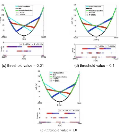
values: g? 0.0, 0.001, 0.01, 0.1 and 1.0. In Figure 14, the numerical water surface 

profiles  at  t?  _{275s  (}T/ 5_{)  and}  t?_{2020s  (1.5}T )  are  compared  with  the  analytical 

solution. As seen in the figure, the HWFV scheme refines in the region where the 

wet/dry interface is moving through. Meanwhile, other parts of the domain stay at the 

coarsest and the intermediate levels of refinement. Furthermore, it can be seen that 

varying the threshold value leads to different refinement patterns. In particular it is 

shown  that,  as  g  _{increases  fewer  cells  are  refined  to  higher  levels  during  the} 

simulation, since smaller detail coefficients are selectively omitted. In Figure 14(a), it 

is clear that the adaptive HWFV scheme activates all the details coefficients when 

g?  _{0.0  and  all  the  computational  cells  go  to  the  highest  level,  thus  resulting  in  a} 

uniform  mesh.  Figure  14(b)  shows  an  almost  uniform  mesh  prediction  when  g?

0.001. Hence, it is not reasonable, in terms of efficiency, to use a threshold value g> 

0.001. A sensible refinement is obtained with g?0.01 (Figure 14(c)). For g? 0.1 and 

g?_{1.0  (shown  in  Figure  14(d­e)  respectively)  poor  predictions  at  the  wet/dry} 

leads to omit some small detail coefficients, relevant to the wet/dry front, during the 

6.4.2 Baseline meshes.

The choice of a baseline mesh with N0? 40 is rather arbitrary, and it might be already 

too fine, or on the contrary, never allow for a fine enough mesh for this test case. 

This may affect the performance of the adaptivity process. Therefore, the influence 

of  the  baseline  mesh  should  be  studied.  Several  baseline  meshes  at  coarse  level 

?

0

N  _{20, 40, 80,160 and 320 are introduced to address this. The same settings of the} 

threshold value as reported in Figure 14 are used. The evolution of the number of 

active  cells  is  presented  in  Figure  15.  The  results  confirm  that  all  considered 

combinations of N0and g are able to perform the adaptive solutions. Moreover, when 

refining the baseline mesh, the HWFV requires a reduction of the threshold value to 

better perform adaptivity process. This is due to the fact that most of the flow region 

results  in  rather  smooth  solutions;  therefore  the  value  of  the  detail  coefficients  is 

small. In Figure 15, N N/ 0 reduces as the baseline mesh is refined, regardless of the 

varying threshold. However, in Figure 15 (d­e) for g?0.1 and g?1.0, the magnitude of 

0

/

N N  _{is relatively the same and with values bounded between 1.0 and around 2.5.} 

These values are less when compared to other threshold values, but they strongly 

influence the quality of the numerical solution. Notably, with g? 0.01, regardless of 

0

N _{, optimal results are obtained, in comparison to other threshold values. The value} 

of  N N/ 0is  bounded  between  around  1  to  4.  This  case  shows  a  particular  trend  of 

how the pattern of active cells varies withN0. This trend indicates that g? 0.01 is the 

most  sensitive  toN0.  Because  of  this  sensitivity,  this  threshold  value  allows  for  a 

wide, automatic response of the adaptive process (contrary, to, for example g?0.1) 

and therefore is likely to be the best to perform adaptivity in a prompt way. It is clear 

that an inefficient adaptive process is obtained with g? _{0.001 except in Figure 15(e),} 

6.4.3. Mesh convergence 

Mesh  convergence  is  also  studied  in  terms  of  the  _L1_{­norm  as  defined  in  Eq.  (28).} 

Simulations were performed up to 2020 s and for analysis the t?_{270s (T/5) and} t?

2020s (1.5T) are selected. Several baseline meshes at coarse level N0? 10, 20, 30, 

40, 80,160 and 320 are introduced with using the same threshold values as defined 

previously.  It  can  be  seen  in  Figure  16  that  the  behaviour  of  the  _L1_{­norm  is} 

asymptotic  regardless  of  N0  and  g.  The  uniform  mesh  (g?0.0)  is  taken  as  a 

reference curve for comparison. Each point within a curve is associated with each 

baseline mesh. The difference between the convergence curve for g? 0.001 and the 

reference are relatively small. For g ? 0.01 the convergence is slightly better than all  as shown in Figure 16 (a) and Figure 16(b). The large error obtained with g? _1.0 and 

?

0

N  _{20, 30 cells and this is due to too few cells being activated during the adaptivity} 

process  (over­filtering).  Thus  the  quality  of  the  numerical  solution  is  affected. 

Nevertheless, the magnitude of the error becomes smaller as N0 increases but still 

remains larger than the error of the reference curve. Furthermore, the better results 

are  obtained  for  g?  _{0.1  but  with  sensible  differences  compared  to}  g?  _{1.0.  The} 

magnitude  of  the  _L1_{­norm  is  increased  from  Figure  16(a)  to  Figure  16(b).  This  is} 

merely because of numerical diffusion which is an anticipated issue for finite volume 

first­order schemes. In Figure 17, the same analysis, as the one reported in Figure 

16,  is  considered  to  illustrate  the Relative Performance  of  CPU  time  (RPCPU). 

Figure 17(a) shows the ratio of the CPU times of the adaptive schemes to the CPU 

time obtain from the associated fine uniform reference schemes (i.e. g? 0.0); while 

Figure  17(b)  further  describes  the  normalised  CPU  times,  which  are  obtained  by 

clearly  that  when g @  0.0,  less  time  is  required  for  achieving  a  simulation  as  the  baseline  mesh N0 density  increases.  They  also  show  that  the  efficiency  of  the 

adaptive HWFV schemes is near their equivalent uniform mesh FV schemes when 

the baseline mesh has a size N0 ≤ 40 and despite the choice of g. 

For g = _{0.001 the RPCPU and normalised CPU time are noted to be inefficient} 

despite the choice of the baseline mesh N0. In contrast, for g = 0.01, 0.1 and 1.0 they 

start  to  significantly  decrease  in  proportion  with  an  increase  in  the  density  of  the 

baseline mesh N0. However, for g = 0.1 and 1.0 the RPCPU tend to remain close for 

N0 ≥ 40; whereas, with g = 0.01 the RPCPU showed consistent decrease in line with 

the refinement of the baseline mesh N0; this suggest that a threshold value of g = 

0.01 enables best selection among the magnitude of the detail coefficients, and so 

allows optimal efficiency and accuracy in the context of the proposed HWFV model 

for a baseline mesh of around 40­100 cells. 

*

+

/

? ? ?

/

?

ÂÂ Â

1

, , , 1 0 0

ˆ ­norm

n

N m

i j i j i j

i j

n n n

n dx h h

L

(28)

(c) threshold value = 0.01 (d) threshold value = 0.1

(e) threshold value = 1.0

Figure 14: numerical solution against the analytical solution in parabolic bowl flow (

?

0

N _{40), considering different threshold values.}

(c) N0? 80 (d) N0? 160

(e) N0? 320

Figure 15: time evolution of active cells for various baseline meshes in parabolic 

(a) t?₂₇₀s

(b) t?₂₀₂₀s

Figure 16: Comparisons of _L1_{­norm for parabolic bowl. Each highlight point is} 

(a) (b)

Figure 17: Comparisons of the relative CPU time for parabolic bowl

7. Conclusions

Adaptive  mesh  refinement  schemes  are  useful  tools  to  efficiently  model  various 

scales  of  shallow  water  flow.  A  new  adaptive  formulation  is  proposed,  which 

combines  the  Haar  wavelets  with  the  FV  method  (HWFV).  The  appeal  of  the 

formulation  can  be  easily  exploited  to  drive  spatial  resolution  adaptation  from  the 

solution  itself  according  to  a  single  threshold  value  .  A  series  of  numerical  tests 

have been performed, considering issues of well­balanced property, convergence of 

scheme, sensitivity relating to different choice of the thresholds values and ability to 

treat wet/dry fronts. 

Numerical evidence confirms that the proposed HWFV scheme can accurately solve 

the shallow water equations with source term. Adaptive solutions are shown to be 

mass  conservative.  Notably,  the  new  model  is  proven  to  be  able  to  self­decide 

appropriate  resolution  levels  following  the  dynamics  of  the  flow,  including  shocks, 

of integrating the friction source term in a well­balanced manner, exploring sensitivity 

issues in relation of increasing the resolution levels with varying threshold values and 

extending the approach to 2D.

Acknowledgments

The  first  author  acknowledges  the  support  of  the  Kurdistan  Regional  Government, 

ministry of high education and scientific research. The research is further supported 

by  the  UK  Engineering  and  Physical  Sciences  Research  Council  (grant  ID: 

EP/K031023/1)  and  by  the  Pennine  Water  Group  platform  grant  (grant  ID: 

References

Bouchut,  F.  2007.  Efficient  numerical  finite  volume  schemes  for  shallow  water  models. 

Edited Series on Advances in Nonlinear Science and Complexity, 2, 189­256.

Caviedes­Voullième, D., García­Navarro, P. & Murillo, J. 2012. Influence of mesh structure  on  2D  full  shallow  water  equations  and  SCS  Curve  Number  simulation  of  rainfall/runoff events. Journal of Hydrology, 448–449, 39­59.

Cockburn,  B.  &  Shu,  C.­W.  2001.  Runge–Kutta  discontinuous  Galerkin  methods  for  convection­dominated problems. Journal of scientific computing, 16, 173­261.

Fraccarollo,  L.,  Capart,  H.  &  Zech,  Y.  2003.  A  Godunov  method  for  the  computation  of  erosional  shallow  water  transients. International  journal  for  Numerical  Methods  in  fluids, 41, 951­976.

Garcia­Navarro,  P.  &  Vazquez­Cendon,  M.  E.  2000.  On  numerical  treatment  of  the  source  terms in the shallow water equations. Computers & Fluids, 29, 951­979.

Gargour,  C.,  Gabrea,  M.,  Ramachandran,  V.  &  Lina,  J.­M.  2009.  A  short  introduction  to  wavelets and their applications. IEEE circuits and systems magazine, 9, 57­68.

Gerhard, N. & Müller, S. 2013. Adaptive multiresolution discontinuous Galerkin schemes for  conservation laws: multi­dimensional case. Computational and Applied Mathematics,  1­29.

Goutal,  N.  &  Maurel,  F.  1997. Proceedings  of  the  2nd  workshop  on  dam­break  wave  simulation, Electricité de France. Direction des études et recherches.

Harten,  A.  1995.  Multiresolution  algorithms  for  the  numerical  solution  of  hyperbolic  conservation  laws. Communications  on  Pure  and  Applied  Mathematics,  48,  1305­ 1342.

Harten,  A.,  Lax,  P.  D.  &  Leer,  B.  V.  1983.  On  upstream  differencing  and  Godunov­type  schemes for hyperbolic conservation laws. SIAM review, 25, 35­61.

Hovhannisyan,  N.,  Müller,  S.  &  Schäfer,  R.  2014.  Adaptive  multiresolution  discontinuous  galerkin schemes for conservation laws. Mathematics of Computation, 83, 113­151. Keinert, F. 2003. Wavelets and multiwavelets, CRC Press.

Kesserwani, G. 2013. Topography discretization techniques for Godunov­type shallow water  numerical models: a comparative study. Journal of Hydraulic Research, 51, 351­367. Kesserwani, G. & Liang, Q. 2012a. Dynamically adaptive grid based discontinuous Galerkin 

shallow water model. Advances in Water Resources, 37, 23­39.

Kesserwani, G. & Liang, Q. 2012b. Locally Limited and Fully Conserved RKDG2 Shallow  Water Solutions with Wetting and Drying. Journal of scientific computing, 50, 120­ 144.

Kesserwani, G. & Liang, Q. 2015. RKDG2 shallow­water solver on non­uniform grids with  local  time  steps:  Application  to  1D  and  2D  hydrodynamics. Applied  Mathematical  Modelling, 39, 1317­1340.

Leveque, R. J. & George, D. L. 2004. High­resolution finite volume methods for the shallow  water  equations  with  bathymetry  and  dry  states. In:   Proceedings  of  Long­Wave  Workshop, Catalina, page to appear, 2004. Citeseer.

Liang,  Q.,  Du,  G.,  Hall,  J.  &  Borthwick,  A.  2008.  Flood  Inundation  Modeling  with  an  Adaptive  Quadtree  Grid  Shallow  Water  Equation  Solver.  Journal  of  Hydraulic  Engineering, 134, 1603­1610.

Liang, Q. & Marche, F. 2009. Numerical resolution of well­balanced shallow water equations  with complex source terms. Advances in Water Resources, 32, 873­884.

Mocz, P., Vogelsberger, M., Sijacki, D., Pakmor, R. & Hernquist, L. 2013. A discontinuous  Galerkin  method  for  solving  the  fluid  and  magnetohydrodynamic  equations  in  astrophysical  simulations.  Monthly  Notices  of  the  Royal  Astronomical  Society,  stt1890.

Müller, S. 2003. Adaptive multiscale schemes for conservation laws, Springer.

Müller,  S.  &  Stiriba,  Y.  2007.  Fully  Adaptive  Multiscale  Schemes  for  Conservation  Laws  Employing Locally Varying Time Stepping. Journal of scientific computing, 30, 493­ 531.

Nemec,  M.  &  Aftosmis,  M.  J.  2007.  Adjoint  error  estimation  and  adaptive  refinement  for  embedded­boundary Cartesian meshes. AIAA Paper, 4187, 2007.

Nikolos,  I.  &  Delis,  A.  2009.  An  unstructured  node­centered  finite  volume  scheme  for  shallow  water  flows  with  wet/dry  fronts  over  complex  topography.  Computer  Methods in Applied Mechanics and Engineering, 198, 3723­3750.

Roe, P. L. 1981. Approximate Riemann solvers, parameter vectors, and difference schemes. 

Journal of computational physics, 43, 357­372.

Skoula,  Z.,  Borthwick,  A.  &  Moutzouris,  C.  2006.  Godunov­type  solution  of  the  shallow  water  equations  on  adaptive  unstructured  triangular  grids. International  Journal  of  Computational Fluid Dynamics, 20, 621­636.

Thacker, W. C. 1981. Some exact solutions to the nonlinear shallow­water wave equations. 

Journal of Fluid Mechanics, 107, 499­508.

Toro, E. F. 2001. Shock­capturing methods for free­surface shallow flows, Wiley.

Toro,  E.  F.  &  Garcia­Navarro,  P.  2007.  Godunov­type  methods  for  free­surface  shallow  flows: A review. Journal of Hydraulic Research, 45, 736­751.

Vázquez­Cendón, M. A. E. 1999. Improved Treatment of Source Terms in Upwind Schemes  for  the  Shallow  Water  Equations  in  Channels  with  Irregular  Geometry. Journal  of  computational physics, 148, 497­526.