Modelling of transient liquid phase bonding in binary systems — A new parametric study

Modelling of transient liquid phase bonding in binary

systems—A new parametric study

T.C. Illingworth, I.O. Golosnoy, T.W. Clyne

Department of Materials Science & Metallurgy, Cambridge University, Pembroke Street, Cambridge CB2 3QZ, UK

Received 25 January 2006; received in revised form 17 July 2006; accepted 25 September 2006

Abstract

An established mathematical model, describing the rate at which transient liquid phase bonding (TLP bonding) progresses in binary alloy systems, is subjected to careful scrutiny. It is shown that the process can be characterised using just two dimensionless parameters. An advantage of such dimensionless characterisation is demonstrated by analysis of the solution for solidification of semi-infinite systems. It is known that analytical formulae for the rate at which the liquid region solidifies are valid only for certain restricted cases. This is investigated by numerical modelling, and the requirements for the formulae to be applicable are rationalised. Maps presented here can be used to determine whether the semi-infinite solution would provide an acceptable approximation for any given system. Information is also presented concerning optimal combinations of phase diagram characteristics, diffusivities and system dimensions required for rapid TLP solidification, which can be used to identify the best melting point depressant (MPD) materials to use for particular TLP requirements. The analysis reveals that, as a consequence of their higher solubilities, elements forming substitutional solutes in the parent plates may often allow faster TLP solidification than those forming interstitial solutes, despite the fact that the latter group normally exhibits much higher diffusivities.

© 2006 Elsevier B.V. All rights reserved.

Keywords: Diffusion; Modelling; Stefan problem; Phase change; Transient liquid phase; TLP bonding; Joining

1. Introduction

Certain metallurgical processes occur at rates dictated by diffusion-controlled phase changes. These are well-suited to mathematical modelling[1]. In the simplest case, two differ-ent phases in a binary alloy system are brought into contact and held isothermally. Differences in composition across the interface will in general be associated with differences in the chemical potential of the individual atoms. Bringing the two phases together will therefore tend to create gradients in chem-ical potential and hence atomic fluxes. The fluxes on either side of the interface need not necessarily be equal. Therefore, to pre-vent the accumulation (or depletion) of matter, the interface must move. This effect has been observed experimentally in numerous systems, notably by Tanzilli and co-workers[2,3]. An important application of such phenomena concerns the particular case in which one of the phases is a liquid. The transient growth and subsequent solidification of the liquid, caused by isothermal

dif-∗_{Corresponding author. Tel.: +44 1223 334332; fax: +44 1223 334567.}

E-mail address:[email protected](T.W. Clyne).

fusion of a melting point depressant (MPD), is exploited in the industrial process known as transient liquid phase (TLP) bond-ing[4,5].

Although there have been many mathematical studies of diffusion-controlled phenomena [4,6], the presence of a mov-ing inter-phase boundary significantly complicates the analysis. In the present work, an existing model describing the rate of interface motion during TLP bonding is refined by taking into account the finite size of the system. This has become more important in view of increased interest in brazing and join-ing processes involvjoin-ing coatjoin-ings and inter-layers[7,8]. Another important application of TLP bonding is the assemblage of MEMS packages[9–11]. In such devices, the thickness of the brazing filler can be comparable with the size of the bond-ing elements; the example[9] of nickel plates 5␮m in thick-ness being bonded via a 1.5␮m thick tin layer illustrates this point.

When only two atomic species are present, the behaviour of the model may be characterized using just two non-dimensional parameters. Subject to certain approximations, analytical solu-tions to the resulting system of equasolu-tions are known, from which the kinetics of the process can be estimated. The purpose of

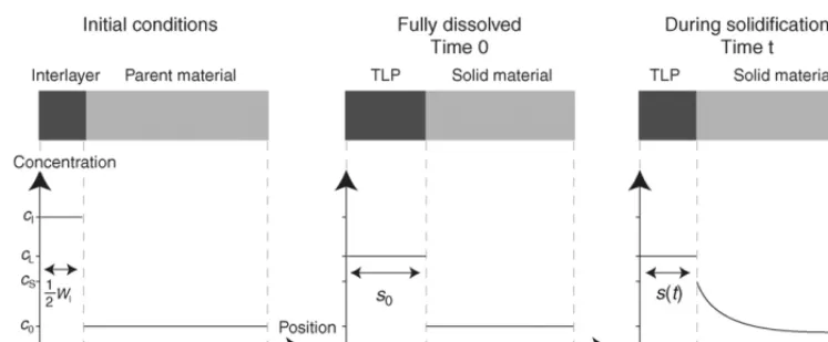
Fig. 1. Schematic representation of the evolving concentration profile. In modelling the process, only the solidification step is considered, with the conditions after dissolution (at timet= 0) being derived from a simple mass balance. Because of the symmetry of the system, only half the joint need be considered.

the present work is to identify values of the two parameters for which these approximations are valid and, consequently, to spec-ify the circumstances under which the corresponding analytical formulae provide an appropriate description of the real physical process. Maps are presented which allow this assessment to be made for real systems. Only isothermal solute transport is con-sidered, so that any phenomena affected by heat flow, such as transient behaviour during heating and cooling, are outside the scope of this paper.

2. Mathematical formulation

2.1. Governing equations and boundary conditions

The physical description of TLP bonding as a diffusion-controlled phase change is well-established [4–7,11–19] and simulations made on this basis have been found to agree reason-ably well with experimental observations[12,13]. Although the mathematical models used previously differ slightly from each other, there is general agreement on the nature of the underlying physical phenomena.

Bonding operations may be understood by breaking the pro-cess down into a sucpro-cession of discrete steps[4,5]. This can be rather confusing, since the stages often occur simultaneously, and the transition between them is inevitably blurred. However, it is certainly true that bonding progresses via two distinct regimes. At short times, rapid solute transport in the liquid means that atomic fluxes in that phase dominate the rate at which dissolu-tion of the parent material occurs. Once the liquid has become homogeneous, solidification takes place at a rate determined by the rate of diffusion within the solid phase. This assumption is supported by numerical simulations[4,6,20].

Since diffusion in the solid is relatively slow, the solidification step generally takes much longer to complete than initial dissolu-tion. In determining the economic viability of any heat treatment, the total duration is of major concern. The time required for solidification is therefore of primary interest when deciding whether any particular system is suitable for TLP bonding. For this reason, the attention of the present work is restricted to a description of the solidification process.

Generally, the pieces to be joined are planar (or have low curvatures). While some concerns have been expressed

[5,12,17–19]as to whether the interface remains planar during solidification if the parent material is polycrystalline, the pro-cess is usually modelled as illustrated schematically inFig. 1. Only half the system need to be considered, due to the inherent symmetry of the bond.

The initial half-thickness of the liquid layer at the onset of solidification (s0) may be determined by a simple solute balance, which assumes that none of the MPD enters the solid during dissolution[15]. It is convenient to introduce a system of co-ordinates in which the origin lies at the centre of the bond-line; the symbolxis used to denote this positional variable, and the position of the inter-phase interface iss(t). The evolving concen-tration profile in the solid region satisfies Fick’s second law[21]. Writingc(x,t) for the atomic concentration, this can be expressed as

∂c(x, t)

∂t =

∂ ∂x

D∂c(x, t) ∂x

, s(t)≤x≤L, t≥0 (1)

whereDdenotes the diffusion coefficient of the MPD in the solid andLcorresponds to the (half-) thickness of the system.

com-pensates for the fact that the molar volume of solid and liquid may be different[24]. The conservation requirement is therefore written in the general case as

−D∂c(x, t)

∂x =(cS−c∗L) ds(t)

dt , x=s(t), t≥0 (2)

in whichc∗Lis the effective liquidus concentration. Estimation ofc∗_Lfor any particular case can be carried out using the balance approach[23].

To complete the mathematical statement of the problem, initial and boundary conditions for the governing differential equations must be specified. In the TLP bonding operations of interest here, the boundary conditions are

c(x, t)=cS, x=s(t), t≥0 (3) ∂c(x, t)

∂x =0, x=L, t≥0 (4)

and the initial conditions are

c(x, t)=c0, s(t)< x≤L, t=0 (5)

s(t)=s0, t=0 (6)

Eqs. (1)–(6) give a complete mathematical description of the process. Several authors [6,11,13,14] have used similar expressions to investigate how different systems are expected to behave. Subject to the auxiliary assumption thatDis a con-stant (independent of concentration), it is possible to write the governing Eqs.(1)–(6) in non-dimensional form. Introducing the following dimensionless variables

τ= Dt s2 0

(time)

ρ=_sx 0

(position)

γ= c−c0 cS−c∗_L

(concentration)

σ= s(t) s0

(interface position)

allows the governing equations to be expressed

∂γ(ρ, τ)

∂τ =

∂2_{γ(ρ, τ)}

∂ρ2 , σ(τ)≤ρ≤P, τ≥0 (7) ∂γ(ρ, τ)

∂ρ = −

dσ(τ)

dτ , ρ=σ(τ), τ ≥0 (8)

subject to

γ(ρ, τ)=Ω, ρ=1, τ≥0 (9)

∂γ(ρ, τ)

∂ρ =0, ρ=P, τ≥0 (10)

γ(ρ, τ)=0, 1< ρ≤P, τ =0 (11)

σ(τ)=1, τ=0 (12)

in which

P = L s0

Ω= cS−c0 cS−c∗L

In this form, it is clear that the process of solidification is a function of only two dimensionless parameters:

• a thermodynamic parameter,Ω, and • a geometric parameter,P.

The diffusivity (D) and the initial thickness of the liquid layer (s0) affect solidification only in a self-similar manner. Doubling the value ofDmerely means that the process will progress twice as quickly. Increasing the width of the liquid layer by a factor of two means that solidification will take four times as long.

The liquidus, solidus and far field concentrations do not them-selves govern the rate of solidification. Rather, it is a ratio of concentration differences that determines this[4,6]. The impor-tance of the ‘saturation parameter’Ωin characterising diffusion-controlled phase changes has also been recognised in other contexts, especially precipitation reactions[1]. For TLP solid-ification,cS>c0andc∗L> cS, which means thatΩ< 0, so that the ‘saturation’ is actually a sub-saturation.

This non-dimensional formulation of the problem indicates that TLP solidification can be characterised solely by the val-ues of the ratios ΩandP, since they are the only parameters that affect the mathematical behaviour of the solution to Eqs.

(7)–(12). The effect of Ω on solidification kinetics has been studied in detail[4,6]. However, the way in whichPaffects the kinetics of the process is not fully known, although it is clear that effects of the ratiosΩandPare strongly coupled. This issue is addressed below.

2.2. Analytical solution

Diffusion-controlled moving boundary (“Stefan”) problems frequently occur in various natural phenomena. As Crank has reported in great detail [22], numerous attempts have been made to solve them, using various techniques. Unfortunately, exact (closed form) solutions are only available for certain, very restricted, cases. In the current context, only one useful solution of Eqs.(7)–(12)is available. In dimensionless terms, it can be written as

γ(ρ, τ)= Ω erfc (κ)erfc

1−ρ √

4τ

(13)

where erfc(γ) denotes the complementary error function ofγ, and the interface motion equation is

s(t)=s0+κ √

4Dt (14)

in which the constantκremains to be determined.

system were infinitely large (L→ ∞), the boundary condition

(4)could be replaced by the equivalent requirement that

c(x, t)=c0, x→ ∞, t≥0 (15)

In this case, Eq.(13)satisfies all of the conditions required of the solution. The analytical solution is therefore applicable only when the system is infinitely large (semi-infinite).

Of greater practical interest than the concentration profile is an expression for the rate at which the interface moves. The ‘solidification rate constant’κ, can be evaluated by differentiat-ing Eq.(14)and substituting this differential into Eq.(2), leading to[12]

√

πκerfc(κ) exp(κ2)=Ω (16)

It has thus been demonstrated that the rate of solidification depends only onΩwhen

P = L s0 → ∞

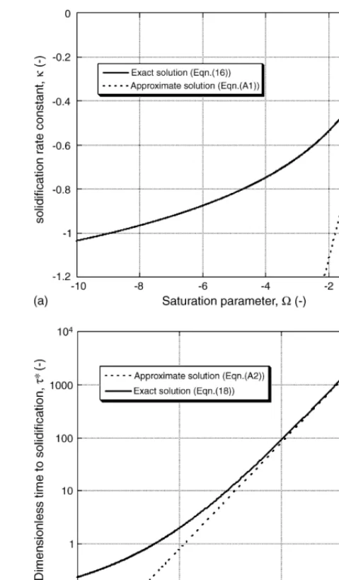
Unfortunately, Eq. (16)constitutes a complex relationship betweenΩandκ. Since it is transcendental in nature, it cannot be inverted algebraically, so it is not possible to express in closed form how the rate of solidification depends on Ω. Instead, it must be solved numerically, to find the appropriate value forκ. The outcome of this operation, carried out using a commercial software package[25], is presented inFig. 2(a).

Large negative saturations are associated with large negative values of κ, which implies a fast-moving interface. It follows that those systems in whichΩhas a large absolute value solid-ify fastest (other things being equal). In view of the physical interpretation which may be placed onΩ(a measure of the driv-ing force available to move the interface relative to the drivdriv-ing force required to move it), this is physically intuitive.

Because costs associated with heat treatments depend criti-cally on their duration, the time to solidification,t*, is important. Using the condition

s(t∗)=0

it is possible to derive[12,14]

t∗= s20

4Dκ2 (17)

or, in non-dimensional terms,

τ∗= 1

4κ2 (18)

Sinceκ is a function ofΩ, the influence of this thermody-namic parameter on the kinetics of solidification is clear. By combining Eqs.(16)and(18), it is possible to determine how the saturation parameter affects the time to solidification, a func-tional dependency illustrated inFig. 2(b). Times to solidification vary over several orders of magnitude, for values of Ω that are typically observed in metallic systems. The thermodynamic characteristics of an alloy system are therefore expected to have a strong influence on its viability for use in TLP bonding.

In order to relate Eq.(17)to parameters directly controllable as process variables, it may be assumed that the inter-layer has

Fig. 2. (a) Dependence of the solidification rate constant,κ, on the sub-saturation parameter,Ω. (b) Dimensionless time to solidification,τ*_{, as a function of} sub-saturation,Ω(for systems in which the solute sink may be considered infinitely large).

an initial widthWIand a homogenous compositioncI. A simple mass balance then requires that the initial thickness of the liquid layer (after completion of dissolution) satisfies

WIc∗I +(2s0−WI)c0=2s0c∗L,

withc∗_I corrected for density differences between the phases. Rearrangement of the terms gives

s0= W I 2

c∗

I −c0 c∗

L−c0

(19)

implying that

t∗= WI2 16Dκ2

_c∗

I −c0 c∗L−c0

2

. (20)

pre-viously been pointed out[14]that these can contain significant errors, although this covered only fixed values of concentra-tionc0, whereasFig. 2(b) reduces the comparison to a single dimensionless plot, illustrating the value of dimensionless rep-resentation in Eqs.(7)–(12). In fact, as is shown inAppendix A, these alternative expressions are accurate only in the limit when Ω→0, as indicated inFig. 2.

2.3. Numerical solutions

For many engineering applications, the thickness of the pieces to be joined is often large (relative to diffusion distances). In such circumstances, the solid region may effectively be con-sidered semi-infinite, and the formulae presented in the previous section may be used to predict the solidification behaviour. In certain applications, however, the ‘infinite sink’ approximation is unlikely to be valid. For example, TLP processing is rou-tinely used in the microelectronics industry to bond very small components [9–11]. Since it is not obvious how the kinetics of solidification might be affected when the solid region is of finite size, it remains unclear as to when the analytical solution presented earlier is appropriate. This question is now addressed. No exact solution is available for the finite case, so numerical approximations must be used if the magnitude of the ‘finite size effect’ is to be assessed. The present authors recently published

[16,20]an algorithm designed to obtain approximate solutions to Eqs.(1)–(6), to any required accuracy. By comparing numer-ical output from that algorithm with predictions generated using the exact solution presented in the previous section, the cir-cumstances under which the ‘infinite sink’ approximation is acceptable can be investigated. (For all of the numerical results presented here, the time-step and space-step of the finite dif-ference solution were chosen to be sufficiently small so that further refinements led to no discernable differences.)Fig. 3

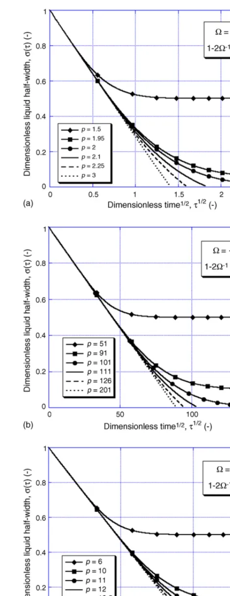
illustrates how the thickness of a liquid region varies as a func-tion of time, in terms of the dimensionless parameters defined earlier (for systems of various sizes and for three different values of the saturation parameter). In every case, the interface displace-ment is predicted to depend on√tat short times, in accordance with Eq. (14). For systems in which the solid sink is of lim-ited extent, however, deviation from this ‘parabolic’ behaviour rapidly occurs, with solidification progressing at a slower rate. Clearly, this is because the presence of a fixed boundary dis-turbs the diffusion profile. As concentration gradients in the solid become less steep than in the infinite case, the rate at which the MPD is transferred from liquid to solid is correspondingly reduced and solidification is slowed.

For systems in whichP has a sufficiently large value (i.e. when the parent material is thick), the evolving diffusion profile is not affected by the presence of the fixed boundary. In these cases, it is appropriate to consider the system as though it were infinite, so that the thickness of the liquid region is predicted to vary with the square root of time until solidification is complete. The values ofκimplied by these numerical results are found to be almost exactly equal to those given by Eq.(16).

The tendency for a fixed boundary to retard solidification is observed in all cases, irrespective of the value of the saturation

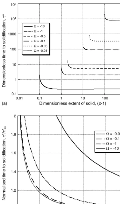
Fig. 4. Time required to completely solidify the liquid, as a function of the size of the solid region, expressed in (a) dimensionless units and (b) normalised units. parameter. However, the actual size of solid material that may be considered ‘sufficiently large’ for edge effects to be neglected depends critically on Ω. To illustrate this effect more easily,

Fig. 4presents data for the dimensionless time required to solid-ify the liquid phase, (τ*) as a function of the dimensionless extent of the solid region (P−1), for various values ofΩ.

From Fig. 4(a), it may be concluded that, for increasingly thick solid pieces (P→ ∞), the dimensionless time to

solidifica-tion tends to a fixed value,τ_∞∗ (which depends on the saturation parameter). This value can be calculated using Eq. (18). For smaller systems, the time to solidification is longer. At some critical size of system,Lcrit (or, equivalently,Pcrit), the time to solidification becomes infinite. This corresponds to a system in which the solid would become totally saturated in solute just at the moment when the liquid is completely consumed. The critical size therefore depends on the liquidus and solidus con-centrations, and can be calculated on the basis of a simple mass balance

c∗Ls0+c0(Lcrit−s0)=cSLcrit

In terms of the dimensionless parameterΩ, this can be expressed as

Pcrit−1= −Ω−1 (21)

Using Eqs.(18)and(21), it is possible to normalise the axes ofFig. 4(a). Associated results are presented inFig. 4(b), which shows that values for the time to solidification which are subject to the infinite matrix approximation contain errors of less than 2% for

P−1 Pcrit−1 >

2 (22)

when|Ω|< 1 (i.e. for saturations common in metallic alloys). According to Eq.(21), this means that the infinite sink approxi-mation is suitable for systems whereP> 1−2Ω−1(if|Ω|< 1). Such a conclusion is supported by the data presented inFig. 3, which confirm that (for systems of this size) the motion of the interface follows a√tdependency, indicating that the effect of the far boundary is insignificant.

2.4. Application to real systems

Subject to the identification of a suitable MPD to use as an inter-layer, any material could theoretically be joined using the TLP bonding technique. In practice, it has been used in only a few alloy systems, probably because it is generally assumed that the diffusivity of the melting point depressant must be high if solidification is to be completed in a reasonable time. (The review of MacDonald and Eagar[4]mentions a lower limit of around 10−12m2s−1, which effectively constitutes a restriction to elements that diffuse interstitially.) However, the preceding analysis demonstrates that the time required to solidify a TLP also depends on factors other than the value ofD—the saturation parameterΩ, for example (seeFig. 2(b)). These other factors should also be taken into account when selecting an MPD inter-layer.

Consider, for instance, inter-layers for use in the bonding of nickel, a candidate for use in high temperature MEMS pack-ages. (Other systems, such as Au/Sn/Au and Ag/Cu/Ag, are of interest for microelectronic applications[11].) Commonly, fast-diffusing interstitial elements, such as boron[5]or phos-phorus[13], are employed as the MPD. However, these elements have a very low solubility, and a relatively high liquidus con-centration, in Ni. Other elements, vanadium, for example, have rather different characteristics, as can be seen from the phase diagrams presented inFig. 5. In order to assess which candi-date material constitutes the most effective inter-layer (the one which would lead to most rapid solidification), it can be assumed that the solid is sufficiently large that the exact analytical solu-tion may be used. An estimate can then be made of the time required to solidify a liquid layer containing one of these ele-ments during a heat treatment at, say, 1200◦C. Zhou and North

[13]previously considered precisely this problem, for the case where the MPD is phosphorous. If the Ni is pure (c0= 0), the liquidus and solidus values they quote correspond to a satura-tion parameter ofΩP=−0.017. They used a diffusivity value of

Fig. 5. Binary phase diagrams[26]between Ni and candidate elements for its TLP bonding: (a) phosphorus and (b) vanadium. the case of vanadium, the saturation parameter is estimated from

the conditions at the eutectic temperature, giving ΩV=−5.3. Standard data[26]are used to calculate the inter-diffusivity of V in Ni, resulting in a value ofDV= 4.6×10−14m2s−1. (In both cases, the difference in molar volume between solid and liquid phases has been neglected.)

Extrusion of liquid from between the faying surfaces is rou-tinely reported during TLP bonding experiments[4]. This being the case, Eq. (19)is unlikely to yield an accurate estimate of the thickness of the liquid layer at the start of solidification. In fact, the amount of liquid present is more likely to be deter-mined by the physical characteristics of the material to be joined (roughness, for example), than by the chemical identity of the inter-layer. On this basis, the thickness of liquid present at the start of solidification when either V or P is used to bond Ni may be assumed to be approximately equal. From Eq.(17), it is therefore possible to write

t∗P t∗

V

=κ2VDV κ2

PDP

Substituting values forκcalculated from a numerical solution to Eq. (16), this ratio is found to be approximately 20. This implies that, during an isothermal heat treatment at 1200◦C, a liquid layer caused by the presence of V solidifies about twenty times faster than one of the same size containing P. The more rapid diffusion of P is thus insufficient to compensate for the effects of its very limited solubility.

In general, since interstitial elements tend to strain the lattice of the parent material, high concentrations of such elements are energetically unfavourable. This limited solubility means that it is difficult to establish steep concentration gradients when the MPD is an interstitial element. Shallow gradients will give rise to small atomic fluxes, even if the (interstitial) MPD has a high diffusivity. On the other hand, it is often possible to accommo-date large concentrations of a substitutional MPD. Large fluxes could then be generated, despite the slower diffusivities. Solidi-fication may still be more rapid, therefore, than in the interstitial case.

These arguments serve to demonstrate that a full understand-ing of the bondunderstand-ing process is needed if the optimal (fastest solidifying) inter-layer materials are to be identified for any par-ticular application. While TLP bonding is a diffusion-controlled process, diffusivity data alone are inadequate for assessing the suitability of potential candidates. Of course, other factors, such as a low eutectic temperature, poor wettability, a propensity to form other phases, a tendency to cause embrittlement, etc., may place further constraints on the choice of inter-layer. Neverthe-less, the example provided by this cursory assessment of two candidate MPDs for joining Ni clearly illustrates the point that a complete understanding of the phenomenon is required in order to select the best inter-layer.

3. Conclusions

A study has been made of the mathematical characteristics of a well-established model for solidification of TLP bonds in binary alloy systems. The main conclusions may be summarised as follows:

(a) The rate of solidification may be characterised by two dimen-sionless parameters: one (Ω) relates to the concentration gradients and thermodynamic characteristics of the system and the other (P) relates to geometrical factors.

(b) Physical parameters, such as the diffusivity and the maxi-mum extent of the liquid region, are found to affect predic-tions only in a self-similar manner.

(c) Exact analytical expressions for the time required for com-plete solidification are available for the case where the solid is of infinite extent.

(d) For conditions typically encountered during TLP bonding, the exact expressions are accurate to within 2% for finite systems whenP> 1−2Ω−1(if|Ω|< 1).

(e) Decreasing the extent of the solid region will increase the time required for complete solidification.

exam-ple of this, elements forming interstitial solutes in the parent material may lead to slower bonding than others forming substitutional solutes, despite their faster diffusion rates.

Acknowledgements

This work has been supported via a Domestic Research Scholarship from the University of Cambridge and an EPSRC Platform Grant.

Appendix A

The derivation of Eq.(17)as a means of estimatingt*uses the exact solution to the system of differential equations expressed in Eqs. (1)–(6). Some authors [7,15]have presented different formulae. These were derived using expressions that do not con-stitute an exact solution to the governing equations and, as such, may be considered erroneous. As Zhou has pointed out[14], these solutions use an expression for the evolving concentration profile which does not take account of the motion of the inter-phase boundary. Rather, the concentration profile is described as though the interface were stationary. On the basis of this expres-sion, interfacial fluxes are calculated and the rate of interface motion is estimated. The resulting expressions therefore consti-tute what may be termed ‘quasi-static’ solutions.

Numerical calculations have shown [14]that the resulting predictions may contain significant errors (when compared with the exact solution). In fact, it is possible to reconcile the exact and quasi-static solution, showing that the latter is actually a particular case of the former with validity restricted to the case whereΩ→0. Since this corresponds to the case where the inter-face moves very slowly, the ‘quasi-static’ assumption implicit in its derivation may equally be understood on a purely physical basis.

More rigorously, the expansions

erfc(κ)=1−√2 π

∞

i=0

(−1)iκ2i+1 (2i+1)×i!

and

exp(κ2)=

∞

i=0 κ2_i

i!

mean that Eq.(19)can alternatively be expressed as

Ω=√π

κ−√2 πκ

2_+κ3_{+ · · ·}

Therefore, for slowly moving interfaces (smallκ)

κ≈ √Ω

π (A.1)

Substituting expression(A.1)into Eq.(18)gives τ∗= π

4Ω2 (A.2)

Estimating the value ofs0using Eq.(19), the time to solidi-fication can be calculated as

t∗_≈ π

16D

WIc

∗

I −c0 c∗

L−c0 cS−c∗_L cS−c0

2 ≈ π

16D

WI c

∗

I cS−c0

2 ,

(A.3)

since small values ofκcorrespond to smallΩ(which implies thatcI≥cLcS>c0).

Eq.(A.3)is exactly the result proposed by Tuah-Poku et al.

[15]and Liu et al.[7](whose investigations were restricted to the particular case wherec0= 0 and liquid and solid densities are equal). Given that the validity of this approximation is limited to applications in whichcI≥cLcS>c0, and given that the exact solution is not very much more complicated, it would be preferable to use Eq.(17)to estimatet*, withκdetermined either graphically (fromFig. 2) or numerically (from Eq.(16)).

References

[1] D.A. Porter, K.E. Easterling, Phase Transformations in Metals and Alloys, Stanley Thornes, Cheltenham, 1992.

[2] R.A. Tanzilli, R.W. Heckel, Metall. Trans. A 2 (1971) 1779–1784. [3] R.W. Heckel, A.J. Hickl, R.J. Zaehring, R.A. Tanzilli, Metall. Trans. 3

(1972) 2565–2569.

[4] W.D. MacDonald, T.W. Eagar, Ann. Rev. Mater. Sci. 22 (1992) 23–46. [5] W.F. Gale, D.A. Butts, Sci. Technol. Weld. Joining 9 (2004) 283–300. [6] Y. Zhou, W.F. Gale, T.H. North, Int. Mater. Rev. 40 (1995) 181–196. [7] S. Liu, D.L. Olson, G.P. Martin, G.R. Edwards, Weld. J. 70 (1991)

S207–S215.

[8] J.D. Sugar, J.T. McKeown, T. Akashi, S.M. Hong, K. Nakashima, A.M. Glaeser, J. Eur. Ceram. Soc. 26 (2006) 363–372.

[9] W.C. Welch, J. Chae, K. Najafi, IEEE Trans. Adv. Packaging 28 (2005) 643–649.

[10] E. Lugscheider, K. Bobzin, M. Maes, S. Ferrara, A. Erdle, Surf. Coat. Technol. 200 (2005) 444–447.

[11] S.R. Cain, J.R. Wilcox, R. Venkatraman, Acta Mater. 45 (1997) 701– 707.

[12] W.D. MacDonald, T.W. Eagar, Metall. Mater. Trans. A 29 (1998) 315– 325.

[13] Y.H. Zhou, T.H. North, Z. MetaIlkd. 85 (1994) 775–780. [14] Y. Zhou, J. Mater. Sci. Lett. 20 (2001) 841–844.

[15] I. Tuah-Poku, M. Dollar, T.B. Massalski, Metall. Trans. A 19 (1988) 675–686.

[16] T.C. Illingworth, I.O. Golosnoy, J. Comput. Phys. 209 (2005) 207–225. [17] K. Ikeuchi, Y. Zhou, H. Kokawa, T.H. North, Metall. Trans. A 23 (1992)

2905–2915.

[18] H. Kokawa, C.H. Lee, T.H. North, Metall. Trans. A 22 (1991) 1627–1631. [19] K. Saida, Y. Zhou, T.H. North, J. Mater. Sci. 28 (1993) 6427–6432. [20] T.C. Illingworth, I.O. Golosnoy, V. Gergely, T.W. Clyne, J. Mater. Sci. 40

(2005) 2505–2511.

[21] J. Crank, The Mathematics of Diffusion, Clarendon Press, Oxford, 1976.

[22] J. Crank, Free and Moving Boundary Problems, Clarendon Press, Oxford, UK, 1984.

[23] M. Rappaz, M. Bellet, M. Deville, Numerical Modeling in Materials Sci-ence and Engineering, Springer-Verlag, Berlin, 2003.

[24] A.G. Guy, R.T. DeHoff, C.B. Smith, Trans. ASM 61 (1968) 314–320. [25] S. Wolfram, The Mathematica Book, Wolfram Media, Cambridge

Univer-sity Press, 1996, p. 895.