Joint Maximum Likelihood Channel Estimation and
Data Detection for MIMO Systems
Mohammed Abuthinien, Sheng Chen, Andreas Wolfgang and Lajos Hanzo
School of Electronics and Computer ScienceUniversity of Southampton Southampton SO17 1BJ, UK
E-mails:{msaa05r,sqc,aw03r,lh}@ecs.soton.ac.uk
Abstract— Blind and semiblind adaptive schemes are proposed for joint maximum likelihood (ML) channel estimation and data detection for multiple-input multiple-output (MIMO) systems. The joint ML optimisation over channel and data is decom-posed into an iterative two-level optimisation loop. An efficient global optimisation search algorithm called the repeated weighted boosting search is employed at the upper level to identify the unknown MIMO channel model while an enhanced ML sphere detector called the optimised hierarchy reduced search algorithm aided ML detector is used at the lower level to perform the ML detection of the transmitted data. A simulation example is included to demonstrate the effectiveness of these two schemes.
I. INTRODUCTION
Multiple-input multiple-output (MIMO) technology has emerged recently as one of the most significant technologies in modern communication. By using MIMO technology an increase in the system capacity and/or an improvement in the quality of service can be achieved [1]-[4]. The key to fully utilise the MIMO capacity relies heavily on the requirement of accurate channel estimation. MIMO channel estimation methods can be classified into three categories: training-based methods, blind methods and semi-blind methods. For pure training-based schemes, a long training is necessary in order to obtain a reliable MIMO channel estimate which reduces the system bandwidth efficiency considerably. Blind methods which do not require any training symbols achieve high system throughput at the expense of high computational complexity. Semi-blind schemes on the other hand require less compu-tational complexity than blind methods and fewer training symbols than training-based methods, making them attractive for practical implementation.
Many blind channel identification techniques can be found in the literature, and a good overview is given in [5]. The blind channel identification methods can be classified into higher-order statistics based techniques [6]-[8] and second-order statistics based techniques [9],[10]. Joint blind channel estimation and data estimation detection has been proposed based on the iterative least squares with projection [11]-[13]. This scheme estimate the channel and data iteratively but the convergence of the scheme depends on the initialisation of the channel model. In the context of MIMO systems, semi-blind schemes have been developed [14]-[17]. These schemes use a few training symbols to provide the initial MIMO channel estimation and exchange the information between the channel
estimator and the data detector iteratively. In this paper we propose blind and semi-blind joint maximum likelihood (ML) channel and data estimation schemes for MIMO channels. Our work extends the approach developed in [18]-[21], in which the joint ML optimisation process for channel and data estimation is decomposed into two levels. At the upper level a global optimisation algorithm searches for an optimal channel estimate, while at the lower level an ML data detector decodes the transmitted data. The joint ML channel estimation and data detection is achieved by exchanging the information between the channel estimator and the data detector iteratively. More specifically, we use the optimised hierarchy reduced search algorithm aided ML (OHRSA-aided ML) detector [22],[23], which is an advanced extension of the complex sphere decoder [24], as the data detector and the repeated weighted boosting search (RWBS) algorithm [20], which is a simple yet efficient global optimisation search routine, as the MIMO channel estimator. Our proposed blind MIMO scheme is formed by it-erating between the RWBS channel estimator and the OHRSA-aided ML data detector. In blind joint MIMO channel and data estimation, permutation ambiguity corresponding to reordering the detected transmitted data and estimation channel matrix columns cannot be resolved by the blind scheme itself. One way of solving this permutation ambiguity is to employ a few pilot training symbols. Further exploiting these training symbols to initialise the search in the RWBS channel estimator yields our proposed semi-blind scheme.
Throughout the paper we adopt the following notational con-ventions. Boldface capital and small letters stand for matrices and vectors, respectively. IK denotes the K ×K identity matrix, and()T and()H are the transpose and hermitian op-erators, respectively.| |denotes the magnitude of a complex value, while 2 is the norm operator. For arbitrary matrix
A, its(i, j)entry is written asA(i, j) =ai,j.
II. SYSTEMMODEL
We consider the MIMO system withM transmit antennas and P receive antennas. It is assumed that the channel coherence bandwidth is larger than the transmitted signal bandwidth so that the channel can be considered as narrowband or flat fading. Furthermore, the channel is assumed to be stationary during the communication process of N symbols. The baud rate sampled received signal at receive antenna p can be
written as
yp(k) = M
m=1
hp,msm(k) +np(k), (1)
where k is the symbol index, hp,m is the complex-valued narrowband channel coefficient connecting transmit antenna m to receive antenna p,sm(k)is thekth transmitted symbol from transmit antennamthat takes value from the binary phase shift keying (BPSK) symbol set {−1,+1}, and np(k) is the complex-valued additive white Gaussian noise (AWGN) with
E[|np(k)|2] = 2σ2
n.
The overall system can be described by the well-known MIMO channel equation as
y(k) =H s(k) +n(k), (2)
where n(k) = [n1(k) n2(k)· · ·nP(k)]T, s(k) = [s1(k)s2(k)· · ·sM(k)]T is the transmitted symbols vector,
y(k) = [y1(k)y2(k)· · ·yP(k)]T is the received signal vector
andH is the P×M channel matrix withH(p, m) =hp,m.
III. THEPROPOSEDBLINDSCHEME
The proposed blind scheme depends only on the observation vectory(k)over a relatively short lengthNof the transmitted data sequence to perform the joint data and channel estimation. Let us define the P ×N matrix of received data and the corresponding M ×N matrix of transmitted data as
Y= [y(1) y(2)· · ·y(N)] (3)
and
S= [s(1) s(2)· · ·s(N)], (4)
respectively. Then the probability density function of the received signal matrix Y conditioned on the MIMO channel matrixH and the transmitted data matrixScan be written as
p(Y|H,S) = 1
(2πσ2
n)NP e−2σ12n
N
k=1y(k)−H s(k)2. (5)
The ML estimation of the transmitted symbols S and the MIMO channel matrix H can be obtained by maximising p(Y|H,S)over S andH jointly. Equivalently, the joint ML estimation can be obtained by minimsing the following cost function
JML(ˇS,Hˇ) = 1 P×N
N
k=1
y(k)−Hˇ ˇs(k)2, (6)
namely, the joint ML channel and data estimation is obtained as
(ˆS,Hˆ) = arg
min
ˇ
S,Hˇ JML(ˇS, ˇ H)
. (7)
From equation (7) it can be seen that the search for the optimal joint ML solution is over the discrete space of the transmitted symbols and the continuous space of the MIMO channel matrix jointly. This search is computationally prohibitive. The complexity of this optimisation process can be reduced to a tractable level if it is decomposed using an iterative loop first
over all the possible data symbols and then over all the possible channel matrices as
(ˆS,Hˆ) = arg
min
ˇ
H
min
ˇ
S JML(ˇS, ˇ H)
. (8)
At the inner or lower-level optimisation we use the OHRSA-aided ML detector to find the ML data estimate for the given channel. The OHRSA-aided ML detector was proposed in [22],[23] where the detailed implementation of this detector can be found. In order to guarantee a joint ML estimate, the search algorithm used at the outer or upper-level optimisation should be capable of finding a global optimal channel estimate efficiently, and we employ the RWBS algorithm to perform the upper-level optimisation. The detailed implementation of this search algorithm can be found in [20].
The proposed blind scheme for MIMO ML channel estimation and data detection is summarised as follows.
Outer-level Optimisation: The RWBS algorithm searches the MIMO channel parameter space to find a global optimal estimateHˆ by minimising the mean square error (MSE)
JMSE( ˇH) =JML(ˆS( ˇH),Hˇ), (9)
where Sˆ( ˇH)denotes the ML estimate of the transmitted data for the given channel Hˇ.
Inner-level Optimisation: Given the MIMO channel matrixHˇ the OHRSA-aided ML detector finds the ML estimate of the transmitted data and feeds back the corresponding ML metric JMSE( ˇH)to the upper level.
The channel gain at each receive antanne can always be normalised to unityMm=1|hp,m|2= 1. This is realistic as the channel energy at each receive antennaσ2sMm=1|hp,m|2 can always be estimated, where σ2s is the known symbol energy. With this normalisation, the RWBS algorithm can set the search range for the real and imaginary parts of each channel coefficient to(−1, 1).
Scaling and permutation ambiguity. Blind joint data and channel estimation for MIMO channels has an inherent permu-tation and scaling ambiguity problem. Scaling ambiguity refers to the fact that the detected data and the estimated channel matrix columns can only be resolved with a complex-valued factor. This scaling factor depends on the modulation scheme, and in the case of BPSK modulation, it takes the values from {+1,−1}. In the permutation ambiguity, the detected data and the estimated channel matrix columns are reordered. The reason for this is clear from the cost function defined in equation (6). This cost function is invariant with respect to a reordering and scaling of the channel matrix and the data matrix. More specifically, let a joint ML estimation of the transmitted data and MIMO channel beSˆ andHˆ. Next define
ˆ
H∗ andSˆ∗ as [25]: ˆ
H∗= ˆH T and Sˆ∗=THSˆ, (10)
whereTis the unitaryM×M permutation and scaling matrix with only one nonzero element in each column and row. Then
The nonzero entries of T depend on the modulation scheme used, and in the BPSK case they take the values from {+1,−1}.
The scaling ambiguity can be resolved easily by using a differ-ential encoding of data. The permutation ambiguity however cannot be resolved easily. In practice this ambiguity is resolved by other means. For example, in CDMA based systems, unique user signiture sequences can be exploited at the receiver to distinguish each user correctly. The scaling and permutation ambiguity can be solved simultaneously if a few pilot training symbols are available. By sending a short training sequence from each transmit antenna, the receiver can identify the correct unitary matrix Tfrom all the possible realizations of this matrix based on the following ML criterion
T= arg min
ˇ
T
Yt−Hˆ T Sˇ t
2
, (12)
where Yt and St are the received and transmitted data matrices, havingNT columns and similar to the ones defined in equations (3) and (4), respectively, during the training, and NT is the length of training.
Computational complexity. Let COHRSA−ML(N) denote the complexity of the OHRSA-aided ML algorithm to decode theN-sample data matrixSandNOHRSA−MLbe the number of calls for the OHRSA-aided ML algorithm required by the RWBS algorithm to converge. Then the complexity of the proposed blind method is given by
C=COHRSA−ML(N)×NOHRSA−ML. (13) The complexity of the OHRSA-aided ML detector is difficult to find precisely as it depends on the signal-to-noise ratio (SNR), but this complexity is increasing with the data length N. The RWBS algorithm is a simple yet efficient global search algorithm. In [21], both the genetic algorithm (GA) and the RWBS algorithm were used to find the ML channel and data estimation for single-input multiple-output systems, and it was seen that the RWBS algorithm achieved slightly better accuracy at the same convergence speed as the GA. The RWBS algorithm has additional advantages of requiring minimum programming effort and having fewer algorithmic parameters to tune. SinceCOHRSA−ML(N)is increasing with N, it is critical in terms of complexity that the blind scheme can work with as short of the data length as possible. We will demonstrate that our proposed blind method can achieve a joint ML solution with a very short data lengthN through simulation.
IV. THEPROPOSEDSEMI-BLINDSCHEME
As discussed in the previous section, a blind scheme suffers from scaling and permutation ambiguity. One way of resolving
TABLE I
THESIMULATEDMIMO SYSTEM
Tx antenna 1 Tx antenna 2 Tx antenna 3 Rx antenna 1 -0.0314 + 0.0719i 0.3101 + 0.7030i 0.0188 + 0.6350i Rx antenna 2 0.3864 + 0.0120i -0.4124 - 0.3786i 0.5770 - 0.4521i Rx antenna 3 -0.5177 - 0.1239i -0.2124 + 0.2281i 0.0747 + 0.7835i
1000 2000 3000 4000 5000 6000 7000
10−3 10−2 10−1 100
No. of OHRSA−ML evaluations
Mean square error (MSE)
SNR = 5 dB
SNR = 10 dB
SNR = 20 dB
[image:3.595.320.541.56.227.2]SNR = 30 dB
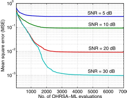
Fig. 1. Mean square error against the number of OHRSA-ML evaluations averaged over 20 different runs for a range of SNR values using the proposed blind ML channel and data estimation scheme, whereN= 50.
1000 2000 3000 4000 5000 6000 7000
10−2 10−1
No. of OHRSA−ML evaluations
Mean channel error (MCE)
SNR = 5 dB
SNR = 10 dB
SNR = 20 dB
[image:3.595.320.543.272.440.2]SNR = 30 dB
Fig. 2. Mean channel error against the number of OHRSA-ML evaluations averaged over 20 different runs for a range of SNR values using the proposed blind ML channel and data estimation scheme, whereN= 50.
this ambiguity is to employ a few pilot training symbols. If we adopt this pilot training approach to resolve the ambiguity of joint ML estimate, we can further exploit this training to provide an initial channel estimate. This naturally leads to a semi-blind scheme, which also reduces the computational complexity considerably, in comparison with the pure blind technique. The proposed semi-blind method follows exactly the same methodology of the blind scheme explained in section III, except that it uses a few pilot training symbols to initialise the RWBS algorithm.
The least squares channel estimation (LSCE) technique is used to find the initial estimate for the channel. The estimated LSCE channel matrix is given by
ˇ
HLSCE =YtSHt
channel estimator are randomly chosen for the blind scheme while for the semi-blind scheme the LSCE HˇLSCE is used as one of the members of the initial channel population. The proposed semi-blind method requires less computational complexity than the blind one and the number of training symbols NT required is very small, as will be demonstrated in the simulation example.
V. SIMULATIONEXAMPLE
The simulated MIMO system consisted of M = 3 transmit antennas and P = 3 receive antennas. Table I shows this simulated3×3MIMO channel matrix. The modulation scheme was BPSK and the length of data sequences wasN = 50. The simulation was carried out using both the proposed blind and semi-blind methods. For the semi-blind scheme, the number of training symbols was NT = 4. In practice the value of the likelihood metric JMSE( ˇH) is all what the upper-level RWBS optimiser can have, and the convergence of the scheme can only be observed through this MSE. However, in the simulation the performance can also be assessed by means of the mean channel error (MCE), which we define as
MCE= 1 M×P
M
m=1
P
p=1
hp,m−Hˆ∗(p, m). (15)
Figs. 1 and 2 show the evolutions of the MSE and MCE averaged over 20 different runs for a range of different SNR values, respectively, obtained by the proposed blind scheme. From Fig. 1 it can be seen that the MSE converged to the noise floor, and at SNR= 20dB the scheme required approximately 2000 OHRSA-ML evaluations to converge. Note that the data length N = 50 was very small and each OHRSA-ML evaluation was performed very fast. The accuracy of the blind scheme can be seen from Fig. 2, where we can see that the proposed blind scheme achieved a high accuracy in estimating the MIMO channel matrix. This accuracy can be seen also from Fig. 3 which shows the bit error rates (BERs) calculated by the ML detectors using the estimated channel matrix obtained by the proposed blind method and the perfect
2 4 6 8 10 12
10−5 10−4 10−3 10−2 10−1
SNR (dB)
BER
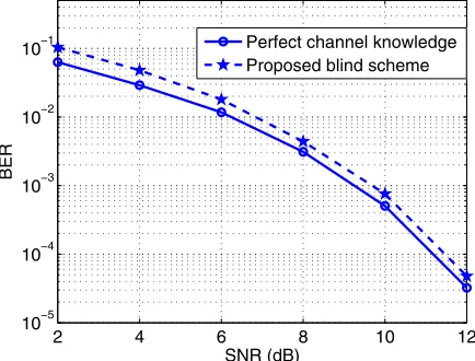
[image:4.595.322.543.120.288.2]Perfect channel knowledge Proposed blind scheme
Fig. 3. Bit error rate comparison for the proposed blind scheme and the perfect channel. The length of data samples for blind scheme wasN= 50.
channel, respectively. For the proposed blind scheme, the BER was averaged over 20 different runs. From Fig. 3, we can see that the proposed blind scheme only induces less than half dB degradation in SNR, compared with the perfect channel case.
200 400 600 800 1000 1200
10−3 10−2 10−1
No. of OHRSA−ML evaluations
Mean square error (MSE)
SNR = 5 dB
SNR = 10 dB
SNR = 20 dB
[image:4.595.320.543.342.511.2]SNR = 30 dB
Fig. 4. Mean square error against the number of OHRSA-ML evaluations averaged over 20 different runs for a range of SNR values using the proposed semi-blind ML channel and data estimation scheme, where N = 50and NT= 4.
200 400 600 800 1000 1200
10−2 10−1
No. of OHRSA−ML evaluations
Mean channel error (MCE)
SNR = 5 dB
SNR = 10 dB
SNR = 20 dB
SNR = 30 dB
Fig. 5. Mean channel error against the number of OHRSA-ML evaluations averaged over 20 different runs for a range of SNR values using the proposed semi-blind ML channel and data estimation scheme, where N = 50and NT= 4.
[image:4.595.59.276.541.706.2]scheme. It can be seen from Fig. 4 that the proposed semi-blind method required approximately 300 OHRSA-ML evaluations to converge, and each OHRSA-ML run is only with respect to a data length of N = 50. This should be compared with the semi-blind MIMO estimation scheme of [17], which requires a data length of N= 200 to work properly.
2 4 6 8 10 12
10−5 10−4 10−3 10−2 10−1 100
SNR (dB)
BER
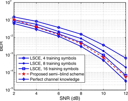
[image:5.595.62.276.140.310.2]LSCE, 4 training symbols LSCE, 8 training symbols LSCE, 16 training symbols Proposed semi−blind scheme Perfect channel knowledge
Fig. 6. Bit error rate comparison for the proposed semi-blind scheme, the perfect channel and the case of the LSCE training based technique with various training lengths. For the semi-blind method,N= 50andNT= 4.
VI. CONCLUSIONS
A blind joint ML scheme for MIMO channel estimation and data detection has been proposed by iterating between the RWBS channel estimator and the OHRSA-aided ML detector. Simulation study has shown that the proposed blind scheme requires a very short data length to achieve excellent accuracy, at the cost of relatively high computational complexity. Like any pure blind method, the proposed blind scheme can only find the joint ML solution up to some permutation and scaling ambiguity. By using a very few pilot training symbols to resolve this ambiguity and to initialise the RWBS channel estimator, a semi-blind scheme has been proposed. It has been shown that this semi-blind scheme significantly reduces the computational complexity and has a slightly better perfor-mance, in comparison with the blind scheme.
ACKNOWLEDGEMENTS
The financial support of the EU under the auspices of the Phoenix and Newcom projects is gratefully acknowledged.
REFERENCES
[1] G.J. Foschini and M.J. Gans, “On limits of wireless communications in a fading environment when using multiple antennas, ”Wireless Personal
Communications, vol.6, no.3, pp.311–335, 1998.
[2] I.E. Telatar, “Capacity of multi-antenna Gaussian channels,”European
Trans. Telecommunications, vol.10, no.6, pp.585–595, 1999.
[3] T.L. Marzetta and B.M. Hochwald, “Capacity of a mobile multiple-antenna communication link in Rayleigh flat fading,” IEEE Trans.
Information Theory, vol.45, no.1, pp.139–157, 1999.
[4] A. J. Paulraj, D.A. Gore, R.U. Nabar and H. B¨olcskei, “An overview of MIMO communications – A key to gigabit wireless,”Proc. IEEE, vol.92, no.2, pp.198–218, 2004.
[5] L. Tong and S. Perreau, “Multichannel blind identification: From sub-space to maximum likelihood methods,” Proc. IEEE, vol.86, no.10, pp.1951–1968, 1998.
[6] J.F. Cardoso, “Source separation using higher ordered moments,” in
Proc. ICASSP-1989, 1989, vol.4, pp.2109–2112.
[7] P. Comon, “Independent component analysis: A new concept?”Signal
Processing, vol.36, no.3, pp.287–314, 1994.
[8] C.-Y. Chi, C.-Y. Chen, C.-H. Chen and C.-C. Feng, “Batch processing algorithms for blind equalization using higher-order statistics,” IEEE
Signal Processing Magazine, vol.20, no.1, pp.25–49, 2003.
[9] C-Q. Chang, S.F. Yau, P. Kwok, F.K. Lam and F.H.Y. Chan, “Sequential approach to blind source separation using second order statistics,” in
Proc. 1st Int. Conf. Information, Communication, ans Signal Processing,
Sept. 9-12, 1997, vol.3, pp.1608–1612.
[10] K. Abed-Meraim, Y. Xiang, J.H. Manron and Y-B. Hua, “A new ap-proach to blind separation of cyclostationary sources,” inProc. 2nd IEEE Workshop Signal Processing Advances in Wireless Communications (Annapolis, MD, USA), May 9-12, 1999, pp.114–117.
[11] S. Talwar, M. Viberg and A. Paulraj, “Blind separation of synchronous co-channel digital signals using an antenna array – Part I: Algorithms,”
IEEE Trans. Signal Processing, vol.44, no.5, pp.1184–1197, 1996.
[12] A. Ranheim, “A decoupled approach to adaptive signal separation using an antenna array,” IEEE Trans. Vehicular Technology, vol.48, no.3, pp.676–682, 1999.
[13] A. Dogandzic and A. Nehorai, “Generalized multivariate analysis of variance - A unified framework for signal processing in correlated noise,”
IEEE Signal Processing Magazine, vol.20, no.5, pp.39–54, 2003.
[14] A. Medles and D.T.M. Slock, “Semiblind channel estimation for MIMO spatial multiplexing systems,” in Proc. VTC2001-Fall, 2001, vol.2, pp.1240–1244.
[15] C. Cozzo and B.L. Hughes, “Joint channel estimation and data detection in space-time communications,”IEEE Trans. Communications, vol.51, no.8, pp.1266–1270, 2003.
[16] S. Buzzi, M. Lops and S. Sardellitti, “Performance of iterative data de-tection and channel estimation for single-antenna and multiple-antennas wireless communications,”IEEE Trans. Vehicular Technology, vol.53, no.4, pp.1085–1104, 2004.
[17] T. Wo, P.A. Hoeher, A. Scherb and K.D. Kammeyer, “Performance anal-ysis of maximum-likelihood semiblind estimation of MIMO channels,”
in Proc. VTC2006-Spring(Melbourne, Australia), May 7-10, 2006, 5
pages.
[18] S. Chen and Y. Wu, “Maximum likelihood joint channel and data estimation using genetic algorithms,” IEEE Trans. Signal Processing, vol.46, no.5, pp.1469–1473, 1998.
[19] S. Chen and B.L. Luk, “Adaptive simulated annealing for optimization in signal processing applications,”Signal Processing, vol.79, no.1, pp.117– 128, 1999.
[20] S. Chen, X.X. Wang and C.J. Harris, “Experiments with repeating weighted boosting search for optimization in signal processing appli-cations,” IEEE Trans. System, Man and Cybernetics, Part B, vol.35, no.4, pp.682-693, 2005.
[21] S. Chen, X.C. Yang and L. Hanzo, “Blind joint maximum likelihood channel estimation and data detection for single-input multiple-output systems,” in Proc. 6th IEE Int. Conf. 3G & Beyond(London, UK), Nov.7-9, 2005, 5 pages.
[22] J. Akhtman and L. Hanzo, “Reduced-complexity maximum likelihood detection in multiple-antenna-aided multicarrier system,” in Proc. 5th
Int. Workshop Multi-Carrier Spread-Spectrum(Oberpfaffenhofen,
Ger-many), Sept. 14-16, 2005, pp.21–28.
[23] J. Akhtman and L. Hanzo, “Maximum-likelihood enhanced sphere decoding of MIMO-OFDM,” in L. Hanzo and T. Keller, OFDM and
MC-CDMA: A Primer, Chichester, UK: John Wiley, 2006, pp.253–301.
[24] D. Pham, K. Pattipati, P.K. Willet and J. Luo, “An improved complex sphere decoder for V-BLAST systems,”IEEE Signal Processing Letters, Vol.11, no.9, pp.748–751, 2004.
[25] L. Tang, R. Lui, V. Soon and Y. Huang, “Indeterminacy and identifia-bility of blind identification,”IEEE Trans. Circuits and Systems, vol.38, no.5, pp.499–509, 1991.
[26] G. Leus and A. van der Veen, “Optimal training for ML and LMMSE channel estimation in MIMO systems,” inProc. IEEE/SP 13th Workshop