Continuation Value Methods for Sequential Decisions: A General Theory

(1)

Continuation Value Methods for

Sequential Decisions:

A General Theory

Qingyin Ma

January 2018

A thesis submitted for the degree of

Doctor of Philosophy of

The Australian National University

c

Copyright by Qingyin Ma 2018

(2)

Declaration

Except where otherwise acknowledged, I certify that this thesis is my original work. The thesis is within the 100, 000 word limit set by the Australian National University.

(3)

(4)

Acknowledgement

First, I would like to express my deepest gratitude to my chair supervisor, Prof. John Stachurski, who continuously encouraged me to reach for a high standard of research and offered me tremendous help and support all the time. Always with patience and great enthusiasm, John guided me along the way in my train-ing of technical skills, and taught me how to find important research questions and come up with general ideas that contribute to frontier research. In doing that, he could always transform very complicated ideas into simple and intu-itive principles, which enhanced my understanding, and helped me solve a lot of challenging problems that I had considered to be out of my reach. Moreover, John motivated me to pursue this project, contributed directly to each chapter of this thesis and provided me with invaluable advice. Without his support, I would not have been able to complete this thesis. I cannot thank him enough.

I would also like to thank my panel supervisors, Prof. Joshua Chan and Dr. Chung Tran, for their insightful comments and criticisms, especially during my seminars and workshops, which incented me to think of my research from vari-ous other perspectives. Other than that, they were always considerate and willing to help when I met difficulties. Their kindness is very much appreciated.

My sincere gratitude also goes to Prof. Boyan Jovanovic, Prof. Takashi Kamihi-gashi and Prof. Hiroyuki Ozaki. Their insightful and constructive suggestions directly improved the quality of this thesis and other related research projects. I would like to give special thanks to Prof. Takashi Kamihigashi and Dr. Daisuke Oyama, for kindly helping me organize seminars and workshops during my re-search visits at Rere-search Institute for Economics and Business Administration, Kobe University, and Faculty of Economics, the University of Tokyo, respectively. Completing a PhD is a challenging journey, yet in my case this journey has been wonderful and enjoyable, thanks to my family and friends. I am very grateful to my parents and sister for their patience and understanding, and for supporting me spiritually on my PhD study. For their feedbacks, cooperation and

(5)

v

ship, I owe a debt of gratitude to my PhD fellows: Azadeh Abbasi-Shavazi, Jamie Cross, Jenny Chang, Minhee Chae, Chenghan Hou, Haidi Hong, Jim Hancock, Syed Hasan, Sehrish Hussein, Bogdan Klishchuk, Anpeng Li, Dan Liu, Weifeng Larry Liu, Arm Nakornthab, Minh Ngoc Nguyen, Michinao Okachi, Aubrey Poon, Christopher Perks, Guanlong Ren, Jie Shen, Luis Uzeda-Garcia, Wenjie Wei, Yanan Wu, Sen Xue, Jilu Zhang, Junnan Zhang, Nabeeh Zakariyya, and Yu-rui Zhang. Special thanks go to Weifeng Larry Liu, for working closely with me on tough research materials for years. His support and patience are greatly ap-preciated.

(6)

Abstract

After the introductory chapter, this thesis comprises four main chapters before concluding in chapter 6. The thesis undertakes a systematic analysis of the con-tinuation value based method for sequential decision problems originally due to

Jovanovic (1982). Although recently this technique is widely employed in a va-riety of economic applications, its theoretical connections to the traditional value function based method, relative efficiency, and optimality/analytical properties have hitherto received no general investigation. The thesis fills this gap.

On the one hand, the thesis shows that the operator employed by this method (referred to below as the Jovanovic operator) is semiconjugate to the traditional Bellman operator and has essentially equivalent dynamic properties. In particu-lar, under general assumptions, any fixed point of one of the operators is a direct translation of a fixed point of the other. Iterative sequences generated by the operators are also simple translations. After adding topological structure to the generic setting, the thesis shows that the Bellman and Jovanovic operators are both contraction mappings under identical assumptions, and that convergence to the respective fixed points occurs at the same rate.

To ensure sufficient generality for economic applications, the optimality and sym-metry analysis has been embedded separately in (a) spaces of potentially un-bounded functions endowed with generic weighted supremum norm distances, and (b) spaces of integrable functions with divergence measured by Lp norms. Unbounded rewards are allowed provided that they do not cause continuation values to diverge. Moreover, the theory mentioned above is established for im-portant classes of sequential decision problems, including:

• standard optimal stopping problems (chapter2),

• repeated optimal stopping problems (chapter3), and

(7)

vii

On the other hand, despite these similarities, the thesis shows that there do re-main important differences between the continuation value based method and the traditional value function based method in terms of efficiency and analytical convenience.

One of these differences concerns the dimensionality of the effective state spaces associated with the Bellman and Jovanovic operators. First, aside from a class of problems for which the continuation dynamics are trivial, the effective state space of the continuation value function is never larger than that of the value function. Second, for a broad class of sequential problems, the effective state space of the continuation value function is strictly lower dimensional than that of the value function. Another key difference is that continuation value functions are typi-cally smoother than value functions. The relative smoothness comes from taking expectations over stochastic transitions. In each scenario, it is highly advanta-geous to work with the continuation value method rather than the traditional value function method.

(8)

List of Figures

5.1 Comparison ofψ∗ andv∗ (Option Pricing) . . . 95

5.2 Comparison ofψ∗ andv∗ (Firm Exit) . . . 95

5.3 The reservation wage . . . 99

5.4 The perceived probability of investment . . . 101

(12)

List of Tables

2.1 Time complexity: VFI v.s CVI . . . 16

2.2 Time in seconds under different grid sizes . . . 19

2.3 Time in seconds under differentδandρvalues . . . 20

2.4 Time in seconds under different grid sizes . . . 21

2.5 Time in seconds under different risk aversion levels . . . 22

5.1 Time in seconds under different grid sizes (group–1 expr.) . . . 104

5.3 Group-1 experiments . . . 109

5.4 Time in seconds under different parameter values (group–1 expr.) 109 5.5 Group-2 experiments . . . 110

(13)

Chapter 1 Introduction

A large variety of decision making problems involve choosing when to act in the face of risk and uncertainty. Examples include deciding if or when to accept a job offer, exit or enter a market, default on a loan, bring a new product to market, ex-ploit some new technology or business opportunity, or exercise a financial or real option (see, e.g., McCall (1970), Jovanovic (1982), Hopenhayn (1992), Dixit and Pindyck (1994), Ericson and Pakes (1995), Peskir and Shiryaev(2006), Arellano

(2008),Perla and Tonetti(2014),Fajgelbaum et al.(2017), andSchaal(2017)). Sequential decision problems regarding optimal timing of decisions can be solved using standard dynamic programming methods based around the Bellman equa-tion. There is, however, an alternative approach—introduced byJovanovic(1982) in the context of industry dynamics—that focuses on continuation values. The idea involves calculating the continuation value directly, using an operator re-ferred to below as the Jovanovic operator. This technique is now well-known to economists and routinely employed in a variety of economic applications (see, e.g., Gomes et al. (2001), Ljungqvist and Sargent (2008), Lise (2013), Moscarini and Postel-Vinay(2013),Fajgelbaum et al.(2017), andSchaal(2017)).1

1_{To our best knowledge,} _Jovanovic _{(1982) is the first technically sophisticated economic}

re-search that exploits the continuation value structure. Closest early studies that we can track

typ-ically focus on exploiting reservation rules (e.g., reservation wage, reservation cost, etc.) rather than continuation values. Their approach covers a narrower range of problems since reservation rules do not exist in many important applications. Moreover, to construct reservation rule

struc-tures, extra monotonicity properties are usually required and the models have to be transformed differently in different applications. As to be shown, continuation values avoid these problems while they are closely related to both value functions and reservation rules (if exist). Exploiting

the continuation value structure is an important generalization of earlier studies.

(14)

2

Motivation

Despite the existence of these two parallel and commonly used methods, their theoretical connections and relative efficiency have hitherto received no general investigation. One cost of this status quo is that studies using continuation value methods have been compelled to provide their own optimality analysis piece-meal in individual applications (see, e.g.,Jovanovic(1982),Moscarini and Postel-Vinay(2013), orFajgelbaum et al. (2017)), which fosters unnecessary replication and inhabits applied researchers seeking off-the-shelf results. A second cost is that the most effective choice of method vis-a-vis a given application is often un-known ex-ante, and revealed only by experimentation in particular settings.

What is this thesis about?

This thesis undertakes the first systematic analysis of the relationship between these two methods. Within several generic frameworks that cover a broad range of sequential decision problems, we show that the Bellman operator and Jovanovic operator have essentially equivalent dynamic properties in a sense to be made precise. Despite these similarities, we further show that there are important ad-vantages associated with the continuation value based method, both in terms of the dimensionality of effective state spaces associated with the Bellman and Jo-vanovic operators and in terms of the relative smoothness of their respective fixed points. Finally, we exploit these advantages and develop a general theory for se-quential decision problems based around continuation values. A range of new results on optimality, optimal behavior and efficient computation are established.

What is Chapter

2 about?

In chapter 2, we begin the analysis in a generic optimal stopping setting. As a first step, we show that the Bellman operator and the Jovanovic operator are semiconjugate, implying that any fixed point of one of the operators is a direct translation of a fixed point of the other, and that iterative sequences generated by the operators are also simple translations. We then add topological structure to the generic setting and show that, the Bellman and Jovanovic operators are both contraction mappings under identical assumptions, and that convergence to the respective fixed points occurs at the same rate.

(15)

3

• a space of potentially unbounded functions endowed with the weighted supremum norm distance, and

• a space of integrable functions with divergence measured byLp norm.

Although the results stated above elucidate the natural similarity between the Bellman and Jovanovic operators, there do however remain important differences in terms of efficiency and analytical convenience. One of these differences con-cerns the dimensionality of the effective state spaces associated with each opera-tor. We show that

(1) aside from a class of problems for which the continuation dynamics are triv-ial in a sense to be made precise, the effective state space of the continuation value function is never higher dimensional than that of the value function, and

(2) for an important class of problems, referred to below as continuation de-composable problems, the effective state space of the continuation value function is strictly lower dimensional than that of the value function. Lower dimensionality simplifies both theory and computation. To illustrate, we study the time complexity of iteration with the Jovanovic and Bellman operators and quantify the difference analytically. The efficiency gains of working with the Jovanovic operator are shown to be very large—typically orders of magnitude. Our theoretical findings are augmented by numerical results. In a typical ex-periment involving job search, computation time falls from 4.4 days with value function iteration (via Bellman operator) to 24 minutes using continuation value iteration (via Jovanovic operator), in line with the predictions of the time com-plexity based analysis.

What is Chapter

3 about?

The theory of chapter2is developed within a standard optimal stopping frame-work, where the agent aims to find an optimal stopping time that terminates the sequential decision process permanently. However, in many problems of interest to economists, the choice to stop is only temporary. Typically, agents return to the sequential decision problem with positive probability after termination.

(16)

4

that any fixed point of one of the operators is a direct translation of a fixed point of the other, and that any iterative sequence generated by one of the operators is also a simple translation of that generated by the other.

Topological structure is then added to the generic setting. Similar as in chapter2, we consider both weighted supremum norm and Lp-norm topologies in order to treat potentially unbounded rewards. Based on the general theory established in the previous step, we show that the Bellman operator and Jovanovic operator are both contraction mappings under identical assumptions, and that convergence to the respective fixed points occurs at the same rate. All these theoretical results are established based on the same assumptions as those of chapter2.

What is Chapter

4 about?

The theory of chapters2–3is developed for sequential decision problems with the key state component (i.e., the state variables that appear in the reward functions) evolving as an exogenous Markov process. Although such frameworks cover a wide range of binary choice sequential problems, there are other cases in which the key state component follows a controlled Markov process (i.e., evolutions of the key states are affected at least partially by some control variables). Such structures are common for sequential decision problems where agents are faced with more than two choices.

In chapter 4, we extend our theory to cover this class of problems, which we refer to as dynamic discrete choice problems. We show that the Bellman and Jo-vanovic operators are semiconjugate in general, with the same implications as those of chapters 2–3. The optimality and symmetry analysis is then embed-ded into a space of potentially unbounembed-ded functions endowed with a generic weighted supremum norm. Once again, we show that the Bellman and Jovanovic operators are both contraction mappings under identical assumptions, with the same rate of convergence to their respective fixed points. These properties are es-tablished by constructing a metric that evaluates the maximum of the weighted supremum norm distances along each dimension of the candidate function space.

What is Chapter

5 about?

(17)

5

functions are easier to approximate. On the analytical side, greater smoothness lends itself to sharper results based on derivatives.

In chapter5, we propose a general theory for sequential decision problems based around continuation values and related Jovanovic operators, heavily exploiting the advantages discussed so far. We obtain:

(1) conditions under which continuation values are: (a) continuous, (b) mono-tone, and (c) differentiable as functions of the economic environment;

(2) conditions under which parametric continuity holds (often required for proofs of existence of recursive equilibria in many-agent environments);

(3) conditions under which threshold policies are: (a) continuous, (b) mono-tone, and (c) differentiable.

In the latter case we derive an expression for the derivative of the threshold rel-ative to other aspects of the economic environment and show how it contributes to economic intuition.

(18)

Chapter 2 Continuation Value Methods for

Sequential Decisions: Convergence

Properties and Efficiency

2.1 Introduction

In this chapter, we begin a systematic analysis of the relationship between the tra-ditional value function based method and the continuation value based method in a generic optimal stopping setting. In particular, section2.2outlines the prob-lem, longer proofs and the characterization of continuation nontriviality are de-ferred to the appendix, while the rest of the chapter is structurized as follows: Section 2.3 explores the symmetric theoretical properties of the Bellman and Jo-vanovic operators in terms of fixed points and convergence. In particular, sec-tion2.3.1 shows that the Bellman operator and the Jovanovic operator are semi-conjugate. The implications are mentioned in the previous chapter. In sections

2.3.2–2.3.3, we add topological structure to the generic setting and show that the Bellman operator and Jovanovic operator are both contraction mappings under identical assumptions, and that convergence to the respective fixed points occurs at the same rate.

To ensure sufficient generality for economic applications, we embed our optimal-ity and symmetry analysis separately in (a) a space of potentially unbounded functions endowed with a generic weighted supremum norm distance (section

2.3.2), and (b) a space of integrable functions with divergence measured by Lp norm (section2.3.3). In particular, unbounded rewards are allowed provided that

(19)

2.2. SET UP 7

they do not cause continuation values to diverge. In the first case, we draw on and extend work on dynamic programming with unbounded rewards found in sev-eral important studies, including Boyd(1990), Rinc ´on-Zapatero and Rodr´ıguez-Palmero (2003), Martins-da Rocha and Vailakis (2010), Ja´skiewicz and Nowak

(2011), Ja´skiewicz et al. (2014), Kamihigashi (2014) and B¨auerle and Ja´skiewicz

(2018). The theory we develop in the second case is new to the literature, to the best of our knowledge.

Despite the essentially equivalent dynamic properties between the Bellman and Jovanovic operators established in section2.3, section2.4 reveals several impor-tant advantages associated with the continuation value based method. One is that, for continuation decomposable problems, the effective state space of the continuation value function is strictly lower dimensional than that of the value function. We characterize this important class of problems in terms of the struc-ture of reward and state transition functions.

Lower dimensionality simplifies both theory and computation. As an illustration, section 2.4 studies the time complexity of iteration with the Jovanovic and Bell-man operators and quantifies the difference analytically. These large efficiency gains—typically measured in orders of magnitude—arise because, in the pres-ence of continuation decomposability, continuation value based methods miti-gate the curse of dimensionality, one of the primary stumbling blocks for dynamic programming (Rust(1997)).

Section 2.5 provides a range of important applications that are continuation de-composable. In particular, numerical results from these applications are in line with the predictions of the time complexity based analysis of section2.4.

2.2 Set Up

This section presents a generic optimal stopping problem and the key operators and optimality concepts. As a first step, we introduce some mathematical tech-niques and notation used in this chapter.

2.2.1 Preliminaries

(20)

8 2.2. SET UP

Polish spaceZand Borel setsB, letmB be allB-measurable functions fromZto

R. Givenκ: Z→ (0,∞), theκ-weighted supremum normof f: Z→Ris

kfkκ :=sup z∈Z

|f(z)|

κ(z) .

Ifkfkκ <∞, we say that f isκ-bounded. The symbolbκZdenotes allB-measurable

functions fromZtoRthat areκ-bounded.

Given a probability measureπon(Z,B)and a constant p≥1, let

kfkp :=

Z

|f|pdπ

1/p

.

Let Lp(π)be all (equivalence classes of ) functions f ∈ mBfor which kfkp <∞. Both(bκZ,k · kκ)and(Lp(π),k · kp)form Banach spaces.

A stochastic kernel P on Z is a map P: Z×B → [0, 1] such that z 7→ P(z,B) is

B-measurable for eachB∈ B andB 7→ P(z,B)is a probability measure for each

z ∈ Z. For allt ∈ N, Pt(z,B) :=R P(z0,B)Pt−1(z, dz0)is the probability of a state transition from z to B ∈ B in t steps, where P1(z,B) := P(z,B). A Z-valued stochastic process{Zt}on some probability space(Ω,F,P)is calledP-Markovif

P{Zt+1∈ B|Ft} =P{Zt+1 ∈ B|Zt} =P(Zt,B)

P-almost surely for allt ∈ N₀and allB ∈ B. Here{Ft}is the natural filtration induced by{Zt}. In what follows,Pzevaluates probabilities conditional onZ0 =

zandEzis the corresponding expectations operator.

2.2.2 Optimal Stopping

Let (Z,B) be a measurable space. For the purposes of this chapter, an optimal stopping problem is a tuple(β,c,P,r)where

• β∈ (0, 1)is discount factor,

• c ∈ mBis aflow continuation rewardfunction,

• Pis a stochastic kernel on(Z,B), and

(21)

2.3. SYMMETRIES BETWEEN THE OPERATORS 9

The interpretation is as follows: At time t an agent observes Zt, the current re-alization of a Z-valued P-Markov process {Zt}t≥0, and chooses between stop-ping and continuing. Stopstop-ping generates terminal rewardr(Zt)while continuing yields flow continuation rewardc(Zt). If the agent continues, the timet+1 state

Zt+1 is observed and the process repeats. Future rewards are discounted at rate β.

AnN0-valued random variableτis called a (finite)stopping timeifP{τ <∞} =1 and{τ ≤ t} ∈ Ft for allt ≥ 0. LetM denote all such stopping times. Thevalue

function v∗ for(β,c,P,r)is defined atz∈ Zby

v∗(z):= sup

τ∈M Ez

(

τ−1

∑

t=0

βtc(Zt) +βτr(Zτ)

)

. (2.1)

A stopping time τ ∈ M is calledoptimalif it attains the supremum in (2.1). As-sume that the value function solves the Bellman equation1

v∗(z) = max

r(z), c(z) +β

Z

v∗(z0)P(z,dz0)

. (2.2)

The corresponding Bellman operator is

Tv(z) =max

r(z),c(z) +β

Z

v(z0)P(z, dz0)

.

Thecontinuation value functionassociated with this problem is defined atz∈ Zby ψ∗(z) :=c(z) +β

Z

v∗(z0)P(z,dz0). (2.3) Using (2.2) and (2.3), we observe thatψ∗satisfies

ψ∗(z) =c(z) +β

Z

maxr(z0),ψ∗(z0) P(z, dz0). (2.4) Analogous to the Bellman operator, the continuation value operator or Jovanovic operator Q is constructed such that the continuation value function ψ∗ is a fixed point of

Qψ(z) = c(z) +β

Z

max{r(z0),ψ(z0)}P(z, dz0). (2.5)

2.3 Symmetries Between the Operators

In this section we show that Bellman and Jovanovic operators are semiconju-gate and discuss the implications. The semiconjusemiconju-gate relationship is most easily

1_{A sufficient condition is that} _E

z

supk≥0

∑

k−1

t=0βtc(Zt) +βkr(Zk)

< ∞ for allz ∈ Z, as

can be shown by applying theorem 1.11 (claim 1) ofPeskir and Shiryaev(2006). Later we pro-vide alternative versions of sufficient conditions that are closer to our primitive set up (see, e.g.,

(22)

10 2.3. SYMMETRIES BETWEEN THE OPERATORS

shown using operator-theoretic notation. To this end, letPh(z) :=R h(z0)P(z, dz0)

for all integrable function h ∈ mB and observe that the Bellman operator Tcan then be expressed asT= RL, where

Rψ:=r∨ψ and Lv :=c+βPv. (2.6)

(For any two operators we write the composition A◦Bmore simply as AB.)

2.3.1 General Theory

Let V be a subset ofmB such thatv∗ ∈ V and TV ⊂ V. The setV is understood as a set of candidate value functions. (Specific classes of functions are considered in the next section.) LetCbe defined by

C :=LV ={ψ∈ mB: ψ=c+βPv for somev∈ V }. (2.7)

By definition,Lis a surjective mapping fromV ontoC. It is also true thatRmaps C into V. Indeed, if ψ ∈ C, then there exists a v ∈ V such that ψ = Lv, and

Rψ=RLv =Tv, which lies inV by assumption.

Lemma 2.3.1. OnC, the operator Q satisfies Q= LR, and QC ⊂ C.

Proof. The first claim is immediate from the definitions. The second follows from the claims just established (i.e.,RmapsC toV andLmapsV toC).

The preceding discussion implies thatQandTaresemiconjugate, in the sense that

LT = QLonV and TR = RQon C. Indeed, sinceT = RLandQ = LR, we have

LT =LRL =QLand TR= RLR=RQas claimed. This leads to the next result: Proposition 2.3.1. The following statements are true:

(1) If v is a fixed point of T inV, then Lv is a fixed point of Q inC.

(2) Ifψis a fixed point of Q inC, then Rψis a fixed point of T inV.

Proof. To prove the first claim, fixv∈ V. By the definition ofC,Lv ∈ C. Moreover, since v = Tv, we have QLv = LTv = Lv. Hence, Lv is a fixed point of Q inC. Regarding the second claim, fix ψ ∈ C. Since R maps C into V as shown above,

(23)

2.3. SYMMETRIES BETWEEN THE OPERATORS 11

The following result says that, at least on a theoretical level, iterating with either

TorQis essentially equivalent.

Proposition 2.3.2. Tt+1 =RQtL onV and Qt+1 =LTtR onCfor all t ∈N₀.

Proof. That the claim holds when t = 0 has already been established. Now

suppose the claim is true for arbitrary t. By the induction hypothesis we have

Tt = RQt−1L and Qt = LTt−1R. Since Q and T are semiconjugate as shown above, we have Tt+1 = TTt = TRQt−1L = RQQt−1L = RQtL and Qt+1 =

QQt =QLTt−1R =LTTt−1R= LTtR. Hence, the claim holds by induction.

The theory above is based on the primitive assumption of a candidate value func-tion space V with properties v∗ ∈ V and TV ⊂ V. Similar results can be estab-lished if we start with a generic candidate continuation value function space C that satisfiesψ∗ ∈C andQC ⊂C. Appendix2.Agives details.

2.3.2 Symmetry under Weighted Supremum Norm

Next we impose a weighted supremum norm on the domain of T and Q in or-der to compare contractivity, optimality and related properties. The following assumption generalizes the standard weighted supremum norm assumption of

Boyd(1990).

Assumption 2.3.1. There exist a B-measurable function g: Z → R+ and con-stantsn∈ N0anda1,· · · ,a4,m,d ∈ R+ such thatβm <1, and, for allz ∈Z,

Z

|r(z0)|Pn(z, dz0)≤ a1g(z) +a2, (2.8)

Z

|c(z0)|Pn(z, dz0) ≤a3g(z) +a4, (2.9)

and

Z

g(z0)P(z, dz0)≤mg(z) +d. (2.10)

The interpretation is that bothEz|r(Zn)|andEz|c(Zn)|are small relative to some function gsuch thatEzg(Zt)does not grow too fast.2 Slow growth inEzg(Zt)is imposed by (2.10), which can be understood as a geometric drift condition (see, e.g.,Meyn and Tweedie(2009), chapter 15). Note that if bothrandcare bounded, then assumption2.3.1holds forn:=0,g :=krk ∨ kck,m:=1 andd :=0.

2_{One can show that if assumption}_2.3.1 _{holds for some}_n_{, then it must hold for all integer}

n0 > n. Hence, to verify assumption 2.3.1, it suffices to find n1 ∈ N0 for which (2.8) holds,

(24)

12 2.3. SYMMETRIES BETWEEN THE OPERATORS

Assumption2.3.1reduces to that ofBoyd(1990) if we setn = 0. Here we admit consideration of future transitions to enlarge the set of possible weight functions. The value of this generalization is illustrated in section2.5.

Theorem 2.3.1. Let assumption2.3.1 hold. Then there exist positive constants m0 and d0such that for`, κ: Z→Rdefined by3

`(z) :=m0

n−1

∑

t=1

Ez|r(Zt)|+ n−1

∑

t=0

Ez|c(Zt)|

!

+g(z) +d0 (2.11)

andκ(z) :=`(z) +m0|r(z)|, the following statements hold:

(1) Q is a contraction mapping on(b`Z,k · k`), with unique fixed pointψ∗ ∈ b`Z. (2) T is a contraction mapping on(bκZ,k · kκ), with unique fixed point v∗ ∈bκZ.

The next result shows that the convergence rates ofQandTare the same. In stat-ing it,Land Rare as defined in (2.6), whileρ∈ (0, 1)is the contraction coefficient ofTderived in theorem2.3.1(see (2.B.1) in appendix2.Bfor details).

Proposition 2.3.3. If assumption2.3.1holds, then

R(b`Z)⊂bκZ and L(bκZ) ⊂b`Z, and for all t ∈ N0, the following statements are true:

(1) Qt+1ψ−ψ∗

` ≤ρ

TtRψ−v∗

κ for allψ∈ b`Z. (2) Tt+1v−v∗

κ ≤

QtLv−ψ∗

` for all v ∈ bκZ.

Proposition2.3.3extends proposition 2.3.2and lemma2.A.1(see appendix2.A), and their connections can be seen by letting V := bκZand C := b`Z. Notably,

claim (1) implies that Q converges as fast as T, even when its convergence is weighted by a smaller function (since` ≤κ).

The two operators are also symmetric in terms of continuity of fixed points. The next result illustrates this, when Z is any separable and completely metrizable topological space (e.g., anyGδ subset ofR

n_{) and}_B _{is its Borel sets.} Assumption 2.3.2. (1) The stochastic kernelPis Feller; that is,z7→ R

h(z0)P(z, dz0)

is continuous and bounded onZwheneverhis. (2)c, r, `, z 7→ R

|r(z0)|P(z, dz0), andz7→ R

`(z0)P(z, dz0)are continuous.4

3_{If assumption}_2.3.1_{holds for}_n₌_{0, then}_`₍_z_{) =}_g₍_z_{) +}_d0_and

κ(z) =m0|r(z)|+g(z) +d0. To

guarantee that`andκare real-valued, here and below, we assume thatEz|r(Zt)|,Ez|c(Zt)|<∞

fort=1,· · ·,n−1, which holds trivially in most applications of interest.

4_{A sufficient condition for assumption}_{2.3.2-(2) is:} _g_and _z _7→ _E_zg₍_Z

1)are continuous, and

(25)

2.4. ASYMMETRIES BETWEEN THE OPERATORS 13

Proposition 2.3.4. If assumptions2.3.1–2.3.2hold, thenψ∗ and v∗are continuous.

2.3.3 Symmetry in

L

p

The results of the preceding section for the most part carry over if we switch the underlying space to Lp. This section provides details.

Assumption 2.3.3. The state process{Zt}admits a stationary distributionπ and the reward functionsr,care inLq(π)for someq≥1.

Theorem 2.3.2. If assumption2.3.3holds, then for all1≤ p ≤q, we have5

(1) Q is a contraction mapping on Lp(π),k · kpof modulusβ, and the unique fixed

point of Q in Lp(π)isψ∗.

(2) T is a contraction mapping on Lp(π),k · kpof modulus β, and the unique fixed

point of T in Lp(π)is v∗.

The following result implies that Q and T have the same rate of convergence in terms of Lp-norm distance.

Proposition 2.3.5. If assumption2.3.3holds, then for all1≤ p≤q, R Lp(π) ⊂Lp(π) and L Lp(π)⊂ Lp(π).

Moreover, for all1≤ p≤q and t∈ N0, the following statements hold:

(1) Qt+1ψ−ψ∗ _p ≤β

TtRψ−v∗

_p for all ψ∈ L_p(π).

(2) Tt+1v−v∗ _p ≤

QtLv−ψ∗

_p for all v∈ L_p(π).

Proposition 2.3.5 is an extension of proposition 2.3.2 and lemma 2.A.1 (see ap-pendix 2.A) in an Lp space, and their connections can be seen by letting V =

C := Lp(π).

2.4 Asymmetries Between the Operators

The preceding results show that T and Q exhibit dynamics that are in many senses symmetric. However, for a large number of economic models, the effec-tive state space forQ is lower dimensional than that ofT. This section provides

5_{We typically omit phrases such as “with probability one” or “almost surely” in what follows.}

(26)

14 2.4. ASYMMETRIES BETWEEN THE OPERATORS

definitions and analysis, with examples deferred to section 2.5. Throughout, we write

Z=X×Y and Zt = (Xt,Yt) whereXis a Borel subset ofRk andYis a Borel subset ofRn.

2.4.1 Continuation Decomposability

We call an optimal stopping problem(β,c,P,r)continuation decomposableifcand

Pare such that

(a) (Xt+1,Yt+1)and Xt are independent givenYt and (b) cis a function ofYt but notXt.

Condition (a) implies thatP(z, dz0)can be represented by the conditional distri-bution of(x0,y0)given y, denoted below byFy(x0,y0). On an intuitive level, con-tinuation decomposable problems are those where some state variables matter only for terminal rewards.

The significance of continuation decomposability is that, for such models, the Jovanovic operator can be written as

Qψ(y) = c(y) +β

Z

maxr(x0,y0),ψ(y0) dFy(x0,y0).

Thus, Q acts on functions defined over Y alone. In contrast, assuming that all state variables are non-trivial in the sense that they impact on the value function,

T continues to act on functions defined over all of Z = X×Y. The set Y is k

dimensions lower thanZ.

Remark 2.4.1. Indeed, for most applications of interest (aside from a class of prob-lems for which the continuation dynamics are trivial in a sense to be made pre-cise), the effective state space of the continuation value function is never larger than that of the value function, the fixed point of the Bellman operator. Appendix

2.Dcharacterizes continuation nontriviality in detail and provides a formal proof of the (weakly) lower state dimension of the continuation value function.

2.4.2 Complexity Analysis

(27)

2.4. ASYMMETRIES BETWEEN THE OPERATORS 15

Finite Space

LetX=×k_i₌₁XiandY=×n_j₌₁Yj, whereXiandYjare subsets ofR. EachXi(resp.,

Yj) is represented by a grid ofKi(resp.,Mj) points. Integration operations in both VFI and CVI are replaced by summations. We use ˆPand ˆFto denote the transition matrices (i.e., discretized stochastic kernels) for VFI and CVI respectively.6

LetK :=Πk_i₌₁KiandM:=Πn_j=1MjwithK =1 fork=0. Letn >0. There areKM grid points onZ=X×Yand Mgrid points onY. The matrix ˆPis(KM)×(KM)

and ˆF is M×(KM). VFI and CVI are implemented by the operators ˆT and ˆQ

defined respectively by ˆ

T~v :=~r∨(~c+βPˆ~v) and Qˆψy~ :=~cy+βFˆ(~r∨~ψ).

Here ~q represents a column vector with i-th element equal to q(xi,yi), where

(xi,yi) is the i-th element of the list of grid points on X×Y. Let~qy denote the column vector with thej-th element equal toq(yj), whereyjis thej-th element of the list of grid points onY. The vectors~v,~r,~c and ~ψare(KM)×1, while~cy and

~

ψyare M×1.

Infinite Space

We use the same number of grid points as before, but now for continuous state function approximation rather than discretization. In particular, we replace the discrete state summation with Monte Carlo integration. Assume that the transi-tion functransi-tion of the state process follows

Xt+1 = f1(Yt,Wt+1), Yt+1= f2(Yt,Wt+1), {Wt} IID∼ Φ. After drawingU1,· · · ,UN

IID

∼ Φ, with Nbeing the MC sample size, CVI and VFI are implemented by

ˆ

Qψ(y) :=c(y) +β1

N

∑

i=1

max{r(f1(y,Ui), f2(y,Ui)), hhψi(f2(y,Ui))}

and Tvˆ (x,y):=max

(

r(x,y), c(y) +β1

N

∑

i=1

ghvi(f1(y,Ui), f2(y,Ui))

)

. Hereψ = {ψ(y)}, with yin the set of grid points onY, and v = {v(x,y)}, with

(x,y)in the set of grid points onX×Y. Moreover,hh·iandgh·iare interpolating functions for CVI and VFI respectively. For example,hhψi(z)can be understood as interpolating the vectorψto obtain a functionhhψiand then evaluating atz.

(28)

16 2.5. APPLICATIONS

Time Complexity

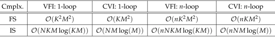
[image:28.595.60.503.212.273.2]

Table 2.1 provides the time complexity of CVI and VFI, estimated by counting the number of floating point operations. Each such operation is assumed to have complexityO(1).7 Function evaluations associated with the model primitives are also assumed to be of orderO(1).

Table 2.1: Time complexity: VFI v.s CVI

Cmplx. VFI: 1-loop CVI: 1-loop VFI:n-loop CVI:n-loop

FS O(K2M2) O(KM2) O(nK2M2) O(nKM2)

IS O(NKMlog(KM)) O(N Mlog(M)) O(nNKMlog(KM)) O(nN Mlog(M))

Note: For IS approximation, binary search is used when we evaluate the interpolating function at a given point. The results hold for linear, quadratic, cubic, andk-nearest neighbors interpolations.

For both finite space (FS) and infinite space (IS) approximations, CVI provides better performance than VFI. For FS, CVI is more efficient than VFI by order O(K), while for IS, CVI is more efficient than VFI by orderO(Klog(KM)/ log(M)). For example, if we have 250 grid points in each dimension, then in the FS case, evaluating a given number of loops will take around 250k times longer via CVI than via VFI, after adjusting for order approximations.

See appendix2.Cfor a proof of the results in table2.1.

2.5 Applications

We consider six applications. For the first two cases, we discuss optimality, con-tinuation decomposability and compare the numerical efficiency of the Bellman and Jovanovic operators. For the remaining cases, we discuss only continuation decomposability. For numerical works we apply infinite space (IS) approxima-tion withN =1000 and use linear interpolation for function approximation. All simulations of this section are processed in a standard Julia environment on a laptop witha a 2.9 GHz Intel Core i7 and 32GB RAM.8

7_{Floating point operations are any elementary actions (e.g.,}₊_,_×_,_∨_,_∧_{) on or assignments with}

floating point numbers. If f andgare scalar functions onRn, we writef(x) =O(g(x))whenever

there existC,M>0 such thatkxk ≥ Mimplies|f(x)| ≤C|g(x)|, wherek · kis the sup norm.

8_{The Julia code needed to replicate all of the applications discussed in this section,}

to-gether with alternative versions written in Python, can be found athttps://github.com/jstac/

(29)

2.5. APPLICATIONS 17

2.5.1 Job Search

Consider a worker who receives current wage offer wt and chooses to either ac-cept and work permanently at that wage, or reject the offer, receive unemploy-ment compensationc0and reconsider next period (see, e.g.,McCall(1970) or

Pis-sarides(2000)). The wage process{wt}t≥0is assumed to be

wt =ηt+θtξt, where lnθt =ρlnθt−1+lnεt (2.12)

and {ξt}, {εt} and {ηt} are positive IID innovations that are mutually indepen-dent. We interpret θt as the persistent component of labor income and allow it to be nonstationary. Whenηt is constant it can be interpreted as social security.9 Viewed as an optimal stopping problem,

• the state isz = (w,θ), with stochastic kernelPdefined by (2.12),

• the terminal reward isr(w) =u(w)/(1−β), whereuis a utility function,

• and the flow continuation rewardcis the constantu(c0).

The model is continuation decomposable, as can be seen by lettingXt :=wt and

Yt :=θt. In particular,cdoes not depend onwtand(wt+1,θt+1)is independent of

wtgivenθt. Hence the effective state space forQis one-dimensional while that of

Tis two-dimensional. Letting Fθ(w 0

,θ0) be the distribution of (wt+1,θt+1) given θt, the Bellman operator satisfies

Tv(w,θ) = max

u(w)

1−β, u(c0) +β

Z

v(w0,θ0)dFθ(w 0

,θ0)

,

while the Jovanovic operator is

Qψ(θ) = u(c0) +β

Z

max

u(w0)

1−β, ψ(θ

0₎

dFθ(w 0

,θ0).

Whether or not assumptions2.3.1–2.3.3hold depends on the primitives. Suppose for example that

u(w) = w

1−γ

1−γ with u(w) = lnw whenγ=1.

9_{Similar dynamics appear in many labor market, search-theoretic and real options studies (see}

(30)

We focus here on the case γ = 1 and 0 ≤ ρ < 1, although other cases such as γ > 1 and −1 < ρ < 0 can be treated with similar arguments.10 We take εt ∼ LN(0,σ2). Regarding assumptions2.3.1–2.3.2, we assume that {ηt}, {η_t−1} and{ξt} have finite first moments.

The reward function for this dynamic program is unbounded above and below, and the state space is likewise unbounded. Nevertheless, we can establish the key optimality results from section2.3 as follows. First, choosen ∈ N0such that βexp(ρ2nσ2) <1, and let

g(z) = g(w,θ) =θρ

n

.

To verify (2.8), we make use of the following technical lemma, which is obtained from the law of motion (2.12), and provides a bound on expected timenwages in terms of initial conditionθ0 =θ. The proof is in appendix2.B.

Lemma 2.5.1. For all n∈ N0, (a) there exist a pair An,B∈ Rsuch thatEθ|lnwn| ≤ Anθρ

n

+B, and (b)θ 7→ Eθ|lnwn|is continuous.

Now (2.8) can be established, since, conditioning onθ0 =θ,

Eθ|r(wn)| =

Eθ|lnwn|

1−β ≤

An 1−βθ

ρn₊ B

1−β =

An

1−βg(w,θ) +

B

1−β. Condition (2.9) is trivial becausec is constant. To see that condition (2.10) holds, note thatρ∈ [0, 1), so, conditioning onθ0 =θonce more,

Eθg(w1,θ1) = E (θ ρ

ε1)ρ

n =θρ

n+1

exp(ρ2nσ2/2)≤(θρ

n

+1)exp(ρ2nσ2). Hence (2.10) holds with m = d = exp(ρ2nσ2). Assumption 2.3.1 has now been established. By theorem2.3.1and proposition2.3.3,QandTare contraction map-pings with the same rate of convergence. The above analysis also implies that assumption2.3.2holds (see footnote4), so proposition2.3.4implies that bothv∗

andψ∗ are continuous.

We can also embed this problem inLp(π). To verify assumption2.3.3, we assume that the distributions of{ηt}and{ξt}are represented respectively by densitiesµ andν, and that{ηt}, {η_t−1} and{ξt}have finiteq-th moments.

Sinceρ ∈ [0, 1), the state process{(wt,θt)}has stationary density

π(w,θ) = f∗(θ)p(w|θ),

10_{One can also treat the nonstationary case}

ρ = ±1 under some further parametric

assump-tions using the weighted supremum norm techniques developed above. Details are provided in

(31)

where f∗(θ) = LN(0,σ2/(1−ρ2))andR_Ap(w|θ)dw =R_{_η₊_θξ_∈_A_}µ(η)ν(ξ)d(η,ξ). Then the next lemma (proved in appendix 2.B) implies that assumption 2.3.3

holds.

Lemma 2.5.2. The reward functions r and c are in Lq(π).

By theorem 2.3.2and proposition 2.3.5, Q and T are both contraction mappings with the same rate of convergence (in Lpnorm distances, for all 1≤ p≤q). Finally, we compare the numerical efficiency of the Bellman and Jovanovic op-erators. Table 2.2compares the time taken for CVI and VFI under different grid sizes. In tests 1–6 (50 loops), CVI is on average 261 times faster than VFI. More-over, as we increase the grid size of θ and w, computation time for VFI grows exponentially. Table2.3continues the analysis by comparing CVI and VFI under different levels of risk aversion (δ) and income persistency (ρ). Among tests 1–8 (50 loops), CVI is 267 times faster than VFI on average.

[image:31.595.111.554.489.644.2]

Recall from section2.4.2that CVI creates an orderO(Klog(KM)/ log(M))speed up over VFI for the MC algorithm. In this model, K and M are respectively the number of grid points for wt and θt. As shown in table 2.2–2.3, CVI is approx-imately K times faster than VFI in each test, which is broadly in line with the theory.

Table 2.2: Time in seconds under different grid sizes

Time & Size Test 1 Test 2 Test 3 Test 4 Test 5 Test 6

Grid size(θ,w) (200, 200) (200, 400) (300, 200) (300, 400) (400, 200) (400, 400)

Loop 10 VFI 29.70 62.47 43.78 95.19 59.47 128.73

CVI 0.325 0.176 0.259 0.268 0.361 0.348

Loop 20 VFI 58.37 125.64 87.44 190.22 118.75 257.32

CVI 0.493 0.339 0.517 0.529 0.726 0.688

Loop 50 VFI 114.38 314.30 218.62 475.78 297.34 644.57

CVI 1.014 0.824 1.277 1.289 1.786 1.757

We setρ=0.75,β= 0.95, ˜c0 =0.6,δ =1,γu =10−4,v= LN(0, 10−6)andh= LN(0, 5×10−4). The grid

points for(θ,w)lie in[10−4, 10]2.

2.5.2 Search with Learning

(32)

[image:32.595.58.502.87.241.2]

Table 2.3: Time in seconds under differentδandρvalues

Time & Value Test 1 Test 2 Test 3 Test 4 Test 5 Test 6 Test 7 Test 8

Value(δ,ρ) (2, 0.8) (2, 0.7) (2, 0.6) (3, 0.8) (3, 0.7) (3, 0.6) (4, 0.8) (4, 0.7)

Loop 10 VFI 69.75 67.86 66.61 69.80 67.68 66.70 69.96 67.84 CVI 0.205 0.161 0.163 0.375 0.394 0.386 0.372 0.371

Loop 20 VFI 139.23 135.86 133.11 139.17 135.44 132.93 139.44 135.53 CVI 0.371 0.320 0.320 0.745 0.778 0.765 0.741 0.738

Loop 50 VFI 349.08 339.84 333.24 346.93 339.10 331.86 348.84 338.53 CVI 0.866 0.834 0.794 1.908 1.894 1.895 1.850 1.837

We setβ=0.95, ˜c0=0.6,γu=10−4,v=LN(0, 10−6)andh=LN(0, 5×10−4). The grid points for(θ,w)lie in

[10−4, 10]2with 300 points each.

as in section2.5.1, except that{wt}t≥0follows lnwt =ξ+εt, where {εt}t≥0

IID

∼ N(0,δε).

Here ξ is an unobservable mean over which the worker has prior ξ ∼ N(µ,δ). The worker’s current estimate of the next period wage distribution is f(w0|µ,δ) =

LN(µ,δ+δε). If the current offer is turned down, the worker updates his belief

after observingw0. By Bayes’ rule, the posterior satisfies ξ|w0 ∼ N(µ0,δ0), where δ0 = ν(δ) :=1/(1/δ+1/δε) andµ0 = φ(µ,δ,w0) := δ0(µ/δ+lnw0/δε). Viewed

as an optimal stopping problem,

• the state isz= (w,µ,δ), and for each maph, the stochastic kernelPsatisfies

Z

h(z0)P(z, dz0) = Z

h w0,φ(µ,δ,w0),ν(δ) f(w0|µ,δ)dw0

• the reward functions arer(w) =u(w)/(1−β)andc ≡u(c0).

The model is continuation decomposable withXt :=wt andYt := (µt,δt), sincer does not depend on(µt,δt)and the next period state(wt+1,µt+1,δt+1)is indepen-dent of wt onceµt andδt are known. LettingFµ,δ(w

0_,

µ0,δ0)be the distribution of

(wt+1,µt+1,δt+1)given(µt,δt), the Bellman and Jovanovic operators are, respec-tively,

Tv(w,µ,δ) = max

u(w)

1−β, u(c0) +β

Z

v(w0,µ0,δ0)dFµ,δ(w 0

,µ0,δ0)

and Qψ(µ,δ) =u(c0) +β

Z

max

u(w0)

1−β, ψ(µ

0

,δ0)

dFµ,δ(w 0

,µ0,δ0). Again, the domain of the candidate function space is one dimension lower forQ

(33)

Regarding optimality, suppose, for example, that the CRRA parameterγis greater than 1. (The caseγ=1 can be treated along similar lines.) Letn=1 and let

g(w,µ,δ) =e(1−γ)µ+(1−γ)

2

δ/2_.

Condition (2.8) holds, since, conditioning on(µ0,δ0) = (µ,δ),

Eµ,δ|r(w1)| =

Eµ,δw 1−γ 1 1−β =

e(1−γ)2δε/2

1−β g(w,µ,δ).

Condition (2.9) is trivial sincec is constant. Condition (2.10) holds, since, condi-tioning on(µ0,δ0) = (µ,δ), the expressions ofµ0andδ0imply that

Eµ,δg(w1,µ1,δ1) = e

(1−γ)2δ1/2+(1−γ)δ1µ/δE µ,δw

(1−γ)δ1/δε

1 =g(w,µ,δ). Hence assumption2.3.1holds. Theorem2.3.1and proposition2.3.3imply thatQ

andT are contraction mappings with the same rate of convergence. The analysis above also implies that assumption2.3.2holds (see footnote4), so v∗ and ψ∗ are continuous by proposition2.3.4.

[image:33.595.113.575.533.758.2]

Finally, table 2.4 compares CVI and VFI under different grid sizes. In tests 1– 10, CVI is on average 132 times faster than VFI. In test 10, VFI takes more than 4.4 days, while CVI takes 24 minutes. Table 2.5 compares CVI and VFI under different level of risk aversion. CVI is shown to be 98 times faster than VFI on average. Again, these numerical results are close to the prediction of the theory in section2.4.2.

Table 2.4: Time in seconds under different grid sizes

Time & Size Test 1 Test 2 Test 3 Test 4 Test 5

Size(w,µ,γ) (50, 50, 50) (1, 1, 1)×102 (2, 1, 1)×102 (1, 2, 1)×102 (1, 1, 2)×102

Loop 20 VFI 685.2 5242.0 10455.1 10584.9 11443.4

CVI 14.5 61.3 60.3 134.6 131.7

Loop 50 VFI 1823.2 13020.2 26001.7 26365.2 27149.1

CVI 35.8 164.6 149.6 342.7 338.3

Time & Size Test 6 Test 7 Test 8 Test 9 Test 10

Size(w,µ,γ) (2, 2, 1)×102 (2, 1, 2)×102 (1, 2, 2)×102 (2, 2, 2)×102 (3, 3, 3)×102

Loop 20 VFI 21649.6 22267.9 21042.4 42567.8 152349.0

CVI 119.3 144.4 246.1 236.7 576.9

Loop 50 VFI 54143.5 55687.4 52578.4 106386.0 380220.0

CVI 297.0 367.8 679.2 589.9 1430.6

(34)

[image:34.595.59.480.85.220.2]

Table 2.5: Time in seconds under different risk aversion levels

Time & Value δ=1 δ=2 δ =3 δ =4 δ =5 δ =6 Mean

Loop 10 VFI 3137.1 2606.9 2615.1 2618.3 2606.5 2625.7 2701.6

CVI 25.0 25.7 30.4 30.5 30.6 30.5 28.8

Loop 20 VFI 6323.8 5206.8 5220.0 5226.9 5221.5 5242.8 5406.9

CVI 48.4 48.9 60.8 60.8 61.3 60.9 56.9

Loop 50 VFI 15976.6 13026.4 13066.7 13159.4 13099.6 13135.4 13577.3 CVI 118.9 118.9 151.9 152.3 152.8 152.6 141.2

We setβ=0.95,γε=1, and ˜c0=0.6. The grid points of(w,µ,γ)lie in[10−4, 10]×[−10, 10]×[10−4, 10] with(100, 100, 100)points.

2.5.3 Firm Entry

Consider a condensed version of the firm entry problem in Fajgelbaum et al.

(2017). At the start of period t, a firm observes a fixed cost ft and then decides whether to incur this cost and enter a market, earning stochastic payoff πt, or wait and reconsider next period. The sequence{ft}isIID, while the current pay-off πt is unknown prior to entry. The firm has prior beliefφ(π;θt), where φis a distribution over payoffs that is parameterized by a vectorθt. If the firm does not enter thenθt is updated via Bayesian learning. In an optimal stopping format,

• the state isz= (f,θ), with stochastic kernelPdefined by the distribution of {ft}and the Bayesian updating mechanism of{θt},

• the terminal reward is the entry payoffr(f,θ) = R πφ(dπ;θ)− f,

• and the flow continuation rewardc ≡0.

This model is continuation decomposable, as can be seen by lettingXt := ft and

Yt := θt. In particular, since{ft}is IID,(ft+1,θt+1) is independent of ft given θt. Let Fθ(f

0_,

θ0)be the distribution of(ft+1,θt+1)givenθt. The Bellman operator is

Tv(f,θ) = max

Z

πφ(dπ;θ)−f, β

Z

v(f0,θ0)dFθ(f 0

,θ0)

,

while the Jovanovic operator is

Qψ(θ) = β

Z

max

Z

πφ(dπ;θ0)− f0, ψ(θ0)

dFθ(f 0

(35)

2.5.4 Research and Development

Firm’s R&D decisions are often modeled as a sequential search process for better technologies (see, e.g., Jovanovic and Rob(1989), Bental and Peled (1996), Perla and Tonetti (2014)). Each period, an idea of value st is observed, and the firm decides whether to put this idea into productive use, or develop it further by in-vesting in R&D. The former choice yields a payoffr(st,kt), wherektis the amount of capital input. The latter incurs a fixed costc0 >0 (that renderskt+1 = kt−c0) and creates a new technology st+1 next period. Let {st} IID∼ µ. Viewed as an optimal stopping problem,

• the state isz = (s,k), and for given maph, the stochastic kernelPsatisfies

Z

h(z0)P(z, dz0) = Z

h s0,k−c0

µ(ds0),

• the terminal reward isr(s,k)and the flow continuation reward isc ≡ −c0.

This model is also continuation decomposable, as can be seen by lettingXt :=st andYt :=kt. LetFk(s0,k0)be the distribution of(st+1,kt+1)givenkt. The Bellman and Jovanovic operators are respectively

Tv(s,k) =max

r(s,k),−c0+β

Z

v(s0,k0)dFk(s0,k0)

and Qψ(s) = −c0+β

Z

maxr(s0,k0),ψ(s0) dFk(s0,k0).

2.5.5 Real Options

Consider a general financial/real option framework (see, e.g.,Dixit and Pindyck

(1994),Alvarez and Dixit(2014), andKellogg(2014)). Letptbe the current price of a certain financial/real asset andλtanother state variable. The process{λt}isΦ -Markov and affects{pt}via pt = f(λt,εt), where{εt} IID∼ µ and is independent of {λt}. Let K be the strike price of the asset. Each period, the agent decides whether to exercise the option now (i.e., purchase the asset at price K), or wait and reconsider next period. In an optimal stopping format,

• the state isz = (p,λ), and for given maph, the stochastic kernelPsatisfies

Z

h(z0)P(z, dz0) = Z

(36)

• the terminal reward (exercise the option now) isr(p) = (p−K)+,

• and the flow continuation reward isc≡0.

The model is continuation decomposable, with Xt := pt and Yt := λt. Let

Fλ(p 0

,λ0) be the distribution of(pt+1,λt+1) conditional on λt. The Bellman and Jovanovic operators are, respectively,

Tv(p,λ) =max

(p−K)+,β

Z

v(p0,λ0)dFλ(p 0

,λ0)

and Qψ(λ) = β

Z

max(p0−K)+,ψ(λ0) dFλ(p 0

,λ0).

2.5.6 Transplants

In health economics, a well-known problem concerns the decision of a surgeon to accept/reject a transplantable organ for the patient (see, e.g., Alagoz et al.,

2004). The surgeon aims to maximize the reward of the patient. Each period, she receives an organ offer of qualityqt, where {qt} IID∼ G. The patient’s health

ht evolves according to a H-Markov process if the surgeon rejects the organ. If she accepts this organ for transplant, the operation succeeds with probability

p(qt,ht), and confers benefitB(ht) to the patient, while a failed operation results in death. The patient’s single period utility when alive is u(ht). Viewed as an optimal stopping problem,

• the state isz= (q,h), and for a given map f, the stochastic kernelPsatisfies

Z

f(z0)P(z, dz0) = Z

f(q0,h0)G(dq0)H(h, dh0),

• the terminal reward (accept the offer) isr(q,h) = u(h) +p(q,h)B(h),

• and the flow continuation reward isc(h) = u(h).

This model is continuation decomposable by letting Xt := qt and Yt := ht. Let

Fh(q0,h0)be the distribution of (qt+1,ht+1) given ht. The Bellman and Jovanovic operators are respectively

Tv(q,h) =max

u(h) +p(q,h)B(h), u(h) +β

Z

v(q0,h0)dFh(q0,h0)

and Qψ(h) = u(h) +β

Z

(37)

2.A. SOME LEMMAS 25

Appendix 2.A

Some Lemmas

To see the symmetric properties of Qand T from an alternative perspective, we start our analysis with a generic candidate continuation value function space. Let

C be a subset ofmB such thatψ∗ ∈ C and QC ⊂C. LetV be defined by

V :=RC ={v∈ mB: v=r∨ψ for someψ∈C}. (2.A.1)

Then R is a surjective map from C onto V, Q = LR on C and T = RL on V. The following result parallels the theory of section2.3.1, and is helpful for deriv-ing important convergence properties once topological structure is added to the generic setting, as to be shown.

Lemma 2.A.1. The following statements are true: (1) LV ⊂C and TV ⊂V.

(2) If v is a fixed point of T inV, then Lv is a fixed point of Q inC.

(3) Ifψis a fixed point of Q inC, then Rψis a fixed point of T inV.

(4) Tt+1 =RQtL onV and Qt+1 =LTtR onC for all t∈ N₀.

Proof. The proof is similar to that of propositions2.3.1–2.3.2and thus omitted. Lemma 2.A.2. Under assumption2.3.1, there exist b1,b2 ∈ R+ such that for all z∈ Z,

(1) |v∗(z)| ≤ _∑n_t₌−₀1βtEz[|r(Zt)|+|c(Zt)|] +b1g(z) +b2.

(2) |ψ∗(z)| ≤_∑n_t₌−₁1βtEz|r(Zt)|+∑_tn=−01βtEz|c(Zt)|+b1g(z) +b2.

Proof. Without loss of generality, we assumem 6=1 in assumption2.3.1. By that assumption, Ez|r(Zn)| ≤ a1g(z) +a2, Ez|c(Zn)| ≤ a3g(z) +a4 and Ezg(Z1) ≤

mg(z) +dfor allz ∈Z. For allt≥1, by the Markov property (see, e.g.,Meyn and Tweedie(2009), section 3.4.3),

Ezg(Zt) = Ez[Ez(g(Zt)|Ft−1)] =Ez EZt−1g(Z1)

≤mEzg(Zt−1) +d. Induction shows that for allt≥0,

Ezg(Zt) ≤mtg(z) +1 −mt

1−md. (2.A.2)

Moreover, for allt≥n, applying the Markov property again yields

Ez|r(Zt)|=Ez[Ez(|r(Zt)||Ft−n)] =Ez EZt−n|r(Zn)|

(38)

26 2.A. SOME LEMMAS

By (2.A.2), for allt≥n, we have

Ez|r(Zt)| ≤a1

mt−ng(z) +1−m

t−n

1−m d

+a2. (2.A.3)

Similarly, for allt≥n, we have

Ez|c(Zt)| ≤ a3Ezg(Zt−n) +a4 ≤a3

mt−ng(z) +1−m

t−n

1−m d

+a4. (2.A.4)

Let S(z) := ∑_t_≥₁βtEz[|r(Zt)|+|c(Zt)|]. Based on (2.A.2)–(2.A.4), we can show that

S(z)≤ n−1

∑

t=1

βtEz[|r(Zt)|+|c(Zt)|] + a1

+a3

1−βm g(z) +

(a1+a3)d+a2+a4

(1−βm)(1−β) . (2.A.5) Since|v∗| ≤ |r|+|c|+Sand |ψ∗| ≤ |c|+S, the two claims hold by lettingb1 :=

a1+a3

1−βm andb2 :=

(a1+a3)d+a2+a4

(1−βm)(1−β) .

Lemma 2.A.3. Under assumption2.3.1, the value function solves the Bellman equation

v∗(z) =max

r(z), c(z) +β

Z

v∗(z0)P(z,dz0)

=max{r(z), ψ∗(z)}.

Proof of lemma2.A.3(method 1). By theorem 1.11 ofPeskir and Shiryaev(2006), it suffices to show that Ez

sup_k_≥₀

∑

k−1

t=0 βtc(Zt) +βkr(Zk)

< ∞ for all z ∈ Z. This is true since with probability one we have

sup k≥0

k−1

∑

t=0

βtc(Zt) +βkr(Zk)

≤

∑

t≥0

βt[|r(Zt)|+|c(Zt)|], (2.A.6)

and by the monotone convergence theorem and lemma 2.A.2(see (2.A.5) in ap-pendix2.A), the right hand side of (2.A.6) isPz-integrable for allz∈ Z.

(39)

2.B. MAIN PROOFS 27

Appendix 2.B

Main Proofs

Proof of theorem2.3.1. Let d1 := a1+a3 and d2 := a2+a4. Since βm < 1 by as-sumption2.3.1, we can choose positive constantsm0 andd0such that

m+d1m0 >1, ρ:=β(m+d1m0) <1 and d0 ≥(d2m0+d)/(m+d1m0−1). (2.B.1) Regarding claim (1), we first show that Q is a contraction mapping on b`Zwith

modulusρ. By the weighted contraction mapping theorem (see, e.g.,Boyd(1990), section 3), it suffices to verify: (a) Q is monotone, i.e., Qψ ≤ Qφ if ψ,φ ∈ b`Z

and ψ ≤ φ; (b) Q0 ∈ b`Z and Qψ is B-measurable for all ψ ∈ b`Z; and (c) Q(ψ+a`) ≤ Qψ+aρ` for all a ∈ R+ and ψ ∈ b`Z. Obviously, condition (a)

holds. By (2.5) and (2.11), we have |(Q0)(z)|

`(z) ≤

|c(z)|

`(z) +β

Z |_r₍_z0₎|

`(z) P(z,dz

0₎ _≤₍

1+β)/m0 <∞

for allz ∈ Z, sokQ0k` <∞. The measurability ofQψfollows immediately from

our primitive assumptions. Hence, condition (b) holds. By the Markov property (see, e.g.,Meyn and Tweedie(2009), section 3.4.3), we have

Z

Ez0|r(Zt)|P(z, dz0) =Ez|r(Zt+1)| and

Z

Ez0|c(Zt)|P(z, dz0) = Ez|c(Zt+1)|.

Leth(z):=∑n_t₌−₁1Ez|r(Zt)|+∑n_t=−01Ez|c(Zt)|, then we have

Z

h(z0)P(z, dz0) =

n

∑

t=2

Ez|r(Zt)|+ n

∑

t=1

Ez|c(Zt)|. (2.B.2)

By the construction ofm0andd0, we havem+d1m0 >1 and(d2m0+d+d0)/(m+

d1m0)≤d0. Assumption2.3.1and (2.B.2) then imply that

Z

κ(z0)P(z,dz0) = m0 n

∑

t=1

Ez[|r(Zt)|+|c(Zt)|] +

Z

g(z0)P(z,dz0) +d0

≤m0

n−1

∑

t=1

Ez[|r(Zt)|+|c(Zt)|] + (m+d1m0)g(z) +d2m0+d+d0

≤(m+d1m0)

m0 m+d1m0

h(z) +g(z) +d0

≤(m+d1m0)`(z). (2.B.3)

Since` ≤κ, this implies that for allz ∈Z, we have

Z

κ(z0)P(z, dz0)≤(m+d1m0)κ(z) and

Z

(40)

28 2.B. MAIN PROOFS

Hence, for allψ∈ b`Z,a ∈R+andz ∈Z, we have

Q(ψ+a`)(z) =c(z) +β

Z

maxr(z0),ψ(z0) +a`(z0) P(z,dz0) ≤c(z) +β

Z

maxr(z0),ψ(z0) P(z,dz0) +aβ

Z

`(z0)P(z,dz0)

≤Qψ(z) +aβ(m+d1m0)`(z) = Qψ(z) +aρ`(z).

So condition (c) holds, andQ: b`Z→b`Zis a contraction mapping of modulusρ. Moreover, lemma 2.A.3and the analysis related to (2.4) imply thatψ∗ is indeed a fixed point of Qunder assumption 2.3.1. Lemma2.A.2implies that ψ∗ ∈ b`Z.

Hence,ψ∗must coincide with the unique fixed point ofQunderb`Z, and claim (1)

holds.

The proof of claim (2) is similar. In particular, using (2.B.4) one can show that

T : bκZ → bκZ is a contraction mapping of the same modulus. We omit the

details.

Proof of proposition2.3.4. Let b`cZbe the set of continuous functions inb`Z. Since

`is continuous by assumption2.3.2,b`cZis a closed subset ofb`Z(see e.g.,Boyd

(1990), section 3). To show the continuity ofψ∗, it suffices to verify thatQ(b`cZ) ⊂ b`cZ (see, e.g., Stokey et al. (1989), corollary 1 of theorem 3.2). For fixed ψ ∈

b`cZ, let h(z) := max{r(z),ψ(z)}, then there exists G ∈ R+ such that |h(z)| ≤ |r(z)|+G`(z) =: ˜h(z). By assumption 2.3.2, z 7→ h˜(z)±h(z) are nonnegative and continuous. For allz∈ Zand{zm} ⊂ Zwithzm →z, the generalized Fatou’s lemma ofFeinberg et al.(2014) (theorem 1.1) implies that

Z

˜

h(z0)±h(z0)

P(z, dz0) ≤lim inf m→∞

Z

˜

h(z0)±h(z0)

P(zm, dz0).

Since limm→∞R h˜(z0)P(zm, dz0) =R h˜(z0)P(z, dz0)by assumption2.3.2, we have

±

Z

h(z0)P(z, dz0) ≤lim inf m→∞

±

Z

h(z0)P(zm, dz0)

,

where we have used the fact that for all sequences {am} and {bm} in R with lim

m→∞am exists, we have: lim infm→∞ (am +bm) = mlim→∞am+lim infm→∞ bm. Hence,

lim sup m→∞

Z

h(z0)P(zm, dz0)≤

Z

h(z0)P(z, dz0)≤lim inf m→∞

Z

h(z0)P(zm, dz0), (2.B.5)

i.e., z 7→ R

h(z0)P(z, dz0) is continuous. Since c is continuous by assumption,

Qψ ∈ b`cZ. Hence, Q(b`cZ) ⊂ b`cZand ψ∗ is continuous, as was to be shown. The continuity of v∗ follows from the continuity of ψ∗ and r and the fact that

Continuation Value Methods for Sequential Decisions: A General Theory