A deep learning framework for joint image restoration and recognition

recognition

.

White Rose Research Online URL for this paper:

http://eprints.whiterose.ac.uk/148223/

Version: Published Version

Article:

Chen, R., Mihaylova, L. orcid.org/0000-0001-5856-2223, Zhu, H. et al. (1 more author)

(2019) A deep learning framework for joint image restoration and recognition. Circuits,

Systems and Signal Processing. ISSN 0278-081X

https://doi.org/10.1007/s00034-019-01222-x

[email protected] https://eprints.whiterose.ac.uk/

Reuse

This article is distributed under the terms of the Creative Commons Attribution (CC BY) licence. This licence allows you to distribute, remix, tweak, and build upon the work, even commercially, as long as you credit the authors for the original work. More information and the full terms of the licence here:

https://creativecommons.org/licenses/

Takedown

If you consider content in White Rose Research Online to be in breach of UK law, please notify us by

https://doi.org/10.1007/s00034-019-01222-x

A Deep Learning Framework for Joint Image Restoration

and Recognition

Ruilong Chen1·Lyudmila Mihaylova1 ·Hao Zhu2· Nidhal Carla Bouaynaya3

Received: 1 September 2018 / Revised: 5 July 2019 / Accepted: 6 July 2019 © The Author(s) 2019

Abstract

Image restoration and recognition are important computer vision tasks representing an inherent part of autonomous systems. These two tasks are often implemented in a sequential manner, in which the restoration process is followed by a recognition. In contrast, this paper proposes a joint framework that simultaneously performs both tasks within a shared deep neural network architecture. This joint framework inte-grates the restoration and recognition tasks by incorporating: (i) common layers, (ii) restoration layers and (iii) classification layers. The total loss function combines the restoration and classification losses. The proposed joint framework, based on capsules, provides an efficient solution that can cope with challenges due to noise, image rota-tions and occlusions. The developed framework has been validated and evaluated on a public vehicle logo dataset under various degradation conditions, including Gaussian noise, rotation and occlusion. The results show that the joint framework improves the accuracy compared with the single task networks.

Keywords Capsule networks·Image restoration·Image recognition·Deep neural networks

B

[email protected]

Ruilong Chen

[email protected]

Hao Zhu

[email protected]

Nidhal Carla Bouaynaya [email protected]

1 _{Department of Automatic Control and Systems Engineering, The University of Sheffield,}

Sheffield S1 3JD, UK

2 _{Chongqing University of Posts and Telecommunications, Chongqing 400065,}

People’s Republic of China

1 Introduction

Image recognitionis an important field, especially for autonomous systems. The field witnessed new opportunities and became very popular with the development of con-volutional network networks (CNNs) in 2012 [15]. Before the creation of CNNs, the majority of image recognition approaches included a hand-crafted feature detection and feature description process [15,17]. Optimization algorithms for nonconvex data and image restoration are proposed in [4,5]. Compressed sensing algorithms incopro-rating second-order derivatives in efficient ways are developed in [6], approaches based on conjugate priors in [7] and on supporting machines in [19]. In such approaches, image features are extracted at pixel level or regional level and then embedded in the recognition process [32]. Unlike traditional hand-crafted feature methods, such as the scale-invariant feature transform (SIFT) [17], CNNs automatically detect the image features by multiple convolutional and nonlinear operations. However, a CNN has a large number of parameters to learn, which requires large datasets.

Image restoration, on the other hand, aims to recover a clear image from its noisy, rotated and occluded version that the sensor provides. It is known as an ill-posed inverse problem [18] and has been a focus of significant research. The majority of works consider a super-resolution single image and its denoising. For example, the total variation [20] and BM3D algorithm [3] achieve good performance over single image denoising. The algorithms reported in [10,14,27,30] achieve state-of-the-art performance on a single image with super-resolution [9]. However, these methods are only applicable to particular types of image degradation. For example, the BM3D approach is designed only for image denoising.

Deep learning methods extract image features from groups of images and hence can be used for both image denoising and image restoration. In fact, deep neural networks take advantage of the availability of big data and the automatic learning process, which outperforms traditional image restoration methods [9,18]. Recently, deep neural networks have been developed for the purpose of image restoration. For example, Mao et al. [18] proposed a CNN architecture that could perform image denosing and construct super-resolution images. Being purely data driven, the approaches for learning restoration are promising as they do not need models nor assumptions about the nature of the degradation [18].

1.1 Related Convolutional Neural Network Approaches

Lecun et al. proposed the first CNN architecture, called LeNet [16], which lays down the beginning of the development of CNN architectures able to deal with big volumes of data and more and more complex inference tasks. Next, AlexNet achieved the best performance on ImageNet in 2012. Subsequently, different CNN architectures were developed rapidly and achieved higher than human performance on datasets, such as ImageNet [15].

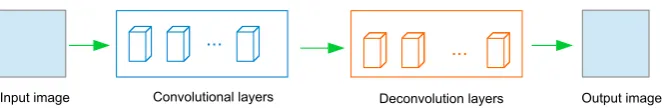
Fig. 1 A typical restoration architecture based on CNNs

with neural networks. Therefore, it can prevent the over-fitting problem, which is one of the main challenges in neural networks [25]. The CNN architectures are mainly composed of convolution operations, followed by nonlinearity (activation functions) and pooling operations.

The ZF-Net [31] architecture applies a smaller kernel size than AlexNet in the first layer. The reason behind this modification is that a smaller size in the first convolutional layer helps retain more original pixel information in the input volume. A large filtering size, e.g.,[11×11], proved to be skipping relevant information from the input. ZF-Net achieved a smaller error rate than AlexNet on ImageNet [8].

The VGG-NET architechture [24] further enhances the depth of the CNNs up to 19 layers and uses a unique kernel size of[3×3]. Google-Net [26] model increases the number of layers to 22 and applies an inception module, in which different convolu-tional feature maps, generated by convoluconvolu-tional kernels of different sizes, are combined at every layer. The Res-Net [11], built up with a 152-layer architecture, introduces the idea of residual learning, which builds shortcut connections between layers to miti-gate the vanishing gradient problem and improve the optimization process. In 2015, Res-Net achieved the best accuracy on ImageNet.

Figure 1 shows the generic coding–decoding architecture of a CNN for image restoration [18]. The restoration framework is based on the typical convolutional operations of CNNs. The main difference is the lack of pooling and fully connected layers in the restoration process. The developed CNN approaches for restoration and recognition differ significantly from each other. The recognition process discards infor-mation, layer by layer, and finishes the process by providing a representative feature vector that is fed to neurons in the last fully connected layer. TheCNNs for recognition

discard information to extract the most representative feature in an image, while CNNs for restoration need to keep detailed information of the ground truth. In particular, the pooling process is not appropriate for restoration.

However, these networks and other state-of-the-art networks, such as RED-Net [18], VGG [24] and ResNet [11], face difficulties in dealing with image occlusion, rotation, denoising and super-resolution. This motivated us to develop efficient image restoration methods that particularly deal with rotation and occlusion. In addition, it would be beneficial if the restoration and recognition share a framework, which could jointly perform both tasks, rather than in a sequential manner (restoration followed by recognition).

represents the probability of the object’s (or part of the object) existence, and the orientation represents the instantiation parameters [21]. Previous works [2,21] show that the capsule network approach achieves better results on image recognition than conventional CNNs.

The main contributions of this work can be summarized as follows: 1) A deep learning architecture for joint image restoration and recognition is proposed based on capsules and conventional CNNs; 2) a new multi-loss function that combines the restoration and classification losses is proposed. A hyper-parameter is used to control the trade-off between the two loss functions. The linear combination of the restoration and classification losses can be viewed as a form of regularization as it constrains the search space for possible candidate solutions for each individual task; 3) a capsule CNN is proposed to handle image restoration from rotation and occlusion; 4) the developed framework is validated and its performance is evaluated using a public dataset.

The rest of this paper is organized as follows. Section2introduces the principles of the generic CNN and capsule network. Section3presents the developed joint frame-work for image restoration and recognition based on CNNs and capsule netframe-works. Section4gives detailed evaluation of the performance of the proposed deep learning framework compared with state-of-the-art approaches. Finally, Sect.5summarizes the results.

2 Theoretical Background for Convolutional and Capsule Neural

Networks

2.1 The Convolutional Neural Network Approach

Convolutional layers extract image feature maps by using different convolutional ker-nels. Suppose thatn convolutional kernels are used in thekt h layer. Then theit h,

i =1,2, . . . ,n, convolutional feature map in the(k+1)layer can be denoted as:

I_ik+1= f

⎛

⎝

j

Vi∗Ikj

⎞

⎠, (1)

whereIj is the jt hfeature map andVi is theit hkernel. Here,Ijcan be a channel of the original image, a pooling map or a convolutional map, f(·)denotes a nonlinear activation function and∗represents the convolution operation. The Rectified Linear Unit (ReLU) with the following nonlinear functiong(x)=max(0,x)is often used [15] in CNNs.

A pooling process often decreases the size of the input feature maps. Hence, pooling can be regarded as a down-sampling operation. Each pooling map in layerk+1 is obtained by a pooling operation over the corresponding feature maps in the previous layerkand is given as follows:

Iik+1=pool(I k

where the indexigoes though all maps in layerkand pool(·)represents the pooling method. A window shifts on the previous maps, and the mean value (or the maximum value) in each window is extracted to form a pooling map. The convolution and pooling operations are the two main operations in CNNs. The last layer is reshaped to a vector form and then fully connected with neurons in the same way as in generic neural networks. The loss functionLcla, typically used in image recognition, is the

cross-entropy function and is defined as follows:

Lcla =

i

−yiln(yˆi)−(1−yi)ln(1− ˆyi)

, (3)

whereyandyˆare, respectively, the ground truth label and the predicted label vectors for an image in the one-hot coded manner (a one-hot vector contains only one value equal to 1 and all other elements are zero valued), with theit hentry denoted asyi and

ˆ

yi.

2.2 The Capsule Network Approach

Connections between layers are of scalar-scalar type in generic CNNs. In acapsule network [21], neurons are combined in a group to represent an entity or part of an entity. In particular, a neuron is replaced with a group of neurons and the connections between capsule layers become of vector–vector type. For each capsule (represented as a vector), anonlinear squash function f(·)is defined:

f(x)= ||x||

2 2

1+ ||x||2 2

x

||x||2

, (4)

withxbeing the input vector of the squash function and|| · ||2denotes thel2-norm.

This function makes the length of short vectors shrink close to 0 and long vectors expand close to 1. Hence, the output length can be used to represent the probability that an entity exists. The outputvj of the j-th capsule is given by:

vj = f(hj), (5)

wherehj is the input of the j-th capsule. The parameters of each capsule represent various properties such as position, scale and orientation of a particular entity [21].

Except for the capsules in the first capsule layer, the total inputhjof thej-th capsule is a weighted sum:

hj =

i

ci joj|i, (6)

Letqi j denote the log prior probabilities that capsulei (in the previous layer) is coupled with capsulej(in the current layer). The coefficientsci jcan then be expressed as:

ci j =

exp(qi j)

dexp(qi d)

, (7)

where the indexd refers to all capsules in the current layer.qi js are initialized with zeros and updated by a routing algorithm. In the routing algorithm,qi j is updated by the following process:

q_{i j}(r+1)=q_{i j}(r)+

vj,oj|i, (8)

where r is an iteration index. The term

vj,oj|i is the inner product between the predicted output and its actual output (of capsulejin the current layer). The assumption is intuitive since all capsules from the previous layer will predict the value of capsule

j in the current layer. If the prediction made by capsulei from the previous layer is similar to the actual outputvj, capsule i should have a high probability of the contribution; Hence, the coupling coefficientci j increases.

In Eqs. (6) and (8), the predictionsoj|i can be calculated by the output capsulesui from the previous layer:

oj|i =Wi jui, (9)

where Wi j are transformation matrices connecting capsules between two adjacent layers. Suppose there areCclasses, then the final capsule layer hasCcapsules, with the length of each capsule representing the existence probability of the corresponding object. To allow multiple classes in the same image to exist, a margin loss function is used, with the loss functionLifor classi (i =1,2, . . . ,C) given by:

Li =yimax(0,m+− ||vi||2)2+λ(1−yi)max(0,||vi||2−m−)2, (10)

where||vi||2is the length of the vectorviin the final capsule layer andyi =1 if and only if the object of classiexists. This leads the length of capsulevi to be abovem+ if an object of classiis present and induces the length of capsulevi to be belowm− when an object of classi is absent. Here,λis a controlling parameter and the total classification loss function is calculated byLcla = iLi, which simply sums the losses from all the final layer capsules.

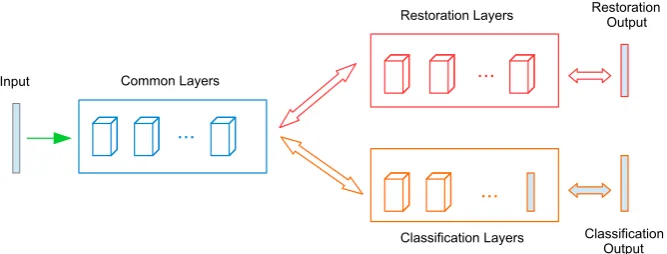
Fig. 2 A general joint framework for image restoration and recognition

3 A Joint Framework for Image Restoration and Recognition

Conventional methods [28] use the restoration and recognition pipeline, in which a restoration stage is followed by a recognition process [1]. However, a joint framework that simultaneously performs restoration and recognition would be more efficient. Figure2illustrates the general architecture of a joint framework. The proposed joint framework can remove noise, correct a rotated image, recover an occluded image and perform recognition. This joint framework integrates the restoration and recognition tasks by incorporating (i) common layers, (ii) restoration layers and (iii) classification layers. The total loss function combines the classification and restoration losses. For each input image, the restoration error function is given by:

Lres=

1

nm

n

i=1

m

j=1

(R(i,j)−I(i,j))2, (11)

whereR(i,j)is the predicted value at location index(i,j)in the last restoration layer andI(i,j)is the ground truth training image intensity at location index(i,j).

The gradient descent method is then applied to minimize Lres andLcla for the

three-pathway framework. Hence, the total loss function is given as:

Ltotal=βLcla+(1−β)Lrec, (12)

Algorithm 1Training process of a joint framework

Require:

The original training images and labels.

The designed joint framework. The image degradation parameters.

Ensure:

Randomly initialize the convolutional kernels. Separate the training data into small batches. 1:fori t er ati on i ndex=1,i t er ati on i ndex++do

2: forbat ch i ndex=1,bat ch i ndex++do

3: Contaminate the source image with image degradations, such as rotation and occlusion. 4: Run the network forward using the degraded images.

5: Calculate the total loss.

6: Calculate the gradient of all the weights and update the weights. 7: end for

8: Decrease the learning rate. 9:end for

10:return The weights in the common layers, restoration layers and classification layers.

3.1 A Joint Restoration–Recognition Convolutional Neural Network Framework

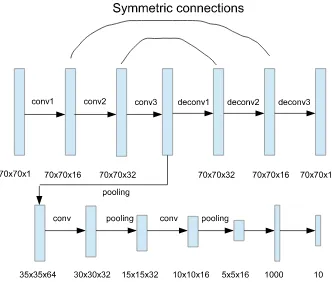
The proposed joint restoration–recognition CNN framework is illustrated in Fig.3. The framework comprises three common layers, three restoration layers and five clas-sification layers (three pooling layers and two convolutional layers). In order to keep the size of the input image after convolution, kernels of size[11×11]are applied to all the common and restoration layers with a padding size of[5×5]. Symmetric connections are applied by setting gate factors to 0.1 and 0.2 on conv1 and conv2, respectively [18].

For recognition, two convolutional layers and three max-pooling layers are applied. Convolutional kernels of size[6×6]without padding are applied. A fully connected layer is then connected with the output label. The softmax function is applied in the last stage of the classification. Hence, the output represents the probability of the input data belonging to the corresponding class.

Notice that the loss function for image restoration is calculated as the average pixelwise difference between the ground truth images and predicted images. Such a definition is sensitive to image rotation, as rotation can involve a huge variation in the loss function without changing the image content. In fact, rotation is known to seriously influence the classification accuracy in CNNs [13,22].

3.2 A Joint Framework Based on Capsule Networks

Fig. 3 The joint CNN framework for image restoration and recognition

measurement. In the last fully connected capsule layer, weights are optimized by the margin loss function given in Eq. (10).

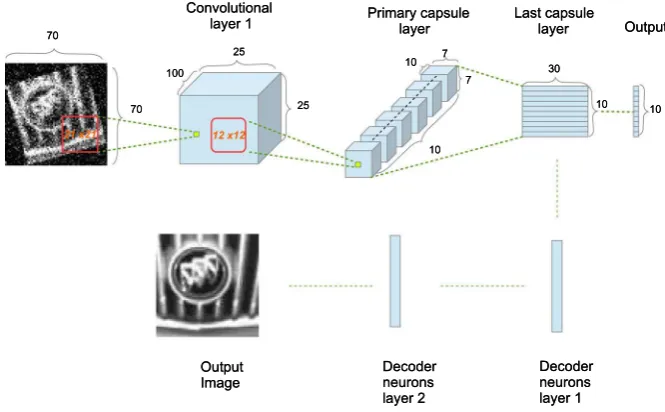
The capsule network has a decoder process that allows the reconstruction of the input image. Hence, the weights are not only updated by the classification but also depend on the reconstruction loss function. The capsule network can be transformed for image restoration in the following way: Feed the corrupted images as the input and calculate the loss between the ground truth images and the restored images. In such a way, the joint framework automatically learns the weights based on the ground truth images. Figure4illustrates the architecture of the joint image restoration and recognition framework based on capsule networks.

4 Performance Evaluation

Fig. 4 The joint capsule framework for image restoration and recognition

Fig. 5 Twenty test images for illustration purpose

The architecture given in Fig.3is the designed joint CNN architecture (Joint-CNN-Net). In order to present a comparison with state-of-the-art networks, we extend the RED-Net [18] by adding two fully connected layers for recognition (the same as last two recognition layers in Joint-CNN-Net) after the conv layers, while keeping the restoration network the same as in RED-Net10. RED-Net has similarities with the well-know recognition networks VGG [24] for the network structure and ResNet [11] for the symmetric skip connections.

In the proposed capsule Joint-Cap-Net framework, shown in Fig. 4, three itera-tions are applied in the routing process. The performance evaluation of all networks is conducted in Python with the PyTorch toolbox on a laptop with the following spec-ifications: Intel CPU I5 and Nvidia GTX 1070 (extended GPU). The performance of each model is measured in terms of accuracy (percentage of correctly classified images) on the entire test dataset (1500 images).

Joint-CNN-0 1e-6 1e-5 1e-4 1e-3 0.01 0.05 0.1 0.2 0.3 0.4 0.5 0.6 0.7 0.8 0.9 0.95 0.99 0.999(1-e-4)(1-e-5) 1 values 0 20 40 60 80 100 Accuracy (%) 8 10 12 14 16 18 20 22 24 PSNR Value

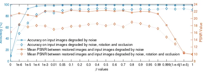
Accuracy on input images degraded by noise

Accuracy on input images degraded by noise, rotation and occlusion Mean PSNR between restored images and input images degraded by noise

Mean PSNR between restored images and input images degraded by noise, rotation and occlusion

Fig. 6 Validation with different values ofβusing the Joint-Cap-Net on images degraded only by noise, and images degraded by combing effects from noise, rotation and occlusion

Net, around 1 min for Joint-Red-Net and Joint-Cap-Net. During the testing phase, the evaluation over 1,500 images took 3.29s for the Joint-CNN-Net, 2.54s for Joint-RED-Net and 1.46s for the Joint-Cap-Joint-RED-Net.

In this section, the Joint-CNN-Net and the Joint-Cap-Net are evaluated under var-ious degradation conditions including noise, rotation and occlusion. Their accuracy is evaluated using the model generated at the 100-th epoch in the training stage. The peak signal-to-noise ratio (PSNR), in [dB], and the structural similarity (SSIM) index [29] are used to compare each original test image with its degraded version (O-D) and its recovered version (O-R). The PSNR (the higher the better) and SSIM (ranges from

−1 to 1, the higher the better) are measures for comparing the differences between two images. The PSNR focuses on the difference between the pixel-pixel intensity values and the SSIM considers the structures within an image [23].

4.1 Trade-Off Between Restoration and Recognition Performance

A natural question to ask is how the joint framework would change the performance of restoration and recognition when compared with the individual implementation of each task. It is a generic framework that achieves a trade-off between restoration and classification by setting different values of the hyper-parameterβ. For example, if β = 1, the joint framework is purely a recognition framework. On the contrary, a purely restoration framework could be built by settingβ =0, in which recognition is no longer considered in the weight updating process. In order to test the trade-off between the results from these two tasks, values ofβ are evaluated in the range of

[0,1].

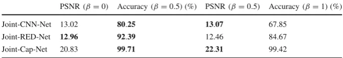
Table 1 Evaluations of single task networks and joint frameworks

PSNR(β=0) Accuracy(β=0.5)(%) PSNR(β=0.5) Accuracy(β=1)(%)

Joint-CNN-Net 13.02 80.25 13.07 67.85

Joint-RED-Net 12.96 92.39 12.46 84.67

Joint-Cap-Net 20.83 99.71 22.31 99.42

The bold indicates the best performance in terms of accuracy, PSNR and SSIM

than 0.001. For restoration, the PSNR tends to drop quickly whenβ is larger than 0.95. Variations in accuracy and PNSR whenβ is in the range of [0.05, 0.95] can be explained by the uncertainties due to noise, the random rotations and occlusions. In addition, there is no evidence that the restoration and recognition architectures could achieve better results by setting β = 1 and β = 0, respectively. On the contrary, involving a classification loss function gives better results than without it for most of theβvalues. Figure6shows high accuracy and significant restoration results whenβ is in the range of[0.05,0.95]. Hence, in the following experiments,β is set equal to 0.5.

This paper has also built two other joint frameworks based on CNNs and compared them with the single task network by settingβ =0 as a restoration network andβ =1 for the recognition network. Table1presents results from the comparison of the pure recognition network (β =1), pure restoration network (β =0) and joint framework (β =0.5) for Joint-CNN-Net, Joint-RED-Net and Joint-Cap-Net. Table1shows that joint frameworks improve the accuracy compared with the single task networks.

The proposed joint architecture is flexible and can embed a state-of-the-art single task network either for recognition or for restoration. By sharing common layers, the joint framework demonstrates better performance when compared with single task networks. For example, Table1shows that the joint frameworks increase the recog-nition accuracy by 12.4%, 7.72% and 0.29% for Joint-CNN-Net, Joint-RED-Net and Joint-Cap-Net, respectively. For image restoration, the PSNR increased significantly for Joint-Cap-Net and slightly dropped from 12.96 to 12.46 for Joint-RED-Net.

4.2 Robustness Evaluations

4.2.1 Noise Robustness Evaluation

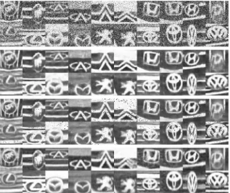
Fig. 7 First 2 rows: Noisy images. Restored images by Joint-CNN-Net, Joint-RED-Net and Joint-Cap-Net, respectively

By comparing these restored images with their corresponding ground truth, as shown in Fig. 5, it is evident that some of the images recovered by Joint-Cap-Net have even better visual quality than the ground truth. For example, the two ground truth “Lexus” images have a slight noise inside, while the Joint-Cap-Net removes this noise in the recovered images. For the image denoising task, both the Joint-Cap-Net and Joint-CNN-Joint-Cap-Net frameworks achieve good results. The denoising results from these two frameworks are similar. Notice that the Joint-Cap-Net automatically rotates images, for example, the last “VW” image has been rotated. These are due to the 2D convolutional kernels preserving the spatial information in CNNs, while the capsules are not restricted to pixel-to-pixel recovery.

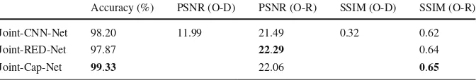
Table 2 Performance of the Joint-CNN-Net, Joint-RED-Net and Joint-Cap-Net on noisy images

Accuracy (%) PSNR (O-D) PSNR (O-R) SSIM (O-D) SSIM (O-R)

Joint-CNN-Net 98.20 11.99 21.49 0.32 0.62

Joint-RED-Net 97.87 22.29 0.64

Joint-Cap-Net 99.33 22.06 0.65

The bold indicates the best performance in terms of accuracy, PSNR and SSIM

PSNR and SSIM. High SSIM values indicate high similarity with the ground truth based on pixel-to-pixel comparisons. However, this does not mean better visual quality because the ground truth itself could be noisy. Denoising the image would result in a better visual quality while leading to a reduced similarity index value. For instance, the Joint-RED-Net has the highest PSNR while having the lowest visual restoration. Hence, one needs to be careful in interpreting the PSNR and SSIM values.

4.2.2 Rotation Robustness Evaluation

Since the Joint-Cap-Net and Joint-Cap-Net frameworks have the ability of automat-ically rotate an image, the robustness of the framework has been tested on different rotation angles. In both training and testing stages, rotated images are the input of the joint frameworks. Each image is randomly rotated within the maximum bounds of 20◦, 40◦, 60◦and 80◦.

Figure8shows the rotation restoration results of the three joint networks by setting random rotation angles up to 40◦. Again the first two rows are the test images and the following sets of two rows represent the corresponding restoration outputs by Joint-CNN-Net, Joint-RED-Net and Joint-Cap-Net, respectively. The restoration results of Joint-CNN-Net and Joint-RED-Net show that the recovered images are blurred. This can be explained by the fact that the loss function of the restoration process is based on a pixel–pixel correspondence, where every pixel in the restored image is forced to be close to the ground truth image. However, the correct mapping between the input pixels and the restoration pixels has been changed when the input image is rotated. This mapping distortion requires an input pixel to be close to both the corresponding ground input pixels and its neighborhood pixels. Hence, the restored image becomes blurred. On the contrary, the Joint-Cap-Net is able to recover the rotated images automatically, with the noise being removed.

Fig. 8 The rotation restoration result of the Joint-CNN-Net, Joint-RED-Net and Joint-Cap-Net when the images are randomly rotated up to 40◦

Table 3 Performance of the Joint-CNN-Net, Joint-RED-Net and Joint-Cap-Net on rotated images

Angles 0◦ 20◦ 40◦ 60◦ 80◦

PSNR (O-D) 100 16 11.66 10.29 9.73

SSIM (O-D) 1 0.36 0.20 0.13 0.10

Joint-CNN-Net Accuracy (%) 99.87 % 99.73% 97.93 % 89.06% 86.39%

PSNR (O-R) 27.47 16.27 13.97 13.13 12.60

SSIM (O-R) 0.80 0.38 0.17 0.10 0.06

Joint-RED-Net Accuracy (%) 99.30 % 99.20% 99 % 99.13% 98.33%

PSNR (O-R) 85.53 16.25 13.60 12.66 12.13

SSIM (O-R) 0.99 0.38 0.16 0.09 0.06

Joint-Cap-Net Accuracy (%) 100% 100% 99.93% 99.93% 99.73%

PSNR (O-R) 24.04 22.21 21.61 20.87 21.03

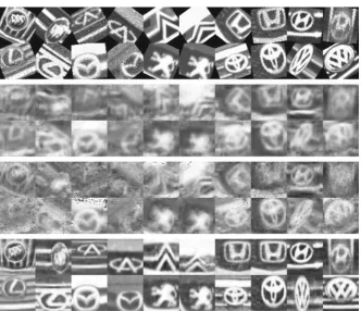
SSIM (O-R) 0.69 0.66 0.64 0.61 0.62

Fig. 9 Occlusion restoration results by the Joint-CNN-Net , Joint-RED-Net and Joint-Cap-Net with the maximum occlusion box of size[30×30]

In contrast, the Joint-Cap-Net has much better performance in terms of accuracy and robustness to image rotations. For instance, when all training and testing images are randomly rotated within an angle range from −60◦ to 60◦, the Joint-Cap-Net achieves an accuracy of 99.93%, while Joint-CNN-Net could only achieve an accu-racy of 89.06%. This is due to the capsules extracting more robust features than the max-pooling in CNNs. The Joint-RED-Net was adapted from the state-of-the-art recognition network VGG and ResNet. This results in a similar recognition when compared with Joint-Cap-Net. In addition, the PSNR and SSIM measures have been greatly improved for the Joint-Cap-Net, when comparing the O-R with O-D.

4.2.3 Occlusion Robustness Evaluation

Table 4 Performance of Joint-CNN-Net, Joint-RED-Net and Joint-Cap-Net on occluded images

Accuracy(%) PSNR (O-D) PSNR (O-R) SSIM (O-D) SSIM (O-R)

Joint-CNN-Net 99.47 25.86 21.48 0.91 0.67

Joint-RED-Net 99.07 31.85 0.95

Joint-Cap-Net 100 22.07 0.66

The bold indicates the best performance in terms of accuracy, PSNR and SSIM

the recovered version of the corresponding test images by Joint-CNN-Net, followed by images restored by Joint-RED-Net and Joint-Cap-Net. As shown in Table4, the recognition results of Joint-CNN-Net, Joint-RED-Net and Joint-Cap-Net are similar, with an accuracy of 99.47%, 99.07% and 100%, respectively.

With respect to image restoration, Joint-CNN-Net and Joint-RED-Net have certain recovery abilities, at least the white boxes become slightly transparent. Joint-RED-Net recovers the noise, and the recovered images have undesirable effects. In contrast, the Joint-Cap-Net has removed completely the blocking effects and it is difficult to detect that anything has been occluded. The PSNR and SSIM of the recovered images have decreased in the Joint-CNN-Net and Joint-Cap-Net with respect to degradation. This can be explained with the fact that the occlusion changes only a limited small area of the image, while the images recovered by the Joint-CNN-Net and Joint-Cap-Net change the value on every pixel. The occlusion effects have been removed and the visual qualities have been improved by both frameworks, especially by the Joint-Cap-Net. The Joint-RED-Net has high PSNR and SSIM values while conveying a low visual quality.

4.2.4 Mixed-Degradation Robustness

In the previous evaluations, we notice that the Joint-Cap-Net always tends to denoise and rotate the angles automatically even when the networks were trained on other tasks. In order to validate the performance of the proposed framework under very challenging conditions, different image degradations are combined together in the training and testing stages. The results are presented in Fig.10. The first two rows show the combined degradation due to a zero-mean Gaussian noise (variance equal to 0.1), rotation (with a random angle from−60◦to 60◦) and occlusion (with a square white box with a random size from 0 to 30 pixels). The following rows of Fig.10

represent the recovered images from Joint-CNN-Net, Joint-RED-Net and Joint-Cap-Net, respectively.

Clearly, Joint-CNN-Net and Joint-RED-Net cannot deal with rotation and occlu-sion. This makes the recovered images difficult to distinguish by a human observer. On the contrary, the Joint-Cap-Net successfully recovers the image after the combined degradation of rotation, occlusion and noise.

Fig. 10 The restoration result of the Joint-CNN-Net, Joint-RED-Net and Joint-Cap-Net with combined Gaussian noise, rotation and occlusion

Table 5 Performance of the Joint-CNN-Net, Joint-RED-Net and Joint-Cap-Net on combined degradations

Accuracy(%) PSNR (O-D) PSNR (O-R) SSIM (O-D) SSIM (O-R)

Joint-CNN-Net 65.42 7.55 12.82 0.05 0.09

Joint-RED-Net 90.73 12.33 0.06

Joint-Cap-Net 91.39 17.26 0.43

The bold indicates the best performance in terms of accuracy, PSNR and SSIM

5 Summary

joint frameworks based on CNNs (Joint-CNN-Net and Joint-RED-Net) achieve good results on noisy images but have limitations on image rotation and occlusion. The joint capsule network, called Joint-Caps-Net, achieves better results than the Joint-CNN-Net and Joint-RED-Joint-CNN-Net in terms of recognition accuracy and restoration measures. The key to the success of learning capsules is due to a more efficient routing process compared to the pooling process in CNNs. Finally, the proposed joint frameworks are not restricted to the considered application but could be applied to other image recognition/restoration tasks and could use different inner network architectures.

Acknowledgements This work has been partially supported by the “SETA project: An open, sustainable, ubiquitous data and service for efficient, effective, safe, resilient mobility in metropolitan areas” funded from the European Union’s Horizon 2020 research and innovation program under Grant Agreement No. 688082. Nidhal C. Bouaynaya was funded by a US National Science Foundation (NSF) grant under Award Number DUE-1610911. This work was jointly supported by the Research Funds of Chongqing Science and Technology Commission (Grant No. cstc2017jcyjAX0293).

Open Access This article is distributed under the terms of the Creative Commons Attribution 4.0 Interna-tional License (http://creativecommons.org/licenses/by/4.0/), which permits unrestricted use, distribution, and reproduction in any medium, provided you give appropriate credit to the original author(s) and the source, provide a link to the Creative Commons license, and indicate if changes were made.

References

1. G. Chen, Y. Li, S.N. Srihari, Joint visual denoising and classification using deep learning, inProceedings of IEEE International Conference on Image Processing, Phoenix, AZ, USA(2016), pp. 3673–3677 2. R. Chen, M.A. Jalal, L. Mihaylova, R. Moore, Learning capsules for vehicle logo recognition, in

Proceedings of the International Conference on Information Fusion, Cambridge, UK(2018) 3. K. Dabov, A. Foi, V. Katkovnik, K. Egiazarian, Image denoising by sparse 3-D transform-domain

collaborative filtering. IEEE Trans. Image Process.16(8), 2080–2095 (2007)

4. A. Daneshmand, F. Facchinei, V. Kungurtsev, G. Scutari, Flexible selective parallel algorithms for big data optimization, inProceedings of the 48th Asilomar Conference on Signals, Systems and Computers

(2014), pp. 3–7

5. A. Daneshmand, F. Facchinei, V. Kungurtsev, G. Scutari, Hybrid random/deterministic parallel algo-rithms for convex and nonconvex big data optimization. IEEE Trans. Signal Process.63(15), 3914–3929 (2015)

6. I. Dassios, K. Fountoulakis, J. Gondzio, A second-order method for compressed sensing problems with coherent and redundant dictionaries. arXiv preprint:arXiv:1405.4146(2014)

7. I.K. Dassios, K. Fountoulakis, J. Gondzio, A preconditioner for a primal-dual newton conjugate gra-dient method for compressed sensing problems. SIAM J. Sci. Comput.37(6), A2783–A2812 (2015) 8. J. Deng, W. Dong, R. Socher, L.J. Li, K. Li, L. Fei-Fei, Imagenet: a large-scale hierarchical image

database, inProceedings of IEEE Conference on Computer Vision and Pattern Recognition, Miami, FL, USA(2009), pp. 248–255

9. C. Dong, C.C. Loy, K. He, X. Tang, Image super-resolution using deep convolutional networks. IEEE Trans. Pattern Anal. Mach. Intell.38(2), 295–307 (2016)

10. D. Glasner, S. Bagon, M. Irani, Super-resolution from a single image, inProceedings of the IEEE International Conference on Computer Vision, Kyoto, Japan(2009), pp. 349–356

11. K. He, X. Zhang, S. Ren, J. Sun, Deep residual learning for image recognition, inProceedings of the IEEE Conference on Computer Vision and Pattern Recognition, Las Vegas, NV, USA(2016), pp. 770–778

13. M. Jaderberg, K. Simonyan, A. Zisserman, et al., Spatial transformer networks, inProceedings of the Advances in Neural Information Processing Systems, Montréal, Quebec, Canada(2015), pp. 2017– 2025

14. K.I. Kim, Y. Kwon, Single-image super-resolution using sparse regression and natural image prior. IEEE Trans. Pattern Anal. Mach. Intell.32(6), 1127–1133 (2010)

15. A. Krizhevsky, I. Sutskever, G.E. Hinton, ImageNet classification with deep convolutional neural networks, inProceedings of the 25th International Conference on Neural Information Processing Systems, Lake Tahoe, Nevada, USA(2012), pp. 1097–1105

16. Y. Lecun, L. Bottou, Y. Bengio, P. Haffner, Gradient-based learning applied to document recognition. Proc. IEEE86(11), 2278–2324 (1998)

17. D.G. Lowe, Distinctive image features from scale-invariant keypoints. Int. J. Comput. Vis.60(2), 91–110 (2004)

18. X. Mao, C. Shen, Y.B. Yang, Image restoration using very deep convolutional encoder-decoder networks with symmetric skip connections, in Proceedings of the Advances in Neural Information Processing Systems, Barcelona, Spain (2016), pp. 1802–2810

19. T. Ni, J. Zhai, A matrix-free smoothing algorithm for large-scale support vector machines. Inf. Sci.

358–359, 29–43 (2016)

20. L.I. Rudin, S. Osher, E. Fatemi, Nonlinear total variation based noise removal algorithms. Phys. D: Nonlinear Phenom.60(1–4), 259–268 (1992)

21. S. Sabour, N. Frosst, G.E. Hinton, Dynamic routing between capsules, inProceedings of the Advances in Neural Information Processing Systems, Long Beach, CA, USA(2017), pp. 3859–3869

22. D. Scherer, A. Müller, S. Behnke, Evaluation of pooling operations in convolutional architectures for object recognition, inProceedings of International Conference on Artificial Neural Networks, Thessaloniki, Greece(2010), pp. 92–101

23. H.R. Sheikh, M.F. Sabir, A.C. Bovik, A statistical evaluation of recent full reference image quality assessment algorithms. IEEE Trans. Image Process.15(11), 3440–3451 (2006)

24. K. Simonyan, A. Zisserman, Very deep convolutional networks for large-scale image recognition, inProceedings of the International Conference on Learning Representations, San Diego, CA, USA

(2015), pp. 1–14

25. N. Srivastava, G. Hinton, A. Krizhevsky, I. Sutskever, R. Salakhutdinov, Dropout: a simple way to prevent neural networks from overfitting. J. Mach. Learn. Res.15(1), 1929–1958 (2014)

26. C. Szegedy, W. Liu, Y. Jia, P. Sermanet, S. Reed, D. Anguelov, D. Erhan, V. Vanhoucke, A. Rabinovich, et al., Going deeper with convolutions, inProceedings of the IEEE Conference on Computer Vision and Pattern Recognition, Boston, MA, USA(2015), pp. 1–9

27. R. Timofte, V. De, L. Van Gool, Anchored neighborhood regression for fast example-based super-resolution, inProceedings of the IEEE International Conference on Computer Vision, Sydney, NSW, Australia(2013), pp. 1920–1927

28. R. Wang, D. Tao, Recent progress in image deblurring. CoRRabs/1409.6838(2014).arxiv:1409.6838

29. Z. Wang, A.C. Bovik, H.R. Sheikh, E.P. Simoncelli, Image quality assessment: from error visibility to structural similarity. IEEE Trans. Image Process.13(4), 600–612 (2004)

30. J. Yang, Z. Lin, S. Cohen, Fast image super-resolution based on in-place example regression, in

Proceedings of the IEEE Conference on Computer Vision and Pattern Recognition(2013), pp. 1059– 1066

31. M.D. Zeiler, R. Fergus, Visualizing and understanding convolutional networks, inProceedings of the European Conference on Computer Vision, Zurich, Switzerland(2014), pp. 818–833

32. H. Zhu, K.V. Yuen, L. Mihaylova, H. Leung, Overview of environment perception for intelligent vehicles. IEEE Trans. Intell. Transp. Syst.18(10), 2584–2601 (2017)