Generalized linear time series regression

City, University of London Institutional Repository

Citation

:

Mammen, E., Nielsen, J. P. & Fitzenberger, B. (2011). Generalized linear time

series regression. Biometrika, 98(4), pp. 1007-1014. doi: 10.1093/biomet/asr044

This is the published version of the paper.

This version of the publication may differ from the final published

version.

Permanent repository link:

http://openaccess.city.ac.uk/18250/

Link to published version

:

http://dx.doi.org/10.1093/biomet/asr044

Copyright and reuse:

City Research Online aims to make research

outputs of City, University of London available to a wider audience.

Copyright and Moral Rights remain with the author(s) and/or copyright

holders. URLs from City Research Online may be freely distributed and

linked to.

City Research Online:

http://openaccess.city.ac.uk/

[email protected]

C

2011 Biometrika Trust Advance Access publication 13 October 2011

Printed in Great Britain

Generalized linear time series regression

B

ENNO MAMMEN

Department of Economics, University of Mannheim, 68131 Mannheim, Germany [email protected]

JENS PERCH NIELSEN

Cass Business School, City University, 106 Bunhill Row, London EC1Y 8TZ, U.K. [email protected]

AND

BERND FITZENBERGER

Department of Applied Econometrics, Albert-Ludwigs-University, 79085 Freiburg, Germany [email protected]

SUMMARY

We consider a cross-section model that contains an individual component, a deterministic time trend and an unobserved latent common time series component. We show the following oracle property: the parameters of the latent time series and the parameters of the deterministic time trend can be estimated with the same asymptotic accuracy as if the parameters of the individual component were known. We consider this model in two settings: least squares fits of linear specifications of the individual component and the parameters of the deterministic time trend and, more generally, quasilikelihood estimation in a generalized linear time series model.

Some key words: Cross-section; Generalized linear time series model; Latent time series; Linear model.

1. INTRODUCTION

Often time series data do not directly lend themselves to a classical analysis, because the series of interest is unobserved. In econometrics, one finds recent extensions of classical panel data models where calendar effects are modelled as genuine time series to allow future forecasts. See, for example, the recent study ofLinton et al.(2009), which gives a review of panel data in this particular context, adds a latent time series to a standard nonparametric regression problem, and shows that under certain assumptions one can analyse the estimated latent time series as if it had been fully observed from the beginning. In this paper, we consider a broad class of parametric models with latent time series and we show the analogous oracle property. One motivation for our analysis comes from an econometric labour market application with an additional identifiability issue arising in demographical age-period-cohort models. In demography, the principle of a latent time series has long been used in mortality estimation and pre-diction, in particular since the appearance ofLee & Carter(1992) andCarter & Lee(1992), which first consider the in-sample mortality model in two steps. After the in-sample parameters have been estimated, the estimated calendar effect is redefined into a time series and is analysed as such. In this paper, we prove that under certain regularity assumptions this procedure is valid also when the latent time series is incorporated into the model from the outset. While Lee & Carter(1992) andCarter & Lee(1992) only consider calendar and age effects on mortality, recent studies also model cohort effects; see, for example,

1008

E

M

, J

P

N

B

F

cohort year and age. The forecasting issue arises from the fact that the forecast can be poorly specified even when in-sample parameters are fully identified.Kuang et al.(2008a,2008b) address these two prob-lems. In this paper, we consider one important additive version of the age-period-cohort model and we show that one can estimate the calendar effect and forecast it as if it were fully known from the begin-ning (Fitzenberger et al.,2001;Fitzenberger & Wunderlich,2002). For some related nonparametric mod-els, seePark et al. (2009) and Linton et al.(2009). While the full model formulation approach has for some time been used in demographics and actuarial science (Lee & Miller,2001;Renshaw & Haberman,

2003a,2003b;Wong-Fupuy & Haberman,2004;Li & Chan,2005), it has only recently found its way into econometrics and empirical finance (Fengler et al.,2007;Park et al.,2009).

2. ESTIMATION IN A LINEAR TIME SERIES MODEL

In this section, we consider a linear time series cross-section model

Yi t=Xi tTβ+(Z

T

i tθ)(R

T

tγ+ηt)+εi t (t=1, . . . ,T; i=1, . . . ,I). (1)

For simplicity of notation, we assume that the upper limit I of individualsi does not depend on timet. We observe the response Yi t and the random covariables Xi t andZi t. The vectors Rt are deterministic

covariates to model the time trend. The processηt is a common unobserved latent time series. We assume

that the first elements ofZi tandθare equal to unity. This linear model is related to the one factor models

ofBai & Ng(2006) andBai(2009).

We consider estimation of the time trend parameterγ and parametric fits for the time series structure of the processηt. The parameterβ is the regression parameter. We propose to estimateβ andγ by least

squares. Our main result is to show the following oracle property. Asymptotically the least squares esti-mator ofγ and estimators of the time series parameters ofηtwork as well as if the nuisance parameterβ

were known. We putμt=RtTγ +ηt,νt=θμtand we consider the following estimator ofβand fit ofμt,

(β,ˆ νˆt) = arg min

β,νt

i=1,...,I;t=1,...,T

(Yi t−Xi tTβ−Z

T

i tνt)2,

(θ,ˆ μˆt) = arg min

θ,μt

i=1,...,I;t=1,...,T

{ZT

i t(νˆt−θμt)}2, (2)

where the second argmin runs over vectorsθwith first element equal to one. The time trend parameterγ is estimated by

ˆ

γ=arg min γ

T

t=1

(μˆt−RtTγ )

2_.

(3)

Fits of the time series model forηt are based on the estimation of its autocovariances

ˆ

ρh=T−1

T−h

t₌1

ˆ

ηtηˆt+h (h0), (4)

withηˆt= ˆμt−Rtγˆ. We assume that:

Assumption1. The variables εi t have conditional mean zero E(εi t|X)=0 and they fulfil the

conditional dependence condition:|E(εi tεj s|X)| (|i− j|,|s−t|),|E(ηuηvεi tεj s|X)| (|i−j|,

|s−t|)(i,j=1, . . . ,I;u, v,s,t=1, . . . ,T) for a function with∞_i,s=0 (i,s) <∞. Here the condi-tioning variableXequals{Xi t,Zi t:i=1, . . . ,I; t=1, . . . ,T}.

Assumption2. The processηt is mean zero and the terms T−1/2

T−h

t=1 Rtηt+h , T−1/2

T−h

t=1 Rt+hηt

(h0) andT−1T

t=1η 2

t and(T−

1T

t=1η 2

t)−

1_{are absolutely bounded in probability.}

Assumption4. The matrixT−1_I−1

i=1,...,I;t=1,...,T X˜i tX˜Ti tconverges in probability to a matrixthat

has full rank. Here,X˜T

i tis the vectorXi tT −ZTi tA−t1I−1

I

j₌1Zj tXTj tandAtis the matrixI−1

I

j₌1Zj tZTj t.

The norms of the elements of matricesI−1I

i₌1Zi tXi tT andI−1

I

i₌1RtXi t(t=1, . . . ,T)are uniformly

bounded in probability. The operator norm of AtandA−t 1is uniformly stochastically bounded.

Assumption5. The covariables Rt may depend on T andT−1

T

t=1RtRtT converges to a full rank

matrix.

Assumption 1 allows dependencies between the errors that are local in time and after a suitable reorder-ing of the individuals also local in i. In applications the reordering may correspond to closeness of the individuals in age, region or other characteristics. Assumption 5 can be achieved by normalizing of Rt

such thatT−1T

t=1RtRtTequals the identity matrix. Assumptions 2 and 4 hold, for example, under

appro-priate stationarity and ergodicity assumptions onXi tandZt.

We compareγˆandρˆhwith the theoretical oracle estimators

˜

γ=

_T

t₌1

RtRTt

₋1 _T

t₌1

Rtμt, ρ˜h=T−1

T−h

t₌1

ηtηt+h.

Our main result is that the difference betweenγˆ andγ˜ and the difference betweenρˆh andρ˜h is

asymp-totically negligible. This means that asympasymp-totically the least squares estimator ofγ and the estimators of the time series parameters ofηt work as well as if the nuisance parameterβ were known. These oracle

properties are stated in the following theorem.

THEOREM1. Under Assumptions1–5,γˆ= ˜γ+oP(T−1/2)andρˆh= ˜ρh+oP(T−1/2), for h0.

The basic argument in the proof of this theorem is to show thatμˆt−μt is asymptotically equivalent

to a weighted average of the error variablesεi t. In the calculation of the least squares estimator ofγ and

of the empirical autocovariances, this term is averaged such that it does not contribute to any first order differences for these estimators and one gets the asymptotic equivalences stated in Theorem1. Our model contains as a special caseZT

i tθ≡1. Then the theorem holds without the assumptionT =o(I2)and it is only

required that I,T → ∞. In the general model the additional requirementT =o(I2_{)is needed to control} the rate ofθˆ−θ.

Example1. We use German labour market data, from a 2% random sample of employees subject to

social security, grouped by year and age for the time period 1980–2004. Fitzenberger et al.(2001) and

Fitzenberger & Wunderlich(2002) used earlier versions of these data. The data also involve information about receipt of unemployment benefits. We analyse annual observations of log median real wages, deflated by the consumer price index, for full-time working males with a completed vocational training degree who work full-time. We measure the age-year group specific unemployment rate by the share of benefit recip-ients. We model log wages as a function of age, cohort and year effects as well as the unemployment rate byVi t=αi+ξt+κt−i+Ui tβ+ei t withVi t log median wages,Ui t unemployment rate,i age,t time,

t−icohort. Here,αi,κt−iandβare parameters,ξtis a time series. The aim is inference on the dynamics

ofξt. Note the identification problem arising from the linear relationship between age, cohort and year.

Therefore, we focus on the second differencesYi t=Vi+1,t+2−Vi,t+1−Vi+1,t+1+Vi t,Xi t=Ui+1,t+2−

Ui,t+1−Ui+1,t+1+Ui t,εi t=ei+1,t+2−ei,t+1−ei+1,t+1+ei t andμt=ξt+2−2ξt+1+ξt. For these

sec-ond differences, the parametersαiandκt−icancel and

Yi t=XTi tβ+μt+εi t. (5)

This is an example of model (1). Analogously, we could take the second order differencesYi t=Vi₊2_,t₊1−

Vi₊1_,t−Vi₊1_,t₊1+Vi t to eliminateξt andρt₋i, orYi t=Vi_,t₊1−Vi_,t−Vi₊1_,t₊1+Vi₊1_,t to eliminateξt

1010

E

M

, J

P

N

B

F

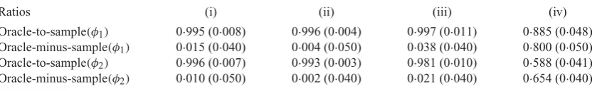
Table 1.Ratios of mean squared differences for the oracle estimator and sample estimator in scenarios(i)–

(iv). Monte Carlo standard deviation is in parentheses and the calculation is based on the delta method

Ratios (i) (ii) (iii) (iv)

Oracle-to-sample(φ1) 0·995 (0·008) 0·996 (0·004) 0·997 (0·011) 0·885 (0·048)

Oracle-minus-sample(φ1) 0·015 (0·040) 0·004 (0·050) 0·038 (0·040) 0·800 (0·050)

Oracle-to-sample(φ2) 0·996 (0·007) 0·993 (0·003) 0·981 (0·010) 0·588 (0·041)

Oracle-minus-sample(φ2) 0·010 (0·050) 0·002 (0·040) 0·021 (0·040) 0·654 (0·040)

Our proposal is to first treatμtas a parameter and to estimateμtandβin equation (5) by least squares;

we estimate heteroscedasticity robust standard errors. The coefficient of the unemployment rateβis esti-mated as 0·097 (0·042), here and henceforth standard errors in parentheses. This significantly positive effect of unemployment likely reflects an inverse labour demand relationship (Card & Lemieux,2001). Our estimates suggest thatμt is fairly precisely estimated, based on standard errors that are estimated,

here and in the following, as ifμt were known; our theory says that the difference is asymptotically

neg-ligible. Next, we investigate the time series process governingμt. The estimated first and second order

autocorrelations are−0·002 (0·209) and−0·476 (0·209), respectively. A Dickey–Fuller test suggests that

μt is not nonstationary. Estimating an autoregressive process of order 2, i.e.,μt=φ1μt₋1+φ2μt₋2+et,

yieldsφˆ1 = 0·0089 (0·202) andφˆ2 = −0·498 (0·202). We find no autocorrelation in the error termet.

Further detailed analysis suggests that the cumulated process ofμt is stationary.

To illustrate the usefulness of our theory, we simulate data based on an idealized version of our sample data. We hold the unemployment rates fixed and we replicate their values when we increase the sample size. We use the model estimates forβ,φ1andφ2to simulate data. We draw the error terms from a normal distribution with zero mean and a variance corresponding to the estimated sample variance. We simulate 1000 random samples for each scenario. We focus on the estimation ofφ1andφ2. Table1reports the ratio of the mean squared error between the oracle estimators, which assumes knowledge of the true simulatedμt,

and the estimators based on the estimatedμt, which we denote by oracle-to-sample(φ), whereφ∈ {φ1, φ2}, and the ratio between the mean squared difference between the sample estimator and the oracle estimator divided by the mean squared error of the sample estimator, which we denote by oracle-minus-sample(φ). These ratios are defined as: oracle-to-sample(φ)=1000s₌1(φ˜s− ˆφ)2/

1000

s₌1(φˆs− ˆφ)2and

oracle-minus-sample(φ)=1000_s=1(φ˜s− ˆφs)2/

1000

s=1(φˆs− ˆφ)2, wheresdenotes the simulated sample,φˆis the parameter

used to simulate the data, φˆs is the sample estimator in thesth simulated sample andφ˜s is the oracle

estimator. We consider four scenarios: (i) the same sample size as in the data application with I=34 andT =23, (ii)T =100 and I=100, (iii) I=15 andT=23 using only age up to 40, (iv) as in (i) but increasing the standard deviation of the error term in model (1) by a factor 10. For scenario (i), the mean squared error of the oracle estimator forφ1areφ2are 0·995 times and 0·996 times, respectively, as large as the mean squared error for the sample estimator, referring to the oracle-to-sample ratios reported in Table1, i.e., for the original sample type the result in Theorem 1 is strongly supported. Furthermore, the oracle-minus-sample ratio is only 1·5 and 1·0% showing the difference between the two estimators is small. Considering scenarios (ii) and (iii), the oracle-to-sample ratio is nondecreasing in the sample size, subject to the Monte Carlo simulation error, and the oracle-minus-sample ratio falls with the sample size. Considering scenario (iv), the oracle-to-sample ratio falls considerably with a larger variance of the error term. These results show that the theoretical considerations are useful for the sample sizes considered here. Further simulation results show that also for estimating the first order autocorrelation of the cumulated process ofμtwe obtain an oracle-to-sample ratio close to one for scenario (i), even though this is beyond

the scope of our theory.

Example2. Our general model (1), with covariatesZi tand parameterθ, can be used in a labour/health

study, where health outcomes depend upon macroconditions, i.e.,γt andηt, interacting with workplace

conditionsZi t. When there is a lot of overtime in a cyclical boom, stressful jobs may result in worse health

worse.Portrait et al.(2010) provides an example, where the cohort process could be modelled as a time series, as in Example 1.

3. GENERALIZED LINEAR TIME SERIES MODEL

In this section, we introduce our generalization through the link functionG:

Yi t=G{XTi tβ+(Z

T

i tθ)(R

T

tγ+ηt)} +εi t (t=1, . . . ,T; i=1, . . . ,I). (6)

The functionG is a known link function. Again as in§2, we observe the responseYi t and the random

covariablesXi tandZi t. As above, the vectorsRtare deterministic covariates to model the time trend and

we putμt=RTtγ+ηtandνt=θμt.

For the theoretical discussion, we assume that for a weighting functionwthe estimatormˆi t=Xi tTβˆ+

ZT

i tνˆt is defined by Assumption 6.

Assumption6. The estimators are approximate solutions of the score equations

sup

t₌1_,...,T

I−1

I

i₌1

{Yi t−G(mˆi t)}w(mˆi t)

=oP(T−1/2),

I−1T−1

i=1,...,I;t=1,...,T

{Yi t−G(mˆi t)}w(mˆi t)Xi t=oP(T−1/2).

Examples for estimators that fulfil Assumption 6 are quasilikelihood estimators in generalized linear time series models. For a positive function V the quasilikelihood function is defined as Q(τ;y)=

y

τ (s−y)V(s)−1dswhereτ is the expectation ofY, i.e., in our caseτ=G(XTβ+ZTν). The quasilike-lihood estimator satisfies the two equations in Assumption 6 withw(u)=G(u)/V{G(u)}. In particular, the equations hold with the right-hand sides replaced by zero. In the next assumption, we assume that

whas bounded support. This simplifies the asymptotic discussion but allows only truncated versions of quasilikelihood estimation.

Assumption7. The functionsGandware twice differentiable and have a bounded second derivative.

The weight functionwhas bounded support.

Assumption8. It holds that

sup

t=1,...,T

ˆνt−νt =oP(T−1/4), ˆβ−β =oP(T−1/4).

We conjecture that Assumption 7 could be weakened to allow a sequence of weight functions with increasing support or even to allow weight functions with unbounded support. But in both cases, one would need rather technical tail conditions. These theoretical discussions are beyond the scope of this paper. In applications we would propose to use the quasilikelihood estimator that corresponds to a weighting function with unbounded support. Assumption 8 is motivated by Assumption 3. For each parameterνt

one hasI observations. This suggests a rate of orderOp(I−1/2)which is equal tooP(T−1/4)according to

Assumption 3. A formal mathematical theory under which technical Assumption 8 holds is also beyond the scope of this paper.

As in the last section, the time seriesμtand the parameterθis estimated as in (2). The trend parameter

γ is estimated by least squares (3). Again, we consider fits of time series models forηt that are based on

the estimation of its autocovariancesρˆh for h0, see (4). We compareγˆ andρˆh with their theoretical

oracle estimatorsγandρhthat are defined as in the last section. We now state an oracle property for (6).

THEOREM2. Under Assumptions 1–8, it holds that γˆ=γ+oP(T−1/2) and ρˆh=ρh+oP(T−1/2)

1012

E

M

, J

P

N

B

F

Example3. Using (6) one can combine the traditional chain-ladder approach with a well-defined time

series analysis of the calendar effect. Consider the case whereYi tis the number of claims in an insurance

portfolio and whereXT

i tβis the sum of two functions. The first function depends on the underwriting year

i. The second function depends on the development periodt−i, i.e., the time it takes for a claim to develop to the pointtwhere the claim is reported to the insurance company. Without the calendar effects this model exactly amounts to the celebrated chain-ladder model whenGis the exponential link function. For many companies the value of such outstanding liabilities is several times the market value of the company. This illustrates the importance of improving the econometric methodology for this problem. Our model above for the first time gives a way to assess the chain-ladder type of regression estimates along with consistently and well-defined time series effect that can be analysed as a standard time series. For a recent extension of the chain-ladder model allowing for calendar effects seeKuang et al.(2008a,2008b) that derive the nontrivial rules of identification and forecasting in this context.

Example4. Similar to Example 1,Fitzenberger & Wunderlich(2004) investigate age, time and cohort effects in labour force participation by females. This analysis could be implemented by estimating a gen-eralized linear time series model using a probit or logit link function. Estimating the time series of labour force participation of females helps to analyse the contributions in the pay-as-you-go social security system or the need for child care.

4. GENERALIZED TIME SERIES REGRESSION

In this section, we briefly consider our final and most general model:

Yi t=G hβ(Xi t)+gθ(Zi t) (RtTγ+ηt)

+εi t. (7)

The model is as in (6) but with the extension of our introduction of two parametric families of functionals h_βandg_θ. This last model has the Lee–Carter model as a special case and it can, for example, also serve to modify the applications of the models (1) and (6).

The model ofLee & Carter(1992) andCarter & Lee(1992) is a special case of (7). Our more general formulation allows the applied statistician to modify Lee and Carter’s original model. For some recent literature estimating the Lee–Carter parameters based on Poisson regression, seeBrouhns et al.(2002), and seeCairns et al.(2009) for modifications of the Lee–Carter structure that are also contained in our model framework. For recent applications to the financial construction of survivor linked bonds, seeBlake et al.

(2006) andDowd et al.(2006).

ACKNOWLEDGEMENT

We thank two referees, the associate editor, and the editor for very useful comments. The first and the last author acknowledge financial support provided by the Deutsche Forschungsgemeinschaft through the research group Statistical Regularization and Qualitative Constraints. We are grateful to Dirk Antonczyk and Stefanie Sch¨afer for excellent research assistance in compiling the data used in Example 1.

A

ˆ

β−β=

T−1I−1

i=1,...,I,t=1,...,T

Xi tXTi t

₋1

T−1I−1

i=1,...,I,t=1,...,T

Xi tεi t, (A1)

ˆ

νt−νt=I−1A−t1 I

i₌1

Zi tεi t−I−1A−t1 I

i₌1

It can be checked thatE( ˆβ−β2|X)=OP(T−1I−1)and thus ˆβ−β =OP(T−1/2I−1/2). Because of

Assumptions 4 and 5 this implies that

sup

t=1,...,T

νˆt−νt−I−1A−t1 I

i=1

Zi tεi t

=OP(I−1/2T−1/2), (A3)

T−1/2I−1

i=1,...,I,t=1,...,T

RtXi tT(βˆ−β)=OP(I−1/2).

From (2) we get that I_t=1,...,T(νˆt,1− ˆμt)2

i=1,...,I,t=1,...,T{Z

T

i t(νˆt− ˆθμˆt)}2

i=1,...,I,t=1,...,T

{ZT

i t(νˆt−νt)}2. This bound and (A3) can be used to show that θˆ−θ=OP(I−1/2) and T−1

T

t=1

(μˆt−μt)2=OP(I−1). With these expansions, one can approximate the score function that is the

deriva-tives of the left-hand side of (2) with respect toθ andμt. After some algebra one gets that θˆ−θ=

OP(T−1/2+I−1)where the rateI−1is a quadratic approximation error coming from the above bounds of

orderOP(I−1/2)forθˆ−θandμˆt−μt. This bound and the linearized score equation can be used to show

that

ˆ

μt−μt=T−1/2I−1 I

i=1

wi tεi t+OP(δt) (A4)

withwi t=(θTZi t)/(θTAtθ)andδt=(T−1/2I−1/2+I−1)(1+ ˆνt−νt + μt). Forγˆ=γ+oP(T−1/2)

we have to show

T−1/2

T

t=1

Rt(μˆt−μt)=oP(1). (A5)

For the proof of this claim note first that, because of (A4), T−1/2T

t=1Rt(μˆt−μt)=

T−1/2_I−1

i=1,...,I,t=1,...,T Rtwi tεi t+OP(I−1/2). Because of (A1), (A4) and (A5) the right-hand

side of this equation is of orderOP(I−1/2). This shows (A5). Thus,γˆ=γ+oP(T−1/2)is shown.

We now show ρˆh=ρh+oP(T−1/2). We have to show for h0 that T1/2(ρˆh−ρh)=T−1/2

T−h t₌1

{(μˆt−RtTγ )(ˆ μˆt+h−RtT+hγ )ˆ −ηtηt+h} =oP(1). For this claim we will show that

T−1/2

T−h

t=1

ηt₊h(μˆt−RtTγˆ−ηt)=OP(T−1/2+I−1/2), (A6)

T−1/2

T−h

t₌1

ηt(μˆt+h−RTt+hγˆ−ηt+h)=OP(T−1/2+I−1/2), (A7)

T−1/2

T−h

t=1

(μˆt₊h−RtT+hγˆ−ηt₊h)(μˆt−RtTγˆ−ηt)=OP(T−1/2+I−1/2). (A8)

Because of (A4), we have that uniformly fort=1, . . . ,T,μˆt−RtTγˆ −ηt=I−1

I

i=1wi tεi t−RTt(γˆ−

γ )+OP(δt). Using this expansion, it can be easily seen that (A6) and (A7) follow from Assumption 3

andγˆ−γ=OP(T−1/2),T−1/2I−1

T−h

t=1

I

i=1ηtwi tεi t+h=OP(I−1/2T−1/2)andT−1/2I−1

T−h

t=1

I i=1

ηt+hwi tεi t=OP(I−1/2T−1/2). The latter expansions follow from Assumption 1.

For ρˆh=ρh+oP(T−1/2) it remains to check (A8). This can be done by showing that

T−1/2T−h t=1 R

T

t(γˆ−γ )RtT₊h(γˆ−γ )=OP(T−1/2), T−1/2I−1

T−h t=1

I

i=1εi tRtT₊h(γˆ −γ )=OP(I−1/2

T−1/2_{), T}−1/2_I−1T−h t₌1

I

i₌1εi t₊hRtT(γˆ −γ )=OP(I−1/2T−1/2) and T−1/2I−2

T−h t₌1

I i₌1

I j₌1

εi t+hεj t=OP(I−1). These expansions can be shown by using Assumptions 1 and 5.

Proof of Theorem2. By expanding the score functions in Assumption 6 we get stochastic expansions of

ˆ

β−βandνˆt−νtwhere the first terms are weighted modifications of the right-hand side of (A1) or (A2),

1014

E

M

, J

P

N

B

F

andˆνt−νt2are of orderoP(T−1/2), see Assumption 8. The further proof of Theorem2can be carried

out by similar arguments as in the proof of Theorem1.

REFERENCES

BAI, J.(2009). Panel data models with interactive fixed effects.Econometrica77, 1229–79.

BAI, J.&NG, S.(2006). Confidence intervals for diffusion index forecasts and inference for factor-augmented regres-sions.Econometrica74, 1133–50.

BLAKE, D.,CAIRNS, A. J. G.,DOWD, K.&MACMINN, R.(2006). Longevity bonds: financial engineering, valuation and hedging.J. Risk Insur.73, 647–72.

BROUHNS, N.,DENUIT, M.&VERMUNT, J. K.(2002). A Poisson log-bilinear approach to the construction of projected lifetables.Insur. Math. Econ.31, 373–93.

CAIRNS, A. J. G.,BLAKE, D.,DOWD, K.,COUGHLAN, G. D.,EPSTEIN, D.,ONG, A.&BALEVICH, I.(2009). A quan-titative comparison of stochastic mortality models using data from England and Wales and the United States.N. Am. Actuar. J.13, 1–35.

CARD, D.&LEMIEUX, T.(2001). Can falling supply explain the rising return to college for younger men? A cohort-based analysis.Quart. J. Econ.116, 705–46.

CARTER, L. R.&LEE, R. D.(1992). Modelling and forecasting U.S. sex differentials in mortality.Int. J. Forecasting 8, 393–411.

DOWD, K.,BLAKE, D.,CAIRNS, A. J. G.&DAWSON, P.(2006). Survivor swaps.J. Risk Insur.73, 1–17.

FENGLER, M.,H¨ARDLE, W.& MAMMEN, E.(2007). A semiparametric factor model for implied volatility surface dynamics.J. Finan. Economet.5, 189–218.

FITZENBERGER, B.&WUNDERLICH, G.(2004). The changing life cycle pattern in female employment: a comparison of Germany and the UK.Scottish J. Polit. Econ.51, 302–28.

FITZENBERGER, B.&WUNDERLICH, G.(2002). Gender wage differences in West Germany: a cohort analysis.German Econ. Rev.3, 379–414.

FITZENBERGER, B.,HUJER, R.,MCCURDY, T. E.&SCHNABEL, R.(2001). Testing for uniform wage trends in West Germany: a cohort analysis using quantile regressions for censored data.Empirical Econ.26, 41–86.

KUANG, D.,NIELSEN, B.&NIELSEN, J. P.(2008a). Forecasting with the age-period-cohort model and the extended chain-ladder model.Biometrika95, 987–91.

KUANG, D.,NIELSEN, B.&NIELSEN, J. P.(2008b). Identification of the age-period-cohort model and the extended chain-ladder model.Biometrika95, 979–86.

LEE, R. D.&CARTER, L. R.(1992). Modelling and forecasting U.S. mortality.J. Am. Statist. Assoc.87, 659–71.

LEE, R. D.&MILLER, T.(2001). Evaluating the performance of the Lee–Carter method for forecasting mortality.

Demography8, 537–49.

LI, S.&CHAN, W.(2005). Outlier analysis and mortality forecasting: the United Kingdom and Scandinavian countries.

Scand. Actuar. J.3, 187–211.

LINTON, O.,NIELSEN, J. P.&NIELSEN, S. F.(2009). Nonparametric regression with a latent time series.Economet. J. 12, 187–207.

PARK, B., MAMMEN, E., H¨ARDLE, W. & BORAK, S. (2009). Time series modelling with semiparametric factor dynamics.J. Am. Statist. Assoc.104, 284–98.

PORTRAIT, F.,ALESSIE, R.&DEEG, D.(2010). Do early life and contemporaneous macroconditions explain health at older ages? An application to functional limitations of Dutch older individuals.J. Popul. Econ.23, 617–42.

RENSHAW, A. E.&HABERMAN, S.(2003a). On the forecasting of mortality reduction factors.Insur. Math. Econ.2, 379–401.

RENSHAW, A. E.&HABERMAN, S.(2003b). On the forecasting of mortality reduction factors.Appl. Statist.2, 119–37.

WONG-FUPUY, C.&HABERMAN, S.(2004). Projection mortality trends: recent developments in the United Kingdom and the United States.N. Am. Actuar. J.8, 56–83.