Pattern formation in squares and rectangles

      

City, University of London Institutional Repository

Citation

:

Jhugroo, Eric (2007). Pattern formation in squares and rectangles. (Unpublished Doctoral thesis, City University)

This is the published version of the paper.

This version of the publication may differ from the final published

version.

Permanent repository link: http://openaccess.city.ac.uk/18271/

Link to published version

:

Copyright and reuse:

City Research Online aims to make research

outputs of City, University of London available to a wider audience.

Copyright and Moral Rights remain with the author(s) and/or copyright

holders. URLs from City Research Online may be freely distributed and

linked to.

PATTERN FORMATION IN SQUARES

AND RECTANGLES

by

Eric Jhugroo

Thesis submitted for the degree of Doctor of

Philosophy

Centre for Mathematical Science

City University

London

Contents

1 Introduction 7

l.1 Background 7

1.2 Plan of Study 10

2 Pattern Formation in Squares 12

2.1 Introduction... 12

2.2 Formulation of the problem 14

2.3 Analysis of the periodic problem. 15

2.3.1 Linear solution . . . 15

2.3.2 Weakly nonlinear solution 16

2.4 Linear solution of the rigid problem 20

2.4.1 Numerical scheme. 21

2.4.2 Accuracy . . . 26

2.4.3 Results... 27

2.4.4 . Comparison with the periodic problem 30

2.5 Weakly nonlinear analysis of the quasi-periodic problem. 31

2.6 Nonlinear solution of the time dependent rigid problem 40

2.6.1 Numerical scheme. . . . 40

2.6.2 Accuracy and validation . . . 42

2.6.3 Results... . . . 43

2.7 Nonlinear solution of the steady-state rigid problem 47

2.7.1 Numerical scheme. 47

2.7.2 Accuracy

2.7.3 Results.

2.8 Discussion . . . .

51

51

3 Pattern Formation in Large Squares 3.1 Introduction . . . .

3.2 Formulation of the problem 3.3 Core expansion . . . . . 3.4 Corner regions . . . . 3.5 Fourier transform theory 3.6 Linear Solution . . .

3.6.1 Solution method 3.6.2 Results . . . .

3.6.3 Comparison with numerical results 3.7 Nonlinear solution .,

3.7.1 Solution method 3.7.2 Results.

3.8 Wall regions 3.9 Discussion . . .

4 Convection Patterns in Rectangles 4.1 Introduction . . . . 4.2 Formulation of the problem 4.3 Results for aspect ratio 0.75

4.3.1 Linear solution ..

4.3.2 Nonlinear time-dependent solutions 4.3.3 Nonlinear steady-state solutions 4.4 Results for aspect ratio 0.5 .

4.5 Discussion... . . 5 Pattern Formation in Large Rectangles

5.1 Introduction... . . . 5.2 Formulation of the problem 5.3 Theory . . . . 5.4 Linear solution .. .

5.4.1 Solution method 5.4.2 Results . . . .

5.4.3 Comparison with numerical results

126

126 · 127 · 129 · 131 · 132 · 135 · 135 · 137 · 137 · 139 · 140 · 141 · 141 · 145 157

· 157 · 158 · 158 · 158 · 161 · 162 166 · 167 235

5.5 Nonlinear solution ... · 243

5.5.1 Solution Method · 243

5.5.2 Results. · 244

5.6 Discussion . . . · 246

Acknowledgements

I would like to express my thanks to Professor Peter Daniels for his guidance and support throughout this research and the preparation of this thesis. I would also like to thank my wife Jay and my sister Emilie for all their help and encouragement. Finally, I would like to thank everyone in the School of Engineering and Mathematical Sciences who has helped me during my period at City University.

Declaration

Abstract

This thesis considers pattern formation governed by the two dimensional Swift-Hohenberg equation in square and rectangular domains.

For the square, the dependence of the solution on the size of the square relative to the characteristic wavelength of the pattern is investigated for pe-riodic, non-periodic (rigid) and quasi-periodic boundary conditions. Linear and weakly nonlinear analysis is used together with numerical computation to identify the bifurcation structure of steady-state solutions and to track their nonlinear development as a function of the control parameter. Non-linear solutions arising from secondary bifurcations and fold bifurcations are also found. Time-dependent computations are also carried out in order to investigate stability, and to find certain nonlinear steady states.

The structure of solutions in the limit where the size of the square is much larger than the characteristic wavelength of the pattern is investigated using asymptotic methods.

For the rectangle, the dependence of the solution on the size of the rectan-gle relative to the characteristic wavelength of the pattern is investigated for non-periodic (rigid) boundary conditions. Most results are obtained for two aspect ratios, 0.75 and 0.5. Linear analysis is used together with numerical computations to identify the bifurcation structure of steady-state solutions and to track their nonlinear development. Nonlinear solutions arising from secondary bifurcations and fold bifurcations are also found, again making use of time-dependent calculations where necessary.

Finally, the structure of solutions in the limit where the size of the rect-angle is much larger than the characteristic wavelength of the pattern is investigated using asymptotic methods.

Chapter

1

Introduction

1.1

Background

Pattern formation through transition from a homogeneous or structureless state to a more complex state is a common occurrence in nature with well known examples occurring in fluid dynamics, chemical reactions and biolog-ical systems (see for example Cross and Hohenberg 1993). In laboratory ex-periments designed to understand such transitions, for example in Rayleigh-Benard convection and Taylor-Couette flow (see the book by Koschmieder 1993), the container walls have a significant impact on the patterns that are observed not only in small aspect ratio systems but also in large scale systems where the dimensions of the geometry are much greater than the characteristic length scale of the instability.

experiments showing the range of patterns observed in Rayleigh-Benard

con-vection include those in square planform containers by Koschmieder (1966),

those in circular planform containers by Koschmieder (1974) and Croquette,

Mory and Schosseler (1983), those on externally excited systems by Chen

and Whitehead (1968) and Croquette and Schosseler (1982) and those on

pattern dynamics by Croquette (1989).

For square containers, finite roll Galerkin approximations to the linearized

system predict an orthogonal combination of "crossed rolls" at onset

(Ed-wards 1988) whereas experiments in large planforms often reveal diagonal

structures (Koschmieder 1966). A possible reason for this discrepancy as

pointed out by Edwards (1988) is that Galerkin representations based on

finite roll approximations parallel and perpendicular to the sides of the

con-tainer are unlikely to be able to predict diagonal roll structures unless a large

number of modes is used and this is generally not possible for large three

di-mensional domains (Arter and Newell 1988). This is a major drawback to

the use of Galerkin methods because the preferred modes at onset generally

do involve diagonal structures.

A better approach may be to use finite-difference or finite-element

meth-ods where no assumptions of the underlying structure of the eigenfunctions

are involved. Even so one of the difficulties still encountered in such studies

is the large computing power needed to solve even the linearized system for

three dimensional domains large enough to contain more than just a few rolls.

This led Greenside and Coughran (1984) to undertake a numerical study of

the simpler Swift-Hohenberg system, a two dimensional relaxational model

(Swift and Hohenberg 1977) designed to contain many of the ingredients of

the Boussinesq system. This has the non dimensional form

au

- = cU - (1

+

\72 }2U - u3

at

'

(1.1 )

where \72 = ~

+ ~,

x and yare non-dimensional Cartesian coordinates, : is a control parameter and

u(x,

y, t) is a characteristic property of the system such as the vertical velocity component. at mid-height in a

horizon-tal fluid layer. The control parameter [ is equivalent to the excess of the

Rayleigh number above its critical value for an infinite layer, where

27r. Greenside and Coughran (1984) carried out a time evolution study of (1.1) identifying many interesting patterns in both squares and rectangular domains and because of the relatively simple form of the equation it was possible to compute patterns over a wide range of domain sizes. Other work on the Swift-Hohenberg equation includes that for a rectangular geometry by Greenside, Coughran and Schryer (1982) and for a circular geometry by l'.Iorris, Bodenschatz, Cannell and Ahlers (1993).

1.2

Plan of Study

The main aim of the present work is to find solutions of the two dimensional Swift-Hohenberg equation in square and rectangular domains. In Chapter 2, the problem is formulated for a square domain 0 ~ x ~ L, 0 ~ y ~ L.

Thus there are two non-dimensional parameters, the control parameter c and the parameter L which determines the size of the domain relative to the characteristic wavelength which for an infinite layer is 27f. Unlike the study of Greenside and Coughran (1984) the main aim here is to undertake a bifurcation analysis allowing the underlying structure and symmetries of the system to be identified for a range of values of L and c. The boundary conditions are taken to be

82

1t 81t

'U = - - 0- = 0 on x = 0, Land y

= 0,

L, (1.2) 8q2 8q

where q is the inward normal to the boundary and 8 in a constant parameter. With 0

=

°

the conditions are referred to as periodic because they are then consistent with periodic solutions of (1.1) in an infinite domain. If

0

is non-zero such solutions are excluded and the conditions are then non-periodic; in particular if £5 is infinite 1t and its first derivative vanish on the boundary,

equivalent to realistic rigid lateral boundaries in the Rayleigh-Benard system. l\lost solutions determined here are for the rigid problem but the periodic problem (0

= 0) and quasi-periodic problem

(0 small) are studied in Sections 2.3 and 2.5 respectively using weakly-nonlinear theory to provide some useful analytical insight. In Section 2.4 a thirteen point finite-difference scheme is used to obtain the eigenvalues [ and eigenfunctions 1L of the steady linearized

these steady-state solutions for increasing €. Secondary bifurcations and

nonlinear fold bifurcations are also identified. The results are compared with experimental findings for the Rayleigh-Benard system in Section 2.8.

In Chapter 3 an asymptotic theory is developed for the square domain in the limit as L -+ 00 and the results are compared with those of Chapter 2. The asymptotic theory is based on the analysis of Daniels (2000) but modified to allow for the corners of the square. This leads to significant dif-ferences in the scalings involved for the control parameter and length scales. The main core expansion is considered in Section 3.3 and uses a multiple scale representation of the roll pattern. The core solution must match with solutions in the corners of the square which are considered in Section 3.4. The leading order core solution is constructed using Fourier transform the-ory in Section 3.5 and linear and weakly nonlinear solutions are determined in Sections 3.6 and 3.7 respectively. Section 3.8 discusses further wall regions that are needed near the boundary of the square to adjust the solution to the rigid boundary conditions. The results are discussed in Section 3.9.

In Chapter 4 the results of Chapter 2 are extended to the case of the rectangular domain although here only the rigid problem is considered. The rectangle occupies the domain 0 ~ x ~ L, 0 ~ y ~ M and most results are for two particular aspect ratios, M / L

= 0.75 and M /

L

= 0.5. These are

described in Sections 4.3 and 4.4 respectively. The results are discussed in Section 4.5.

Chapter 5 considers the limit of large rectangular domains where L -+ 00 and M -+ 00. The asymptotic theory of Chapter 3 is modified in Section 5.3 to allow for the rectangular geometry and linear and nonlinear solutions are obtained in Sections 5.4 and 5.5 respectively. The results are discussed and compared with the numerical results of Chapter 4 in Section 5.5.

Chapter

2

Pattern Formation in Squares

2.1

Introduction

This study investigates convection patterns in a square by finding solutions of the two-dimensional Swift-Hohenberg equation subject to various bound-ary conditions. The aim is to gain insight into the nature of patterns at the onset of convection and also in the supercritical nonlinear regime. The Swift-Hohenberg equation (Swift and Hohenberg 1977) is one of several phe-nomenological models (see, for example, Cross and Hohenberg 1993) which provide a simplification of the three-dimensional Rayleigh-B~nard system but have many features in common with the latter.

the square, such solutions allow the four-fold rotational symmetry of the sys-tem to be preserved, and this helped to explain some of the other patterns observed by Stork and Muller {1972}.

These theoretical and experimental studies of the three-dimensional Rayleigh-Benard system were limited to boxes accommodating up to about six rolls. One of the advantages of studying the Swift-Hohenberg equation is that much larger domains can be investigated numerically, as in the st udy by Greenside and Coughran (1984). They used a time-dependent scheme to study nonlinear pattern evolution for the two-dimensional Swift-Hohellberg equation in rectangular domains, including the square, accommodating up to about thirty rolls. This identified a wide range of possible stable states of the system and although a bifurcation analysis was not carried out the relative stability of various nonlinear states was studied using a Lyapunov functional. A numerical study of a more complex two-dimensional system in rectangular domains has been carried out by Manneville (1983).

Theoretical studies of orthogonal roll patterns governed by the Swift-Hohenberg equation in large rectangular domains (that is, where many rolls can be accommodated) have been carried out by Daniels and Weinstein (1996) and Daniels and Lee (1999) using weakly nonlinear theory based on multiple-scale and matched asymptotic expansion techniques. These studies are limited to solutions composed of roll components parallel and perpendic-ular to the sides of the rectangle and do not include the limiting case of a square domain. Similar methods have been used to study patterns governed by the Swift-Hohenberg equation in large closed two-dimensional domains of arbitrary shape by Daniels (2000).

are modified to incorporate a small rigid component. The next two sections consider the nonlinear system with rigid boundary conditions. Solutions are found using a time-dependent scheme in Section 2.6, and a bifurcation analy-sis of nonlinear steady-state solutions is carried out in Section 2.7 by tracking solutions using Newton iteration. Results are obtained for a wide range of sizes of the square. The results are discussed in Section 2.8.

2.2

Formulation of the problem

The Swift-Hohenberg equation is

8u = EU _ (1

+

\72 )2U _ u3

8t

'

(2.1 )

where t is the non-dimensional time, \72 = ~

+

~ where x and yare non-dimensional Cartesian coordinates, E is a control parameter and u(x, y, t) is

a scalar field.

The geometry that we are considering is a square 0 ~ x ~ L, 0 ~ y ~ L with the equivalent of rigid lateral boundaries so that on the boundary U and

its derivative normal to the boundary vanish: 8u

u

=

8q

=

0 on x

=

0, Land y

=

0,

L.

(2.2) Note that here q is used to denote the inward normal direction.

In order to gain analytical insight we shall also consider the case of pe-riodic boundary conditions where u and its second derivative normal to the boundary are equal to zero at the boundary:

82_u

u

= -

= 0 on x = 0, Land y

=

0, L.

8q2 (2.3)

In Section 2.5 we shall consider a combination of the rigid and periodic conditions:

82_{u 8u}

1£ = - -

6-

= 0 on x

=

0, Land y = 0, L, (2.4)

8q

2

8q

2.3

Analysis of the periodic problem

In this section we shall consider the Swift-Hohenberg equation with the pe-riodic boundary conditions (2.3). We first describe the analytical solution of the linear problem and obtain the eigenvalues c at which steady-state linearized solutions exist. We then find the form of weakly nonlinear steady-state solutions near these bifurcation points and examine their stability.

2.3.1

Linear solution

Solutions of the linearized Swift-Hohenberg equation

8u 2

8t =C1£-(1+V2) u, (2.5)

subject to the boundary conditions (2.3) can be expressed in the form

m7rX n7ry

u = eO'tsin s i n

-L L ' (2.6)

where m and n are positive integers. Substitution into (2.5) shows that the growth rate (J is given by

(2.7)

and that steady-state linearized solutions exist for

(2.8)

Since (J

=

C - Cmn, our analysis shows that the trivial solution u = 0 becomes unstable to the mode (m, n) defined by

. m7rX . ?lily

U

=

U mn

==

sm

L

sm

L'

(2.9)

when C

>

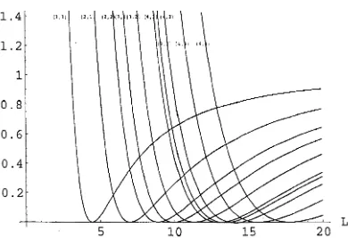
Cmn. Figure 2.1 shows the eigenvalues E'mn plotted as a function of

L.

m n Cmn 1 1 0.044281478 1 2 0.948521881 2 2 4.658144105 1 3 8.689771045 2 3 17.07502964 1 4 32.61930171 3 3 37.28464245 2 4 47.55045122 3 4 78.66988223

Table 2.1: Bifurcation sequence for the case L = 5

Note also that modes (m, n) for which m

=I

n correspond to the existence of repeated eigenvalues C

=

cmn

=

Cnm and thus the possibility of solutions formed from linear combinations of Umn and its orthogonal rotation Unm . A weakly nonlinear analysis is used (below) to identify the actual solutions of the nonlinear system in such cases.

2.3.2 Weakly nonlinear solution

We now investigate solutions of the nonlinear Swift-Hohenberg system (2.1), (2.3) near the bifurcation points (2.8) of the steady state solution. We assume an expansion for U in the form

1 3

'l.t = t2uo

+

tUl

+

t2U2

+ ... ,

(2.10)

\\'here

(2.11)

and 'Ui

=

Ui (x, y, T). Here T is a slow time scale defined by T

= tt

and is included to allow the stability of weakly nonlinear steady-state solutions to be examined. Substitution of

(2.10)

into

(2.1)

and

(2.3)

gives at order t~,

02uo

[image:17.546.221.332.155.333.2]

This is the linearized steady-state system and so the solution is

(2.13) where 1£11111 is the linear eigenfunction defined by (2.9) and a and b are arbi-trary functions of T. Here we allow for the possibility that m =1= n, so that both _{U mn} and _Unm are possible eigenstates; in the case where m = n we may simply take b = O. We do not consider cases where Emn has the same value for different (m, n) combinations, such as (1,7) and (5,5).

At order E, Ul is found to satisfy the same linearized system as Uo:

8

2U I

ttl

= - -

= 0 = 0 at x = 0, L; y = 0, L 8q2

(2.14) and so the solution can be taken to be HI = 0 without loss of generality.

3

At order [2, U2 is found to satisfy the system

8

2112

tt2

= - - =

0 at x

=

0, L; y

=

0, L.

8

q2

(2.15) A consistent solution for U2 requires that the secular terms proportional to

llmn and 'lL_nm on the right-hand side vanish. These can be found by

substi-tuting (2.13) into the right-hand side and expanding the nonlinear term into products of the form sin TIxsin

r

where rand s are integers. After some algebra, it then follows that, from terms proportional to tt_{mn ,} we require

da 9 ₃ 3 ₂

o

= - - a + - a

+ -ab

dT 16 4 ' (2.16)

and, from the terms proportional to 1Lllm , we require

db 9 ₃ 3 ₂

o

= - - b

+

-b

+

-ba .

dT 16 4 (2.17)

First consider the case of a non-repeated eigenvalue (m = n) where we take b = 0 and a satisfies

da 9 3

- =

a - -a.

dT

16

(2.18)

For

t

> 0 we see that there are three steady state solutions

a = as given by as

=

0 and as

=

±~. The local stability of these can be examined by setting

that the trivial solution is unstable for t

> 0, whilst for as

= ±

1

we obtain

(j = -2, showing that the two nonlinear solutions

4 1 . rmrx. n7ry u I"V ±(c c )2sm s m

-3 mn L L ' (2.19)

are stable. The patterns associated with (2.19) for (m, n) = (1,1), (2,2) and (3,3) are shown in Figure 2.2.

Now consider the case of a repeated eigenvalue (m :j n). In this case there are nine steady-state solutions a = as, b = _{bs of} (2.16) and (2.17) consisting of the trivial solution as = _bs = 0 together with:

4 as

=

±-3'

4 as =

± y'2I'

4 as

=

±

v'2f'

bs = 0,

These correspond to supercritical onset solutions for

u

of the form

4 1 m7rX n7ry

u"" ±-(c - c )2sin - - s i n -₃

mn L L '

4 1 n7rX m7ry

u"" ±-(c - c )2sin - s i n - -₃

mn L L '

4 1 m7rx. n7ry . n7rX m7ry

u,..., ± M1(C - cmn)2(sin --sm -L

+

sm - s i n - - ) ,

v21 L L L

(2.20) (2.21) (2.22) (2.23) (2.24) (2.25) (2.26)

4 1 • m7rX n7ry n7rX m7ry

1L ,...,

±

M1(C - Cmll) 2 (sm --sin - - sin - s i n - - ) . (2.27)

v21 L L L L

We can test the local stability of the solutions (2.20)-(2.23) by setting a = as

+

;lear, b

=

b_s

+

Bear and linearizing in A and

f3

in (2.16) and (2.17) to obtain

(2.28)

This yields growth rates ij

=

-2 and ij

=

-~ for each of the solutions (2.20)

and (2.21) which are therefore stable, and growth rates ij

=

-2 and ij = ~

for each of the solutions (2.22) and (2.23), which are therefore unstable. If 11 =

±(foL fo\t2

dxdy)! (2.30) is used as a measure of the amplitude of each solution then for (2.24) and (2.25),

. 1 _! 2 2 ! 2 !

l£ rv "2c2(as +bs )2 = 3(c-cmn

)2

whereas for (2.26) and (2.27)

(2.31 )

(2.32)

so that the solutions (2.24) and (2.25) of larger amplitude

it

are the stable ones.

Finally we consider the nature of the weakly nonlinear patterns associated with the solutions (2.24}-(2.27). We ignore the possibility of changing the sign of 1£ as this will not affect the patterns observed. We shall refer to the

four solutions with the plus signs in (2.24}-(2.27) as 1£1, U2, U3, 1£4 respectively. There are four cases to consider, as follows:

(i) m even,

n

odd

In this case ttl has OE symmetry, i.e it is odd in x about x = ~L and is even in y about y = ~ L. Since 1£2 is obtained from Ul by interchanging x and

y it is just an oithogonal rotation of Ul and has EO symmetry. Solution U3 is unchanged by the transformation x -+ y, y -+ x and is therefore symmetric about the diagonal y =

x.

Its sign is reversed by the transformation L -

x --';

y, y --'; L - x and it is therefore antisymmetric about the other diagonal,

(ii) Tn odd, n even

Interchanging Tn and n in (2.24)-(2.27) is equivalent to swapping Ul and

U2, has no effect on U3 and reverses the sign of 1t4, so the same patterns occur as in (i) except that now Ul has EO symmetry and U2 has OE symmetry. (iii) m. odd, n. odd

In this case Ul and U2 both have EE symmetry. Again U2 is just an orthogonal rotation of Ul. Since Ul and U2 both have EE symmetry, any linear combination of them also has EE symmetry. Thus both U3 and U.j have EE symmetry. In addition, U3 is symmetric about both diagonals y = x,

y = L - x and 114 is antisymmetric about both diagonals. Figure 2.5 and Figure 2.6 show examples with 'In

=

3, 11 = 1 and Tn

=

5, n = 1.

Note that U3 and U4 are those combinations of Ul and U2 which, ignor-ing the sign of the solution for 1t4, possess 4-fold rotational and reflectional symmetry.

(iv) Tn even, n even

In this case ttl and U2 both have

00

symmetry. Again lt2 is just an

orthogonal rotation of Ul. Since Ul and U2 both have

00

symmetry, any linear combination of them also has

00

symmetry. Thus U3 and U4 both have

00

symmetry. In addition, as in (iii), U3 is symmetric about both diagonals and U4 is antisymmetric about both diagonals. Figure 2.7 shows an example with m = 4 and n = 2. Again U3 and U4 are those combinations of ttl and U2 which, ignoring the signs of the solutions, possess 4-fold rotational and reflectional symmetry.

2.4 Linear solution of the rigid problem

The linearized steady-state Swift-Hohenberg equation

is now considered with rigid boundary conditions

au

U

= - =

_aq

0 on x

=

0, Land y

=

0, L.

(2.33)

(2.34)

The system (2.33) is homogenous and constitutes an eigenvalue problem for

convection and the corresponding function u(x, y) determines the pattern of convection at onset. Higher eigenvalues E and eigenfunctions u determine the onset and nature of higher modes of convection at a given value of L. In Section 2.4.1 below a numerical scheme is developed to allow the eigenvalues

E and corresponding eigenfunctions u(x, y) to be determined.

2 .4.1

Numerical scheme

We can solve (2.33) with (2.34) numerically by a finite difference approach. Equation (2.33) is discretised on to a uniform grid

x

=

ih for i

=

0, .. Ai + 1,

y

= jk

for j

= O, .. N +

1,

(2.35 ) (2.36) where hand k are the spatial step lengths in x and y respectively and

(M +

l)h = (N

+

1)k = L. We let Ui,j be the numerical approximation to u at grid

point (i, j) so that (2.33) becomes

(2.37) The spatial derivatives on the right-hand side of (2.37) are approximated using a second-order accurate 13-point central difference representation as

follows. We first expand the right-hand side to get

{ u

+

2uxx

+

2uyy

+

2uxxyy

+

Uxxxx + Uyyyy

h,j .

(2.38) To find approximations to each derivative listed in (2.38) we can use Taylor expansions as follows. For a function

f(x)

of one variable, we have

(

I h

2

/I h

3

11/ h4 1/1/ ( )

f x

±

h)

=

f(x)

±

hf (x)

+

2"

f (x)

± '6

f

(1')

+

24

f (x)

+ ....

2.39

I 2 /I

4h

3

/II

2h4

111/ ( )

f(x±2h)

=

f(x)±2hf (x)+2h f (x)±3f (1')+3 f (x)+ .... 2.40

Adding the two expressions in (2.39) and also the two expressions in (2.40) and solving simultaneously for

J"

and

J"",

gives

/' (x)

=

-~[J(x+2h)-16f(x+h)+30f(x)-16f(x-h)+

f(x-2h)]+O(h").

(" (.1') =

~4

[j(X

+

2h) - 4f(x

+

h)

+

6f(x) - 4f(x - h)

+

f(x - 2h)]

+

0(h2). (2.42)

It also follows directly from adding the two expressions in (2.39) that

" 1 2

f (x)

=

_h2 [j(X + h) - 2f(x)

+

f(x - h)]

+

O(h ). (2.43) Formulae (2.43) and (2.42) provide the following second-order accurate ap-proximations to four of the five derivatives of u(x, y) in (2.38):

1 2

{uxxhj= h2(UH1,j-2ui,j+Ui-1,j)+O(h), (2.44) 1

{llyy hj = k2(Ui,j+1 - 2Ui,j

+

ui.j-d

+

0(k2), (2.45)

{Uxxxxh,j = h4 [Ui+2,j - 4UH1,j I

+

611j,j - 4Ui-1.j

+ Ui-2,j]

+ O(h ),

2 (2.46) and similarly

(2.47) Note that for the second derivatives we use (2.43) rather than the more accurate fourth order approximation (2.41) to maintain a consistent level of approximation. It remains to find a second-order accurate numerical approx-imation to the mixed derivative Uxxyy' To do this, we first use the Taylor expansions of u(x

± h,

y

± k)

and u(x

± h,

y =t= k) to give

ll(x + h, y

+

k) + ll(x - h, y - k)

+

u(x

+

h, y - k)

+

ll(x - h, y

+

k) =

( ) ( 2 ,2 ( h

4

:2 ,2 k 4 ) ( )

411 X, Y

+

2 h

uxx

+

I.; llyy )(x, y)

+

6lLxxxx + h k Uxxyy

+

61lyyyy X, Y +0(h6, h4k2, h2k4, k6) (2.48)

An approximation to ll_{xxyy can now be obtained by using (2.41) and (2.42)}

to replace all of the other derivatives in (2.48), maintaining the error at the order of the sixth power of the step length. From this we obtain

1

{UxXYY}i,j = h₂k₂[411i ,j - 2(lli+l,j

+ 1Li-l.j

+

lli,j+1

+

lli,j-d

h4 1.;4

This gives the discretized form of equation (2.37) as

Di,j

=

clLi,j, i

=

1, .. i'd, j

=

1, .. N, (2.50) where

2 2

Di,j = lLi,j + h₂ (lLHI,j - 2Ui,j + Ui-l,j) + k₂ (Ui,j+I - 2Ui,j + l£i,j-d

1

+-[1L'+2 . -_h4 t ,) 41L+l . t ,J

+

61L . -t,} 41L-I . t ,}

+

1£'-2 .j t ,J 1

+ k4 [lLi,j+2 - 4Ui,j+I

+

61Li,j - 41Li,j-I

+

Ui,j-2j 2

+ h₂k_{2 [}41Li,j - 2(lLHl,j + lLi-I,j + lLi,j+1 + lLi,j-I)

+lLHI,j+l

+

lLi-I,j-1

+

lLHI,j-I

+

lLi-I,j+d. (2.51)

The equations (2.50) apply at all internal points of the grid; this requires evaluation of lLi,j at fictitious points outside the grid where i

=

-1, i

=

M +2, j

=

-1 and j

=

N +2. This is done by using the boundary conditions ~~

=

0 on

x

= 0, Land y = 0, L which in discretised form become

lL-I,j = UI,j, Ui,N+2 = 1Li,N'

(2.52) The values of lLi,j in (2.50) on the boundary are replaced using the condition

'/.l

=

0 on x

=

0, Land y

=

0, L which gives

'/.lO,j

=

lL!vf+I,j

=

lLi,O = Ui,N+l

=

O. (2.53) Since Di,j is a linear function of the Ui,j'S, equation (2.50) can now be expressed in the matrix form

All

= ell, (2.54)

points:

1LM,1

Ul,2

U=

UM,2 (2.55)

Hl,N

HAI,N

and the

NAlxNM

matrix

A

is given by

D

B

C

0 0 0 0 0

B D B C 0 0 0 0

C

B D B

C

0 0 0

0

0 0

A=

C

0 0 (2.56)

D B C 0

0

C

B

D

B

C

0 0 0 C B D B

where

a.j

+

al

+

a5 a2 a4 0 0 0 0 ",

a2 al

+

a5 a2 a4 0 0 0

a.j _{a2 al}

₊

_{a5 a2 a4 0 0}

0 _{0 0}

D=

0 0 _{0 0}

0 0 O· '. 0 0 0

0 _{a2 a4}

0 _{a4 a2 al}

₊

_{a5 a2}

0 0 0 0 0 a4 a2 a4

+

al

+

a5

(2.57)

" _a4

+

_{al a2 a4 0 0 0 0}

a2 al a2 a4 0 0 0

a4 a2 al a2 a4 0 0

0 _{0 0}

D=

0 0 0 0 (2.58)

0 0 O· '. 0 0 0

0 _{a2 a4}

0 _{a4 a2 al a2}

0 0 0 0 0 a4 a2 a4

+

al

a3 ao 0 0 0 0 0

ao a3 ao 0 0 0 0

0 ao a3 ao 0 0 0

0 0 0

B=

0 0 0 0 (2.59)

0 0 0'· . 0 0 0

0 0 0

0 _{ao a3 a6}

c=

o

o

0 0 0 0

o

0

0

0

o

0

o

o

0

o

0

o

0

o

are

M xM

matrices and

4 4 6 6 8

al = 1 - h2 - k2

+ h4

+ k4

+ h

2k2 ' 2 4 4

a2= h2 - h4 - h2k2 ' 2 4 4 a3

=

k2 - k4 - h2k2 '

1

a4

=

h4 '

1

as = k4 '

2 a6 = h2k2 '

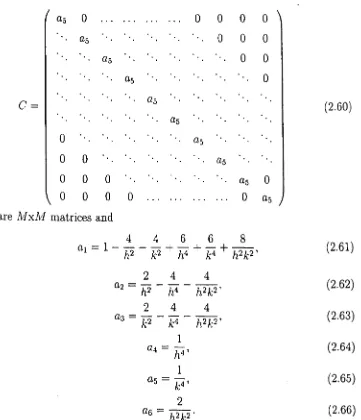
(2.60) (2.61) (2.62) (2.63) (2.64) (2.65) (2.66)

Note that A is a symmetric matrix. The matrix equation (2.54) was solved

using Mathematica, which computes all of the eigenvalues and eigenvectors

by the QR method in which A is first balanced and then transformed into upper Hessenberg form.

2.4.2 Accuracy

[image:27.546.105.466.161.581.2]

Mode h = k = 0.5 h = k = 0.25 h = k = 0.15625 h = k = 0.125 1 1.020972753 1.076166636 1.090222056 1.091083918 2 4.107593799 4.751277379 4.900802877 4.933877698

3 10.08752594 11.82658277 12.24762645 12.346600 4 14.31531158 18.21773996 19.17849635 19.407716

5 14.71007557 18.61901068 19.57322833 19.800523

6 24.58668899 30.58976291 32.11738626 32.487922

7 35.78291717 50.66682575 54.58722708 55.546068

8 45.28573134 57.39985710 60.62084000 61.416953

9 50.52054596 69.01803175 74.04047113 75.284872

10 51.24628780 69.96693461 74.97978581 76.216988

Table 2.2: Leading eigenvalues E for the case L = 5 on various grids

grids are also in reasonable agreement. For higher values of L and higher modes the variation of 1l across the square occurs more rapidly and so it can be expected that larger grids will be required to adequately resolve the solution.

2.4.3 Results

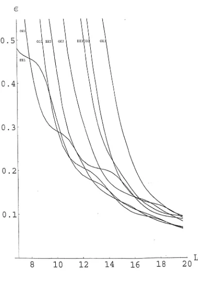
ever-increasing number of modes assume the position of leading eigenmode as L increases, here the most dangerous mode is confined to one of the three branches EEl, OEI and 001. The various branches appear to divide into distinct groups - branches EEl, OEI and 001 constitute the first group and members of the second group include branches EE2, 002 and OE2 (see Figure 2.8). This behaviour is reminiscent of two-dimensional Rayleigh-Benard solutions in finite cavities with rigid lateral walls, where pairs of solutions with odd and even symmetry combine into distinct groups (Drazin 1975, Daniels 1977b).

The leading group of modes consists of solutions with EE symmetry, 00 symmetry and a repeated eigenvalue with OE/EO symmetry. The repeated eigenvalue is associated with two distinct patterns so that this group actually encompasses four patterns covering the various possible symmetry arrange-ments. vVe now discuss in more detail the patterns corresponding to each of the branches EEl, OEI and 001, and how they change as functions of L -unlike the periodic problem, the pattern is not conserved along each branch as L changes.

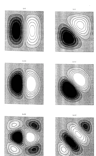
Branch EEl has EE symmetry and at low values of

L

consists of a single-cell or 'one single-cell' solution. Contours of the eigenfunction u associated with this branch at various values of L are shown in Figures 2.10 and 2.11. It is the dominant mode for L

<

8, for 10.1

<

L

<

12.7 and then again when L reaches 18.9; at large L it continues to interweave with branches OEI and 001. The pattern changes in an interesting manner as

L

increases. In the region 8.2

<

L

'<

10.1 (where it is not the dominant mode) it develops four new cells in the corners, sitting at both ends of the diagonals. A further set of four cells is added when 12.7

<

L

< 18.9 and it appears that this process

continues as L increases. A computation for L = 30 (as seen in Figure 2.11) shows that the solution is developing into two sets of cells placed along the diagonals of the square.

defined in Section 3.2. If we assume that 1£1 has EO symmetry then if an

eigenfunction produced by the numerical scheme is denoted by u(x, y) then we can construct 1£1 as

1£1 (x, y) = u(x, y)

+

u(L - x, y). (2.67) Then solution 1l2, which has OE symmetry, is determined as

(2.68) and is just the orthogonal rotation of 1£1. The diagonal mode 113 can now be

determined as

(2.69) and is symmetric about the diagonal y

=

x

and antisymmetric about the diagonal y = L - x. Finally, 1£4 is determined as

(2.70) and is antisymmetric about the diagonal y = x and symmetric about the diagonal y = L - x. Contours of the OE solution 111 and the diagonal

mode 113 at various values of L along branch OE1 are shown in Figures 2.12

and 2.13. At low values of L the solution 1£1 is a 2-cell parallel mode and

113 is a 2-cell diagonal mode, resembling the corresponding solutions of the

periodic problem (Figure 2.3). The branch OE1 modes are dominant when 8.2

<

L

<

10.1, 12.7

<

L

<

14.4 and then again when 16.8

<

L

<

18.9. As

L

increases, the diagonal mode 113 gains additional cells and the simplest way

of interpreting 1£1 is as a superposition of this solution and its orthogonal

rotation (1l1(X, y) = ~(1£3(X, y) +1£4(X, y))). Thus at large L the solution 111 is

effectively a combination of cells placed along each diagonal- any resemblance to a parallel mode no longer exists. At L = 30, the solution 'l.Ll is visually

similar to that of branch EEl at L = 30; the main difference is that whereas branch EEl has EE symmetry and therefore contains an odd number of cells along each diagonal, the OE symmetry of 1£1 implies that it must contain an ('yen number of cells along each diagonal.

of a '4-cell' solution similar to the (2,2) mode of the periodic problem. This branch becomes the dominant mode for 14.4

<

L

<

16.8. Four new cells appear in the corners when L ::::; 14 and at L = 30 the solution consists of a combination of 12 cells placed along each diagonal. In this case the

00

symmetry of the solution implies that there are an even number of cells along each diagonal, like the solution 'I.ll of branch OE1, but the solution here differs in that there is a saddle-point zero of 1£ at the centre of the square, and the cells in the opposite corners are of common sign.

Figures 2.16, 2.17 and 2.18 show contours of u at various values of Lon the branches EE2, EE3 and OE2. There is again an indication that diagonal patterns emerge at large values of

L,

but with dual cells along the diagonals rather then single cells.

2.4.4 Comparison with the periodic problem

The lack of repeated eigenvalues in the rigid case associated with EE or

00

modes is a significant difference from the periodic problem, although many of the 4-fold symmetric patterns found in the rigid case bear a close resemblance to those which occur in the periodic case, especially for low and moderate values of L. Tests of the numerical code for the rigid problem described in Section 4.1 were carried out with different grid sizes to ascertain whether the lack of repeated EE and

00

eigenvalues could be due to the approximations inherent in the numerical scheme. However, these tests showed no evidence of the convergence of such eigenvalues to common values with increasing grid size.

m n Cmn numerical eigenvalue C

1 1 0.044281478 0.0465318900453688

1 2 0.948521881 0.940022406381974

0.940022406434657 2 2 4.658144105 4.61643751306343

1 3 8.689771045 8.53950540848336

8.53950543374084

2 3 17.07502964 16.8243396048629

16.8243396048807

1 4 32.61930171 31.7016479888962

3l.7016479889166

3 3 37.28464245 36.6636113944453

2 4 47.55045122 46.3760140550676

46.3760142292442

3 4 78.66988223 76.7961119894832

[image:32.546.149.394.154.437.2]

76.7961119894886

Table 2.3: Eigenvalues for the periodic problem with L = 5 obtained numer-ically and analytnumer-ically.

formula (2.8) indicates reasonable agreement given that the numerical scheme

is second-order accurate. Moreover, the scheme correctly identifies whether

eigenvalues are repeated to an extremely high level of accuracy.

2.5

Weakly nonlinear analysis of the

quasi-periodic problem

In Section 2.3 an analysis of the periodic problem showed that there are

repeated eigenvalues

_ (m2

₊

_n2_)rr2 2

C = cmn = (1 - £2 ) ,

corresponding to the fact that for

mfn

. mrrx. '1lrry

tL = tLmn

==

8m [Sln

L'

(2.71)

and u = 1tnm are both eigensolutions of the linearized system. If m is odd and

n is even (or vice versa) these correspond to two weakly nonlinear solutions with EO (or OE) symmetry which also combine to produce two solutions with diagonal symmetry. If m and n are both odd (or both even) they corre-spond to two weakly nonlinear solutions with EE (or 00) symmetry which also combine to produce two solutions with 4-fold EE (or 00) symmetry. In the rigid problem, however, repeated eigenvalues are confined to the modes equivalent to (2.72) with EO (or OE) symmetry, and solutions with EE (or OO) symmetry bifurcate at different values of c. Thus, for example, branch OE1 of the rigid problem (Figures 2.12 and 2.13) is a repeated eigenvalue whereas branches EEl, EE2, EE3 and 001 are distinct. In order to gain insight into this qualitative difference between the periodic problem and the rigid problem, it is proposed in this section to study weakly nonlinear solu-tions of the quasi-periodic system

~~

= cu - (1

+

V2}2u - u3, (2.73)

[Pu

au

u

=

0, aq2 - 8 aq = 0 on x

=

O. L; y

=

0, L. (2.74) Note that here q is used to denote the inward normal direction to the bound-ary and fJ is an arbitrary parameter. The periodic problem corresponds to fJ = 0 and the rigid problem corresponds to 8 = 00. Here it will be assumed

that 8 is small so that analytical progress can be made, and the effect of in-troducing a small component of the rigid boundary condition can be gauged. Kote that the system (2.73), (2.74) possesses the same basic symmetry as the individual periodic and rigid problems.

We assume the amplitude for u is of order 8 and pose an expansion of the form

(2.75) as 8 -+ 0, with

(2.76) and, in order to discuss stability, we incorporate a slow time scale T. where

t

=

8-

2T. Substitution into (2.73)' (2.74) gives, at order

8

{Puo

This is just the linearized periodic problem, with solution

(2.78)

where a(T) and b(T) are arbitrary amplitudes, U mn is defined by (2.73) and

Emn by (2.71). Since we are interested specifically in the possibility of re-peated eigenvalues, we shall assume that 'm =I- n. The objective of the anal-ysis is to determine the amplitude equations for a and b by continuing the analysis to higher levels of approximation.

At order 82, lil is found to satisfy

(2.79)

with boundary conditions

UI = 0, a2UI oUo X

= 0,

ox2 ox on (2.80)

HI = 0, a

2_{U1 auo}

x=L,

- - = - - on

ax2 ax (2.81)

HI = 0, a2Ul _ay2 ouo y

= 0,

ay on (2.82)

U1 = 0, 02UI - - = - -auo on y

=

L.

ay2 ay (2.83)

A solvability condition for this system can be derived by introducing an

adjoint function

Uo = CUmn

+

du_{nm ,} (2.84)

where C and d are arbitrary constants. ~Ilultiplication of (2.79) by

uo

and

integration over the square gives

foL foL

uo(l

+

\12)2uldxdy - co

foL foL

uouldxdy =

E'1

foL foL

uouodxdy. (2.85)

Integration by parts on the left-hand side and use of the boundary conditions

(2.80)-(2.83) then gives

l LlL

2 2

lL

auo aIlo auo auo

ul((l

+

\1 ) Uo - E'ouo)dxdy

+

(-8 '£.)Ix=o

+

!:l!:llx=ddy

o 0 0 x vX vI vX

In

L

ailo Olto

auo auo

In

L

In

L

-+

(-8 -8

!y=o

+

-8 -8

!y=ddx

= El

ltolLodx,dy.

However, since Uo satisfies the same linear equation as un, the first term on the left-hand side vanishes and evaluation of the remaining terms using (2.78) and (2.84) gives

Terms proportional to c and d must balance separately on each side, but this just fixes

(2.88)

and does not determine the amplitudes a and b. Note that if 8 is positive, this result indicates that the 'rigid' component of the boundary condition has the effect of raising the critical value of E compared to its value for the

periodic problem. The amplitudes a and b must be found by proceeding to the next order in the expansion, but before doing this it is necessary to find an explicit solution for U1'

Since the solution for Ul is forced by that for Uo, it is possible to write

(2.89)

and

(2.90) \\'here

. m1TX . n1Ty

Umn = Fmn(y)sm

L

+

Fnm(l')sm

L '

(2.91) and, from (2.79), Fmn and Clmn satisfy

1/1/ m27l'2 /I m21T2 ? . n1Ty

Fmn

+

2(1 -

-V

)Fmn

+

[(1 -

---v-)- -

cO,Fmn = Clmnsm

y '

(2.92) From (2.80)-(2.83) the boundary conditions are

Frnn = 0, F _{mn -}/I _ n1T _L (y = 0); Fmn = 0, Fmn /I = (-1) n+1 n1T

L

(y =

L).

(2.93) The solution for Fmn exists provided that Clmn

=

4n21T2 L -3 and is given by

I

n7l' (coshk~n(Y-~L) ?y-L mry )

Fmn=-- 1

+

c o s

-2Lqmn cosh lk~nL L L

2

if n is odd, and

1

F rnn - - - -_ n7r ( sinhk~n(Y 1 - ~L)

+

2y - L cos - -n7rY )

2 Lqrnn sinh lk1~nL L L

2

(2.95)

if n is even, where

(2.96)

and

(2.97)

For a given mode (m, 11.), qmn and k_mn are positive for low values of Land negative for high values of L. For kmn

<

0 the solutions (2.94) and (2.95) generally remain valid with the hyperbolic functions replaced by the corre-sponding trigonometric functions. It is evident however that the theory must be revised to deal with resonant cases for certain discrete negative values of kmn and also in the case qmn = 0 corresponding to the minimum points of the marginal stability curves in Figure 2.1. The expansions (2.75) and (2.76) would need to be modified to treat these special cases but here we focus on general values of m, 11. and L.

Strictly speaking, the solutions (2.94) and (2.95) can also contain an ad-ditional term Asin

T

where A is an arbitrary constant, but this is just equivalent to the fact that Ul can contain an arbitrary multiple of tlQ, corre-sponding to a renormalization of the overall solution. We therefore proceed taking A = 0; .it can be confirmed that if A is non-zero, it does not influence the amplitude equations for a and b determined below. Note that the value of Clmn

+

[lnm confirms the earlier result (2.88) for [1 given by using the

solvability condition. Note also the non-trigonometric form of

Fmn

and the asymmetry in T and y which arises from the influence of the 'rigid' component of the boundary conditions around the square.

At order 62, U2 is found to satisfy

2 2 3

Ouo

(1

+

\l ) U2 - COU2 = Cl UI

+

C2 UO - Uo -

or'

with boundary conditions

02'll2 OUI

- - - -

_ox

on

x=O,

2 -

ox

(2.98)

'U2 = 0,

{J2U2 {JUI

x=L, (2.100)

= on

{Jx 2 {Jx

lt2 = 0, {J2U2

₌

{JU1 on Y = 0, (2.101)

{Jy2 {Jy

1£2 = 0, - - = - -{J2U2 {JUI on Y

=

L. (2.102)

{Jy2 _oy

The solvability condition for this system is found by multiplying (2.98) by

the adjoint function (2.84) and integrating over the square, giving

lo

L

(ouo ~ ~ OU1

I _

x-O

+

OUo ~ ~ 01£1

I

x-L _)d Y

+

1L

(GUo G OUl~

l

y-O

_

+

OUo ~ ~ 01£1

I _

y-L )dr

o ux ux uX uX 0 y uy uy uy

{L {L_

{L {L_

{L {L_ 3

= C1 io io uou1dxdy

+

C2 io io uouodxdy - io io uouodxdy {L {L 01£0

- io io Uo

aT

dxdy. (2.103)

All of the integrals involved in this equation can be calculated from the known

expressions for 1£0, U1 and

uo.

From terms proportional to c, after extensive algebra and for m =1= n, this gives

(2.104) and from terms proportional to d,

1 2 db 1 2 2 9 3 3 2

-L -.-+klb+k2a=-Lc2b-L (-b +-ba)

4 dT 4 64 16 ' (2.105)

where the coefficients on the left-hand side are given by

(2.106)

(2.107)

Here

if m,n are both even or both odd and Omn = 0 if m is even and n is odd (or vice versa),

and

{

mr

2 J

IJ

= I ( ) _ 2Lq",,,(I-kmntanh2kmnL),

rmn-Fmn 0 - ! !

7l1r

(2

k' 2 coth

1

k 2 L)

-2L -L -_q"ul mn -2 mn ,

By introducing the scale transformation

1 k2 = -L2k

4 and a local control parameter f defined by

(2.109)

n odd;

(2.110) n even.

(2.111)

(2.112)

the amplitude equations (2.104), (2.105) can be written in the simpler form

da

=

Ea _ kb -

~a3

_

~ab2

dr 16 4 ' (2.113)

db = fb _ ka -

~b3

-

~ba2

dr 16 4 ' (2.114)

from which the local bifurcation structure and weakly nonlinear development

can now be deduced. We first discuss steady-state solutions a = Qs, b = bs where the left.,.hand sides are set to zero.

First note that if m is even and n is odd (or vice versa) the coefficient k is zero and the equations (2.113), (2.114) are then similar to those discussed in

the periodic problem in Section 2.3 (cf (2.16), (2.17)). This implies that (to within an arbitrary change of sign in u) four steady-state solutions bifurcate from E = 0, two of which are pure EO and OE modes (where either a:; = 0 or bs = 0) and two of which are the diagonal combinations of these modes (where either as

=

b_s or as

=

-b_{s ).} Thus inclusion of the 'rigid' component of the boundary condition has no qualitative effect on the nature of the

bifurcation in this case. This is consistent with the fact that in the rigid

linearized problem (Section 2.4) such modes are still associated with repeated

However, if 'm and n are either both odd or both even, the coefficient k is non-zero, being given from (2.106), (2.107) and (2.111) by

32m2

_nh

_r 4

k= ~~~--~~--~~~~--~~--~

12(n2 7[2

+

3m2 7[2 - 212)(m27[2

+

3n27[2 - 212) (2.115) In this case the bifurcation points from the trivial solution as

=

bs

=

0 of (2.113), (2.114) move to separate locations t

= -k

and t

= k

and correspond

to solutions for which as

=

-b_{s and as}

=

b_{s respectively. The full nonlinear} solutions of (2.113) and (2.114) are

4 I

a _s

=

-b

_s

=

± - ( t

_J2I

+

k)2

_'

t>-k

(2.116)

and

t>k

(2.117)

and are equivalent to the 4-fold symmetric EE or 00 solutions, consistent with the occurrence of separate eigenvalues of the linearized rigid problem

in Section 2.4. Solutions of (2.113), (2.114) for which either as =

0

and bs =1= 0 or as =1= 0 and bs = 0, corresponding to a pure mode U nm or U mn , are no longer possible, but are replaced by solutions which develop from a

secondary bifurcation. This can be seen by multiplying (2.113) by bs , (2.114)

by a~ and subtracting to obtain

2 2 3

(as - bs )(k

+

16asbs) = O. (2.118) The solutions for which bs =

±a

s have already been discussed, but there are also solutions for which

16k bs = - - .

3as From (2.113), these are given by

2V2

2 2 1 1

as =

±-3-(t±(t -

36k

)2)2,

(2.119)

(2.120)

(with bs then determined from (2.119)) and exist for t~6Ikl. These four solutions bifurcate from the leading branch of (2.116), (2.117) at t =

61kl

where

lasl

=

Ibsl

=

4(t/3)L

As t increases, however, one pair of solutions

E-+OO and the other pair becomes dominated by the b_s component, with

JasJ

-+

0,

Jb_sJrv

4d

/3

as E-+OO. Thus the pure U_mn and _{U nm} modes emerge on these secondary branches as E-+OO. Note that using the measure (2.30) the overall amplitude of the solutions (2.116), (2.117) is

1 2 2 1

[8

1

iLrv"20(as

+

bs )2

=

V

2i

OE2 , (2.121) whereas the overall amplitude of the secondary solutions (2.119), (2.120) is slightly larger with

(2.122)

Figure 2.19 shows the bifurcation diagram for the case where m = 3,

'/l = 1 and L = 5, in which case k = 0.07244 in (2.113), (2.114). Solutions for

11 on the various branches, constructed from (2.78), are shown in Figure 2.20. The bifurcation diagram will look qualitatively the same for any value of k

since k can be removed from the equations (2.113), (2.114) by a rescaling of [,a,b and T. Negative values of k are just equivalent to changing the sign of one amplitude function relative to the other.

Finally the local stability of these steady-state solutions can be examined

using the method described in Section 2.3 for the periodic problem. Writing a = as

+

AeaT , b

=

b_s

+

BeaT, substituting in (2.113), (2.114) and linearizing in

.4.

and

iJ

yields the growth rates

a

from the equations

_ _ 27 2 3 2 - 3

-(0' - E:

+

16as

+

'4bs )A + (k

+

"2asbs)B = 0, (2.123)

_ _ 27 2 3 2 - 3

-(0' - E

+

16bs

+

'4as )B

+

(k

+

"2asbs)A = O. (2.124)

Substituting the solutions for as and _bs• this shows that only the branch (2.117) or (2.118) which bifurcates first ((2.117) if k

> 0

or (2.118) if k

<

0) is stable, and since the maximum growth rate is given by

2

a

= 7(E -

6JkJ),

(2.125)

this branch loses stability when E reaches the value

61kl.

At

this point the sec-ondary branches given by (2.119), (2.120) bifurcate and these have maximum growth rate

a-

=

_~€

+

(25 {2

+

24k2)~

\vhich remains negative for t >

61kl.

Thus the secondary branches become the st.able steady-state solutions of the system.

2.6

Nonlinear solution of the time dependent

rigid problem

The time dependent form of the Swift-Hohenberg equation is a nonlinear

system in two spat.ial variables and time. This is a non-trivial system and

cannot be solved in general by analytical means. In this section we describe

numerical solutions of the system. We will focus on the discretisation of

the system and the various numerical methods employed, the accuracy and

stability of the numerical schemes that we derive and finally the results that

our scheme produces from various initial conditions.

2.6.1

Numerical

scheme

The simplest approach is to use an explicit forward difference scheme in which

the SWift-Hohenberg equation (2.1) is replaced by the discretised form

'U,

-u·

~,J 1,] _ - . . _{(1+~2)2-} .. _-3

6.t - E1L~,J v U I,J Ui,j' (2.127)

Here Ui,j is the solution at time t

+ 6.t

and position x = ih, y = jk, i = 0, ... M

+

1; j

=

0, ... N

+

1, where hand k are the step lengths in the x and y directions respectively and (M

+

l)h = (N

+

l)k = L; ui,j denotes the corresponding solution at time

t.

The discretisation of the term (1

+

\7 2) 2U is carried out using central differences exactly as in Section 2.4. This yields a scheme with truncation

errors of order h2 and ).;2 in the spatial derivatives and of order 6.1. in the time derivative:

U·· - U·· 2

1,) ~,J

( 1 ) -

(-

2-

+-

)

6.t = c - Ui,j - h_{2 UHl,j -} Ui,j Ui-l,j

2

1

- k

_{2 (Uj,J+l -} 2Ui,j

+

ui,j-d-h4 (UH2,j - 4Ui+l,j

+

6Ui,j - 4Ui-l,j

+

Ui-2,j)

2

- h₂k_{2 [}4Ui,j - 2(UHI,j + Ui-l,j + Ui,j+l + ui,j-d

+UHI,HI

+

Ui-l,j-l + UHI,j-1 + Uj-l,i+d for i

=

1, ... !vI; j = 1, ... N. (2.128) The equation (2.128) is applied at all internal points; this requires evaluation of Ui,j at fictitious points outside the grid where i

=

-1, i = !vI

+

2, j

=

-1 or j

=

N

+

2. This is done by using the boundary conditions ~~

=

0 on x

=

0, Land y

=

0, L which in discretised form become

(2.129) Values of Uj,j in (2.128) on the boundaries are replaced using the condition 11

=

0 on x

=

0, Land y

=

0, L giving

(2.130) Thus (2.128) provides the solution Ui,j at time t

+

6.t at all internal grid points, and Ui,j is zero on the boundaries. In this way the solution can be

computed forwards in time, from a specified initial state

Uj,j = Ui,j at t

=

0, (2.131) Several other numerical schemes were also considered as follows. A

mod-ified Euler scheme (pseudo predictor/corrector) was developed as a possible

means of increasing the time step used in the numerical scheme. The scheme

takes the form

Uj,j = Uj,j

+

6.tf(Ui,j), (2.132) U· . _t,J

=

U· . _t,J

+

6.t (f(u .. ) _{2 t,]}

+

f(u .. )) _t,J

= ~(u

_{2 t,J} . .

+

u· .) _t,]

+

6.tf(u .. ) _I,J (2.133) where f(Ui,j) is the right-hand side of (2.127) and Ui,j is the corrected value

of the solution at time t

+

6.t.

The Dufort-Frankel leapfrog method was also considered with a view to

improving stability. This is a three-time-level scheme but for a fourth-order

equation in two spatial variables is not generally explicit and is therefore