warwick.ac.uk/lib-publications
Manuscript version: Author’s Accepted Manuscript
The version presented in WRAP is the author’s accepted manuscript and may differ from the published version or Version of Record.
Persistent WRAP URL:
http://wrap.warwick.ac.uk/115622
How to cite:
Please refer to published version for the most recent bibliographic citation information. If a published version is known of, the repository item page linked to above, will contain details on accessing it.
Copyright and reuse:
The Warwick Research Archive Portal (WRAP) makes this work by researchers of the University of Warwick available open access under the following conditions.
Copyright © and all moral rights to the version of the paper presented here belong to the individual author(s) and/or other copyright owners. To the extent reasonable and
practicable the material made available in WRAP has been checked for eligibility before being made available.
Copies of full items can be used for personal research or study, educational, or not-for-profit purposes without prior permission or charge. Provided that the authors, title and full
bibliographic details are credited, a hyperlink and/or URL is given for the original metadata page and the content is not changed in any way.
Publisher’s statement:
Please refer to the repository item page, publisher’s statement section, for further information.
Authors are encouraged to submit new papers to INFORMS journals by means of a style file template, which includes the journal title. However, use of a template does not certify that the paper has been accepted for publication in the named jour-nal. INFORMS journal templates are for the exclusive purpose of submitting to an INFORMS journal and should not be used to distribute the papers in print or online or to submit the papers to another publication.
Online Algorithms for Multi-Level Aggregation
Marcin Bienkowski
Institute of Computer Science, University of Wroc law, Poland
Martin B¨ohm
CSLog, Universit¨at Bremen, Germany and Computer Science Institute, Charles University, Czech Republic
Jaroslaw Byrka
Institute of Computer Science, University of Wroc law, Poland
Marek Chrobak
Department of Computer Science, University of California at Riverside, USA
Christoph D¨urr
Sorbonne Universit´e, CNRS, Laboratoire d’informatique de Paris 6, LIP6, France
Luk´aˇs Folwarczn´y
Institute of Mathematics, Czech Academy of Sciences, Czech Republic and Computer Science Institute, Charles University, Czech Republic
Lukasz Je˙z
Institute of Computer Science, University of Wroc law, Poland
Jiˇr´ı Sgall
Computer Science Institute, Charles University, Czech Republic, [email protected]
Nguyen Kim Thang
IBISC, Universit´e d’Evry Val d’Essonne, France
Pavel Vesel´y
Department of Computer Science, University of Warwick, Coventry, UK and Computer Science Institute, Charles University, Czech Republic
In theMulti-Level Aggregation Problem (MLAP), requests arrive at the nodes of an edge-weighted treeT, and have to be served eventually. Aservice is defined as a subtreeX of T that contains the root ofT. This subtreeX serves all requests that are pending in the nodes ofX, and the cost of this service is equal to the total weight ofX. Each request also incurs waiting cost between its arrival and service times. The objective is to minimize the total waiting cost of all requests plus the total cost of all service subtrees.MLAP
is a generalization of some well-studied optimization problems; for example, for trees of depth 1,MLAPis equivalent to the TCP Acknowledgment Problem, while for trees of depth 2, it is equivalent to the Joint
Replenishment Problem. Aggregation problems for trees of arbitrary depth arise in multicasting, sensor networks, communication in organization hierarchies, and in supply-chain management. The instances of
MLAPassociated with these applications are naturally online, in the sense that aggregation decisions need to be made without information about future requests.
Constant-competitive online algorithms are known forMLAPwith one or two levels. However, it has been open whether there exist constant-competitive online algorithms for trees of depth more than 2. Addressing
this open problem, we give the first constant-competitive online algorithm for trees of arbitrary (fixed) depth. The competitive ratio isO(D42D), whereDis the depth ofT. The algorithm works for arbitrary waiting cost functions, including the variant with deadlines.
Key words: algorithmic aspects of networks, online algorithms, scheduling and resource allocation, lot sizing, multi-stage assembly problem
1. Introduction
Certain optimization problems can be formulated as aggregation problems. They typically arise
when expensive resources can be shared by multiple agents, who incur additional expenses for
accessing a resource. For example, costs may be associated with waiting until the resource is
accessible, or, if the resource is not in the desired state, a costly setup or retooling may be required.
1-level aggregation. A simple example of an aggregation problem is the TCP Acknowledgment
Problem (TCP-AP), where control messages (“agents”) waiting for transmission across a network
link can be aggregated and transmitted in a single packet (“resource”). Such aggregation can reduce
network traffic, but it also results in undesirable delays. A reasonable compromise is to balance
the two costs, namely the number of transmitted packets and the total delay, by minimizing their
weighted sum (Dooly et al. 2001). Interestingly, TCP-AP is equivalent to the classical Lot Sizing
Problem studied in the operations research literature since the 1950s. (See, for example, Wagner
and Whitin (1958).)
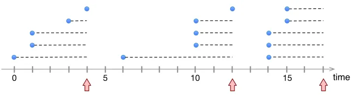
An example in Figure 1 illustrates an instance ofTCP-APand a schedule of packet transmissions.
0 5 10 15 time
Figure 1 An example ofTCP-APwith linear cost function.
point to transmission times and horizontal dashed lines represent waiting times of messages. Assume
that the cost of each packet’s transmission is 10 and that we charge for delay at rate 1 per time
unit. The schedule consists of three transmissions whose total cost is 30. The first transmitted
packet will contain 5 messages with total delay 4 + 3 + 3 + 1 + 0 = 11. The total delay of messages
in the second and third transmissions will be, respectively, 12 and 13. So the total cost of the
schedule in Figure 1 is 66.
The offline variant of TCP-AP, that is computing the optimum schedule of transmissions of
messages aggregated into packets, assuming that all arrival times of control messages are known
beforehand, can be naturally represented by an integer linear program. The optimum solution
can also be quite easily and efficiently found with dynamic programming, with the fastest known
algorithm for this problem achieving running time O(nlogn) (Aggarwal and Park 1993).
In practice, however, packet aggregation decisions must be done on the fly, in real time. This
gives rise to the online version of TCP-AP, in which an online algorithm receives information
about messages as they are released over time. At each time step, this algorithm needs to decide
whether to transmit the packet with pending messages or not, without any information about
future message releases. Online algorithms for a variety of other scheduling problems (and other
optimization problems) have been a topic of extensive study since 1980’s – see, for example, Sgall
(1998), Borodin and El-Yaniv (1998). With incomplete information about the input sequence,
an online algorithm cannot, in general, guarantee to compute an optimal solution. Thus research
in this area focuses on designing near-optimal algorithms. The quality of solutions computed by
an online algorithm is typically measured by itscompetitive ratio, which is defined (roughly) as the
worst-case ratio between its cost and the optimum cost (computed offline). Naturally, the smaller
the ratio the better.
The online variant of TCP-AP has been well studied: It is known that the optimal competitive
ratio is 2 in the deterministic case (Dooly et al. 2001), i.e., there is an algorithm that computes
10 2 3 5 8 4 r5 r4 r3 r2 r1 w s
0 5 10 time
[image:5.612.72.537.75.227.2]r1 r2 r3 r4 r5 r1 r2 r3 r5 r1 r2 r5 r4 r5 r2 r3
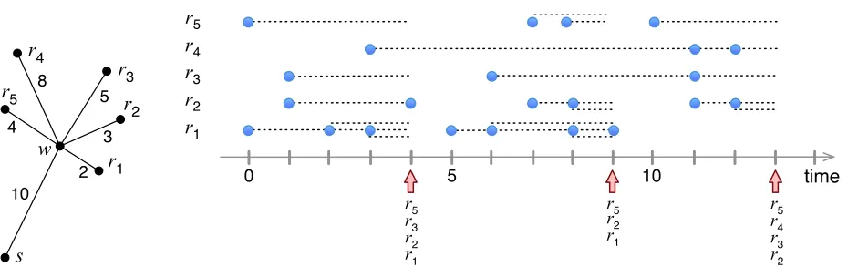
Figure 2 An example ofJRPwith linear cost function.
ratio online. With randomization, it is possible to reduce the ratio to e/(e−1)≈1.582 (Karlin
et al. 2003, Buchbinder and Naor 2009, Seiden 2000). Online variants ofTCP-APthat use different
assumptions or objective functions were also examined in the literature (Frederiksen et al. 2003,
Albers and Bals 2005).
2-level aggregation. Another optimization problem involving aggregation is the Joint
Replen-ishment Problem (JRP), well-studied in operations research. JRP models tradeoffs that arise in
supply-chain management. One such scenario involves optimizing shipments of goods from a
sup-plier to retailers, through a shared warehouse, in response to their demands. In JRP, aggregation
takes place at two levels: items addressed to different retailers can be shipped together to the
warehouse, at a fixed cost, and then multiple items destined to the same retailer can be shipped
from the warehouse to this retailer together, also at a fixed cost, which can be different for different
retailers. Pending demands accrue waiting cost until they are satisfied by a shipment. The objective
is to minimize the sum of all shipment costs and all waiting costs.
Figure 2 shows an example of an instance of JRPand a schedule. This instance has five
retail-ers r1, r2, ..., r5, the warehouse is denoted w and the supplier is denoted s. The connections are
represented by a “star” tree, shown on the left, with shipping costs associated with its edges. For
example, the shipping cost from the supplier to the warehouse is 10. On the right, requests are
represented by circles and are arranged in five rows corresponding to the retailers. There are three
shipments, at times 4, 9 and 13, marked by up-arrows, with their participating retailers listed
below. The first shipment serves retailers r1,r2,r3 and r5 and its cost is 10 + 2 + 3 + 5 + 4 = 24.
Assume that the waiting cost is equal to the time elapsed between the request and the
ship-ment that satisfies it. Then the waiting cost of the requests served by the first shipship-ment will be
Similarly toTCP-AP,JRPcan also be represented by an integer linear program (see, for example
(Buchbinder et al. 2008)). In contrast to TCP-AP, however, JRP is known to be NP-hard (Arkin
et al. 1989), and evenAPX-hard (Nonner and Souza 2009, Bienkowski et al. 2015). The currently
best approximation algorithm, due to Bienkowski et al. (2014), achieves a factor of 1.791, improving
on earlier work (Levi et al. 2005, 2008, Levi and Sviridenko 2006). In the deadline variant of JRP,
denoted JRP-D, there is no cost for waiting, but each demand needs to be satisfied before its
deadline. As shown by Bienkowski et al. (2015), JRP-D can be approximated with ratio 1.574.
For the online variant of JRP, Buchbinder et al. (2008) gave a 3-competitive algorithm using
a primal-dual scheme (improving an earlier bound of 5 by Brito et al. (2012)) and proved a lower
bound of 2.64, that was subsequently improved to 2.754 (Bienkowski et al. 2014). The optimal
competitive ratio for JRP-Dis 2 (Bienkowski et al. 2014).
Multiple-level aggregation. TCP-APandJRPcan be thought of as aggregation problems on
edge-weighted trees of depth 1 and 2, respectively. InTCP-AP, this tree is just a single edge between the
sender and the recipient. InJRP, this tree consists of the root (supplier) with one child (warehouse)
and any number of grandchildren (retailers). A shipment can be represented by a subtree of this
tree and edge weights represent shipping costs. These trees capture the general problem on trees
of depth 1 and 2, as the children of the root can be considered separately (see Section 2).
This naturally extends to trees of any depthD, where aggregation is allowed at each level.
Multi-level message aggregation has been, in fact, studied in communication networks in several contexts.
In multicasting, protocols for aggregating control messages (see, for example, Bortnikov and Cohen
(1998), Badrinath and Sudame (2000)) can be used to reduce the so-called ack-implosion, the
proliferation of control messages routed to the source. Such global approach is likely to be more
effective than applying aggregation on each link separately (which amounts to solving an instance
of theTCP-APproblem for each link). For example, the root of the tree can represent a web server
that gathers TCP acknowledgements from its open TCP connections. These TCP acknowledgement
messages are very small (40 bytes), yet each individual message needs to be processed by each node
it traverses in order to determine its route through a routing table lookup. With aggregation, only
one such processing is needed, per node, for an aggregated message that contains multiple
acknowl-edgements. As shown experimentally by Badrinath and Sudame (2000), this approach reduces
packet latency. A similar problem arises in energy-efficient data aggregation and fusion in sensor
networks (Hu et al. 2005, Yuan et al. 2003). Outside of networking, tradeoffs between the cost
of communication and delay arise in message aggregation in organizational hierarchies
(Papadim-itriou 1996). In supply-chain management, multi-level variants of lot sizing have been studied as
well (Crowston and Wagner 1973, Kimms 1997). The need to consider more tree-like (in a broad
These applications have inspired research on offline and online approximation algorithms for
multi-level aggregation problems. Becchetti et al. (2009) gave a 2-approximation algorithm for the
deadline case. (See also (Brito et al. 2012).) Pedrosa (2013) showed, adapting an algorithm of Levi
et al. (2006) for the multi-stage assembly problem, that there is a (2 +ε)-approximation algorithm
for general waiting cost functions, where εcan be made arbitrarily small.
In the online case, Khanna et al. (2002) gave a rent-or-buy solution (that serves a group of
requests once their waiting cost reaches the cost of their service) and showed that their algorithm
isO(logW)-competitive, whereW is the sum of all edge weights. However, they assumed that each
request has to wait at least one time unit. This assumption is crucial for their proof, as demonstrated
by Brito et al. (2012), who showed that the competitive ratio of a rent-or-buy strategy is Ω(D),
even for paths with D edges. The same assumption of a minimal cost for a request and a ratio
dependent on the edge-weights is also essential in the work of Vaya (2012), who studies a variant
of the problem with bounded bandwidth (the number of packets that can be served by a single
edge in a single service).
The existence of a primal-dual (2 +ε)-approximation algorithm (Pedrosa 2013, Levi et al. 2006)
for the offline problem suggests the possibility of constructing an online algorithm along the lines
of the scheme by Buchbinder and Naor (2009). Nevertheless, despite substantial effort of many
researchers, the online multi-level setting remains wide open. This is perhaps partly due to
impos-sibility of direct emulation of the cleanup phase in primal-dual offline algorithms in the online
setting, as this cleanup is performed in the “reverse time” order.
The case when the tree is just a path has also been studied. An offline polynomial-time algorithm
that computes an optimal schedule was given by Bienkowski et al. (2013). For the online variant,
Brito et al. (2012) gave an 8-competitive algorithm. This result was improved by Bienkowski et al.
(2013) who showed that the competitive ratio of this problem is between 2 +φ≈3.618 and 5.
A related problem of integrated scheduling and distribution has also been studied in the online
setting (Azar et al. 2016): It resembles JRP, but in our terms, actually corresponds to a 1-level
tree with multiple leaves. While services of those are independent, there is an interplay at the root
of the tree, as each request has to be processed for its own specified amount of time at the root
before being serviced — like in lot-sizing or JRP, these can be thought of as re-stocking orders, but
fulfilled directly by a manufacturer once the items are produced. Azar et al. (2016) consider linear
waiting costs (and preemptive scheduling/production), but, in principle, one could study arbitrary
waiting functions and allow complex aggregation in shipment, as we do in this work.
1.1. Our Contributions
We study online competitive algorithms for multi-level aggregation. Minor technical differences
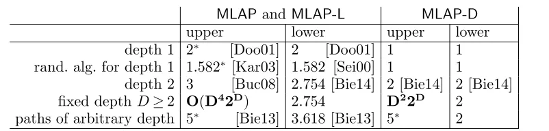
MLAP andMLAP-L MLAP-D
upper lower upper lower
depth 1 2∗ [Doo01] 2 [Doo01] 1 1
rand. alg. for depth 1 1.582∗ [Kar03] 1.582 [Sei00] 1 1
depth 2 3 [Buc08] 2.754 [Bie14] 2 [Bie14] 2 [Bie14]
fixed depthD≥2 O(D42D) 2.754 D22D 2
[image:8.612.113.514.73.169.2]paths of arbitrary depth 5∗ [Bie13] 3.618 [Bie13] 5∗ 2
Table 1 Previous and current bounds on the competitive ratios forMLAPfor trees of various depths. Ratios written in bold are shown in this paper. Except the second line in the table, all bounds are for deterministic
algorithms. The references to particular papers were shortened in the following way: [Sei00] (Seiden 2000), [Doo01] (Dooly et al. 2001), [Kar03] (Karlin et al. 2003), [Buc08] (Buchbinder et al. 2008), [Bie13] (Bienkowski et al. 2013), and [Bie14] (Bienkowski et al. 2014). Unreferenced results are either immediate consequences of other entries in the table or trivial observations. Asterisked ratios represent results forMLAPwith arbitrary waiting cost
functions, which, though not explicitly stated in the respective papers, are straightforward extensions of the corresponding results forMLAP-L. Some values in the table are approximations: 1.582 represents e/(e−1) and 3.618
represents 2 +φ, whereφis the golden ratio.
(2002), also extending the deadline variant (Becchetti et al. 2009) and the assembly problem
(Levi et al. 2006). We have decided to choose a more generic terminology to emphasize general
applicability of our model and techniques.
Formally, in our model, an instance of the problem consists of a tree T with positive weights
assigned to edges, and a set Rof requests that arrive in the nodes of T over time. These requests
are served by subtrees rooted at the root ofT. Such a subtreeX serves all requests pending at the
nodes ofX at cost equal to the total weight of X. Each request incurs a waiting cost, defined by
a non-negative and non-decreasing function of time, which may be different for each request. The
objective is to minimize the sum of the total service and waiting costs. We call this theMulti-Level
Aggregation Problem (MLAP).
In most earlier papers on aggregation problems, the waiting cost function is linear, that is, it is
assumed to be simply the delay between the times when a request arrives and when it is served. We
denote this version by MLAP-L. However, most of the algorithms for this model extend naturally
to arbitrary cost functions. Another variant is MLAP-D, where each request is given a certain
deadline, has to be served before or at its deadline, and there is no penalty associated with waiting.
This can be modeled by the waiting cost function that is 0 up to the deadline and +∞afterwards.
In this paper, we mostly focus on the online version of MLAP, where an algorithm needs to
produce a schedule in response to requests that arrive over time. When a request appears, its
waiting cost function is also revealed. At each timet, the online algorithm needs to decide whether
to generate a service tree at this time, and if so, which nodes should be included in this tree.
The main result of our paper is anO(D42D)-competitive algorithm forMLAPfor trees of depthD,
No competitive algorithms have been known so far for onlineMLAPfor arbitrary depth trees, even
for the special case of MLAP-Don trees of depth 3.
For both results we use a reduction, described in Section 3, of the general problem to the special
case of trees with rapidly decreasing weights. For such trees we then provide an explicit competitive
algorithm. While our algorithm is compact and elegant, it is not a straightforward extension of the
2-level algorithm. (In fact, we have been able to show that na¨ıve extensions of the latter algorithm
are not competitive.) It is based on carefully constructing a sufficiently large service tree whenever
it appears that an urgent request must be served. The specific structure of the service tree is then
heavily exploited in an amortization argument that constructs a mapping from the algorithm’s
cost to the cost of the optimal schedule. We believe that these three new techniques: the reduction
to trees with rapidly decreasing weights, the construction of the service trees, and our charging
scheme, will be useful in further studies of online aggregation problems.
Finally, in Section 6, we discuss several technical issues concerning the use of general functions
as waiting costs inMLAP. In particular, when presenting our algorithms forMLAPwe assume that
all waiting cost functions are continuous (which cannot directly capture some interesting variants
of MLAP). This is done, however, only for technical convenience; as explained in Section 6, these
algorithms can be extended to left-continuous functions, which allows us to model MLAP-D as a
special case ofMLAP. We also consider two alternative models forMLAP: the discrete-time model
and the model where not all requests need to be served, showing that our algorithms can be
extended to these models as well.
Notes. An extended abstract of this work appeared in the proceedings of 24th Annual
Euro-pean Symposium on Algorithms (ESA) (Bienkowski et al. 2016). (Other results announced in
(Bienkowski et al. 2016) will be published in a separate companion paper.) In a subsequent work,
Azar et al. (2017) study a more general service problem with delays. This problem includesMLAP
as a special case when in addition to the requests from MLAP, we repeat many requests to the
root of the tree. The results of Azar et al. (2017) then imply O(DO(1)) competitive algorithm for
MLAP. Finally, Buchbinder et al. (2017) improve the competitive ratio for MLAP-D (the variant
with deadlines) to O(D). Their approach uses a more subtle charging argument, combined with
a reduction to the case with rapidly decreasing weights (similar to ours), showing that some of
the ideas introduced in this paper could indeed be helpful for ultimately determining the tight
competitive ratio for MLAP.
2. Preliminaries
Weighted trees. Let T be a tree with root r. The parent of a node x is denoted parent(x). The
depth of x, denoteddepth(x), is the number of edges on the simple path fromr tox. In particular,
For any set of nodes Z⊆ T and a node x, Zx denotes the set of all descendants of x in Z; in
particular, Tx is the induced subtree of T rooted at x. Furthermore, Zi denotes the set of nodes
in Z of depth i in tree T. Let also Z<i=Si−1
j=0Z
j and Z≤i=Z<i∪Zi. These notations can be
combined with the notationZx, so, e.g.,Zx<iis the set of all descendants ofxthat belong toZ and
whose depth inT is smaller thani.
We will deal with weighted trees in this paper. For x6=r, by `x or`(x) we denote the weight of
the edge connecting nodex to its parent. (In a typical application this weight would represent the
length or the cost of traversing this edge.) For the sake of convenience, we will often refer to `x as
the weight of x. We assume that all these weights are positive. We extend this notation to r by
setting `r= 0. IfZ is any set of nodes of T, then the weight of Z is`(Z) =
P
x∈Z`x.
Definition ofMLAP. Arequest ρis specified by a tripleρ= (σρ, aρ, ωρ), whereσρis the node ofT
in which ρ is issued, aρ is the non-negative arrival time of ρ, and ωρ is the waiting cost function
of ρ. We assume that ωρ(t) = 0 for t≤aρ and ωρ(t) is non-decreasing for t≥aρ. MLAP-L is the
variant of MLAP with linear waiting costs; that is, for each request ρ we have ωρ(t) =t−aρ, for
t≥aρ. In MLAP-D, the variant with deadlines, we haveωρ(t) = 0 for aρ≤t≤dρ and ωρ(t) = +∞
for t > dρ, where dρ is called the deadline of request ρ. We assume that all the deadlines in the
given instance are distinct. This may be done without loss of generality, as in case of ties we can
modify the deadlines by infinitesimally small perturbations.
In our algorithm forMLAPwith general costs, we will be assuming that all waiting cost functions
are continuous. This is only for technical convenience and we discuss more general waiting cost
functions in Section 6; we also show there thatMLAP-Dcan be considered a special case ofMLAP,
and that our algorithms can be extended to the discrete-time model.
Aserviceis a pair (X, t), whereXis a subtree ofT rooted atrandtis the time of this service. We
will occasionally refer toX as the service tree (or just service) at timet, or even omittaltogether
if it is understood from context.
An instance J =hT,Riof the Multi-Level Aggregation Problem (MLAP) consists of a weighted
tree T with root r and a set R of requests arriving at the nodes of T. A schedule is a set S of
services. For a requestρ, let (X, t) be the service inSwith minimaltsuch thatσρ∈X and t≥aρ.
We then say that (X, t) serves ρ and the waiting cost of ρ in S is defined aswcost(ρ,S) =ωρ(t).
Furthermore, the requestρ is calledpending at all times in the interval [aρ, t]. ScheduleS is called
feasible if all requests in Rare served by S.
The cost of a feasible schedule S, denotedcost(S), is defined by
where scost(S) is the total service cost and wcost(S) is the total waiting cost, that is
scost(S) = X
(X,t)∈S
`(X) and wcost(S) =X
ρ∈R
wcost(ρ,S).
The objective ofMLAP is to compute a feasible scheduleS forJ with minimum cost(S).
Online algorithms. We use the standard and natural definition of online algorithms and the
competitive ratio. We assume the continuous time model. The computation starts at time 0 and
from then on the time gradually progresses. At any time t new requests can arrive. If the current
time is t, the algorithm has complete information about the requests that arrived up until timet,
but has no information about any requests whose arrival times are after time t. The instance
includes a time horizon H that is not known to the online algorithm, which is revealed only at
time t=H. At time H, all requests that are still pending must be served. (In the offline case, H
can be assumed to be equal to the maximum request arrival time.)
IfAis an online algorithm andc≥1, we say thatAisc-competitive ifcost(S)≤c·opt(J) for any
instanceJ ofMLAP, whereSis the schedule computed byAonJ andopt(J) is the optimum cost
forJ. (Note that the definition of competitiveness in the literature often allows an additive error
term, independent of the request sequence. For our algorithms, this additive term is not needed.)
Quasi-root assumption. Throughout the paper we will assume that r, the root of T, has only
one child. This is without loss of generality, because if we have an algorithm (online or offline) for
MLAP on such trees, we can apply it independently to each child of r and its subtree. This will
give us an algorithm forMLAPon arbitrary trees with the same performance. From now on, let us
call the single child of r the quasi-root of T and denote it by q. Note that q is included in every
(non-trivial) service. Requests atr can be serviced immediately at cost 0, so we can simply assume
that there are no such requests in R.
Urgency functions. When choosing nodes for inclusion in a service, our online algorithms give
priority to those that are most “urgent”. ForMLAP-D, naturally, urgency of nodes can be measured
by their deadlines, where a deadline of a node v is the earliest deadline of a request pending in
the subtree Tv, i.e., the induced subtree rooted at v. But for the arbitrary instances of MLAPwe
need a more general definition of urgency, which takes into account the rate of increase of the
waiting cost in the future. To this end, each of our algorithms will use some urgency function
f:T →R∪ {+∞}, which also depends on the set of pending requests and the current time step,
and which assigns some time value to each node. The earlier this value, the more urgent the node is.
Formally, for MLAP-D, we define the function dt(v) for any time t as follows. For any node v,
dt(v) is the earliest deadline among all requests inT
v that are pending for the algorithm at timet;
if there is no pending request inTv, we setdt(v) = +∞. We usedt as the urgency function at time
Definition 1. Letf be an urgency function,Abe a set of nodes inT andβ≥0 be a real number.
Then,Urgent(A, β, f) is the smallest set of nodes inA such that
1. for allu∈Urgent(A, β, f), and v∈A−Urgent(A, β, f) we have f(u)≤f(v), and
2. either `(Urgent(A, β, f))≥β orUrgent(A, β, f) =A.
Intuitively, Urgent(A, β, f) is the set of nodes obtained by choosing the nodes from A in order
of their increasing urgency value, until either their total weight exceeds β or we run out of nodes
from A. In case of ties in the values of f, there may be multiple choices for Urgent(A, β, f); we
choose among them arbitrarily.
3. Reduction to
α
-Decreasing Trees
One basic intuition that emerges from earlier works on trees of depth 2 (Buchbinder et al. 2008,
Brito et al. 2012, Bienkowski et al. 2014) is that the hardest case of the problem is when `q,
the weight of the quasi-root, is much larger than the weights of leaves. For arbitrary depth trees,
the hard case is when the weights of nodes quickly decrease with their depth. We show that this
is indeed the case, by defining the notion of α-decreasing trees that captures this intuition and
showing thatMLAPreduces to the special case ofMLAPfor suchα-decreasing trees, increasing the
competitive ratio by a factor of at most Dα. The value of α used in our algorithms will be fixed
later. This is a general result, not limited only to algorithms in our paper.
Definition 2. Fixα≥1. A treeT is α-decreasing if for any nodeu different from the root of T
and for any child v of u, it holds that`u≥α·`v.
Note that the α-decreasing property is one of the conditions of α-HST (a hierarchically
well-separated tree with separation α, see, e.g., (Bartal 1996)). That is, any α-HST is also an α
-decreasing tree. However, for our purposes we do not require that the edge weight from any node
to its children is the same, which is required byα-HST.
Theorem 1. If there exists ac-competitive algorithmAforMLAP(resp.MLAP-D) onα-decreasing
trees (where c can be a function of D, the tree depth), then there exists a Dαc-competitive
algo-rithm B for MLAP(resp. MLAP-D) on arbitrary trees.
Proof. Fix the underlying instanceJ = (T,R), whereT is a tree andRis a sequence of requests
inT. In our reduction, we convertT to anα-decreasing treeT0 on the same set of nodes. We then
show that any service onT is also a service onT0 of the same cost and, conversely, that any service
on T0 can be converted to a slightly more expensive service onT.
We start by constructing an α-decreasing tree T0 on the same set of nodes. For any node u∈
`w≥α·`u; if no suchwexists, we takew=r. The length of an edge fromuto its parent remains`u.
Note that T0 may violate the quasi-root assumption, which does not change the validity of the
reduction, as we may use independent instances of the algorithm for each child of r in T0. Since
in T0 each node u is connected to one of its ancestors from T, it follows that T0 is a tree rooted
atr with depth at most D. Obviously,T0 is α-decreasing.
The construction implies that if a set of nodesXis a service subtree ofT, then it is also a service
subtree for T0 of the same cost. (However, note that the actual topology of the trees with node
setX inT andT0 may be very different. For example, ifα= 5 andT is a path with costs (starting
from the leaf) 1,2,22, ...,2D, then in T0 the node of weight 2i is connected to the node of weight
2i+3, except for the last three nodes that are connected tor. Thus the resulting tree consists of three
paths ending atr with roughly the same number of nodes. In particular,X inT0 may now contain
paths without any request.) Therefore, any schedule forJ is also a schedule forJ0= (T0,R), which
gives us thatopt(J0)≤opt(J).
The algorithmBforT is defined as follows: On a request sequenceR, we simulateAforRinT0,
and wheneverAcontains a serviceX,Bissues the serviceX0⊇X, created fromX as follows: Start
with X0=X. Then, for each u∈X− {r}, if w is the parent ofu inT0, then add to X0 all inner
nodes on the path fromu tow inT. By the construction of T0, for each u we add at mostD−1
nodes, each of weight less thanα·`u. It follows that `(X0)≤((D−1)α+ 1)`(X)≤Dα·`(X).
In total, the service cost ofBis at mostDαtimes the service cost ofA. Any request served byA
is served by B at the same time or earlier, thus the waiting cost of B is at most the waiting cost
of A(resp. for MLAP-D,B produces a valid schedule forJ). Since Ais c-competitive, we obtain
cost(B,J)≤Dα·cost(A,J0)≤Dαc·opt(J0)≤Dαc·opt(J),
and thusB isDαc-competitive.
4. A Competitive Algorithm for
MLAP-D
In this section we present our online algorithm forMLAP-Dwith competitive ratio at most D22D.
To this end, we will give an online Algorithm OnlTreeD that achieves competitive ratio cα=
(2 + 1/α)D−1forα-decreasing trees. Together with the reduction given in the previous section, this will imply the following result.
Theorem 2. There exists aD22D-competitive online algorithm for MLAP-D on trees of depth D.
Proof. Applying Theorem 1 to Algorithm OnlTreeD, we obtain that there exists aDαcα= Dα(2 + 1/α)D−1-competitive algorithm for general trees. For D≥2, choosing α=D/2 yields a competitive ratio bounded by 1
2D
22D−1·(1 + 1/D)D≤ 1 4D
22D·e≤D22D. For D= 1 there is
4.1. Intuition
Consider the optimal 2-competitive algorithm for MLAP-D for trees of depth 2 (Bienkowski et al.
2014). Assume that the tree is α-decreasing, for some large α. (Thus `q `v, for each leaf v.)
Whenever a pending request reaches its deadline, this algorithm serves a subtree X consisting
ofr, qand the set of leaves with the earliest deadlines and total weight of about`q. This is a natural
strategy: We have to pay at least `q to serve the expiring request, so including an additional
set of leaves of total weight `q can at most double our overall cost. At the same time, assuming
that no new requests arrive, serving this X can significantly reduce the cost in the future, since
servicing these leaves individually is expensive: it would cost `v+`q per each leafv, compared to
the incremental cost of`v to include v inX.
For α-decreasing trees with three levels (that is, for D= 3), we may try to iterate this idea.
When constructing a service treeX, we start by adding to X the set of most urgent children of q
whose total weight is roughly`q. Now, when choosing nodes of depth 3, we have two possibilities:
(1) for eachv∈X− {r, q} we can add toX its most urgent children of combined weight `v (note
that their total weight will add up to roughly `q, because of the α-decreasing property), or (2)
from the set ofall children of the nodes in X− {r, q}, add toX the set of total weight roughly `q
consisting of (globally) most urgent children.
It is not hard to show that option (1) does not lead to a constant-competitive algorithm: The
counter-example involves an instance with one node w of depth 2 having many children with
requests with early deadlines and all other leaves having requests with very distant deadlines.
Assume that`q=α2,`w=α, and that each leaf has weight 1. The example forces the algorithm to
serve the children ofw in small batches of size αwith cost more thanα2 per batch orα per each
child ofw, while the optimum can serve all the requests in the children ofwat once with costO(1)
per request, giving a lower bound Ω(α) on the competitive ratio. (The requests at other nodes can
be ignored in the optimal solution, as we can keep repeating the above strategy in a manner similar
to the lower-bound technique presented, e.g., by Buchbinder et al. (2008) or by Bienkowski et al.
(2013).) A more intricate example shows that option (2) by itself is not sufficient to guarantee
constant competitiveness either.
The idea behind our algorithm, for trees of depth D= 3, is to doboth (1) and (2) to obtain X.
This increases the cost of each service by a constant factor, but it protects the algorithm against
both bad instances. The extension of our algorithm to depthsD >3 carefully iterates the process
of constructing the service tree X, to ensure that for each nodev∈X and for each levelibelowv
4.2. Algorithm OnlTreeD
At any timetwhen some request expires, that is whent=dt(q) for the quasi-rootq, the algorithm
serves a subtree X constructed by first initializingX={r, q}, and then incrementally augmenting
X according to the following pseudo-code:
for eachdepth i= 2, . . . , D
Zi← set of all children of nodes in Xi−1
for eachv∈X<i
U(v, i, t)←Urgent(Zi v, `v, dt)
X←X∪U(v, i, t)
In other words, at depth i, we restrict our attention toZi, the children of all the nodes inXi−1, i.e., of the nodes that we have previously selected to X at level i−1. (We start with i= 2 and
X1={q}.) Then we iterate over all v∈X<i and we add to X the set U(v, i, t). U(v, i, t) itself is
created by taking nodes fromTi
v (descendants ofvat depthi) whose parents are inX, one by one,
in the order of increasing deadlines, stopping when either their total weight exceeds`v or when we
run out of such nodes. SinceT isα-decreasing, each added node has weight at most`v/α, and thus
the total weight ofU(v, i, t) is at most`v+`v/α. Note that added sets do not need to be disjoint.
The constructed set X is a service tree, as we are adding to it only nodes that are children of
the nodes already in X.
Let ρ be the request triggering the service at timet, i.e., satisfying dρ=t. (By the assumption
about different deadlines, ρ is unique.) Naturally, all the nodes u on the path from r to σρ have
dt(u) =tand qualify as the most urgent, thus the nodeσ
ρis included inX. Therefore every request
is served before its deadline.
4.3. Analysis
Intuitively, it should be clear that Algorithm OnlTreeD cannot have a better cost-to-optimum
ratio than`(X)/`q: If all requests are inq, the optimum will serve onlyq, while our algorithm uses
a set X with many nodes that turn out to be useless. As we will show, via an iterative charging
argument, the ratio `(X)/`q is actually achieved by the algorithm.
Recall that cα= (2 + 1/α)D−1. We now prove a bound on the cost of the service tree.
Lemma 1. Let X be the service tree produced by Algorithm OnlTreeD at time t. Then `(X)≤
cα·`q.
Proof. We prove by induction that `(X≤i)≤(2 + 1/α)i−1`
The base case of i= 1 is trivial, as X≤1={r, q} and `
r= 0. For i≥2, Xi is the union of the
sets U(v, i, t) over all nodes v∈X<i. Recall that by our construction, `(U(v, i, t))≤`
v+`v/α=
(1 + 1/α)`v. Therefore, by the inductive assumption, we get that
`(X≤i)≤(1 + (1 + 1/α))·`(X<i)
≤(2 + 1/α)·(2 + 1/α)i−2`q= (2 + 1/α)i−1`q,
proving the induction step and completing the proof that`(X)≤cα·`q.
The competitive analysis uses a charging scheme. Fix some optimal schedule S∗. Consider a ser-vice (X, t) of AlgorithmOnlTreeD. We will identify inX a subset of “critically overdue” nodes
(to be defined shortly) of total weight at least `q≥`(X)/cα, and we will show that for each such
critically overdue nodev we can charge the portion`v of the service cost ofX to an earlier service
in S∗ that contains v. Further, each occurrence of v in the services of S∗ will be charged at most once in this way. This implies that the total cost of our algorithm is at mostcα times the optimal
cost, giving us an upper bound of cα on the competitive ratio forα-decreasing trees.
In the proof, by nost
v we denote the time of the first service in S ∗
that includes v and is strictly
after time t; we also let nost
v= +∞ if no such service exists (nosstands for next optimal service).
For a service (X, t) of the algorithm, we say that a nodev∈X isoverdue at timetifdt(v)<nost v.
Servicing of such v is delayed in comparison to S∗, because S∗ must have served v before or at timet. Note also thatr andq are overdue at timet, asdt(r) =dt(q) =tby the choice of the service
time. We definev∈X to be critically overdue at timetif (i) v is overdue att, and (ii) there is no
other service of the algorithm in the time interval (t,nost
v) in whichv is overdue.
We are now ready to define the charging for a service (X, t). For each v∈X that is critically
overdue, we charge its weight `v to the last service ofv inS ∗
before or at time t. This charging is
well-defined as, for each overduev, there must exist a previous service ofv inS∗. The charging is obviously one-to-one because between any two services in S∗ that involvev there may be at most one service of the algorithm in which v is critically overdue. The following lemma shows that the
total charge from X is large enough.
Lemma 2. Let (X, t) be a service of Algorithm OnlTreeD and suppose that v∈X is overdue at
timet. Then the total weight of critically overdue nodes in Xv at time t is at least `v.
Proof. The proof is by induction on the depth of Tv, the induced subtree rooted at v.
The base case is when Tv has depth 0, that is when v is a leaf. We show that in this case
v must be critically overdue, which implies the conclusion of the lemma. Towards contradiction,
suppose that there is some other service at time t0∈(t,nost
r
q
w
σ
ρ [image:17.612.147.464.78.231.2]X
Y
v
x
i
U(v,i,t)
Figure 3 Illustration of the proof of Lemma 2.
leaf, after the service at time tthere are no pending requests in Tv={v}. Asv is overdue at time
t0, we have dt0(v)<nost0 v =nos
t
v and this implies that there is a request ρ with σρ=v such that t < aρ≤dρ<nostv. But this is not possible, becauseS
∗
does not servevin the time interval (t,nost v).
Thus v is critically overdue and the base case holds.
Assume now that v is not a leaf, and that the lemma holds for all descendants of v. If v is
critically overdue, the conclusion of the lemma holds.
Thus we can now assume that v is not critically overdue. This means that there is a service
(Y, t0) of Algorithm OnlTreeD with t < t0<nostv which contains v and such that v is overdue
att0. Thus nost v=nos
t0 v.
Let ρ be the request withdρ=dt 0
(v), i.e., the most urgent request inTv at time t0.
We claim that aρ≤t, i.e.,ρarrived no later than at time t. Indeed, sincevis overdue at timet0,
it follows that dρ<nost 0 v =nos
t
v. The optimal scheduleS ∗
cannot serveρ after timet, asS∗ has no service from v in the interval (t, dρ]. Thus S
∗
must have served ρ before or att, and henceaρ≤t,
as claimed.
Now consider the path from σρ tov in Y. (See Figure 3.) As ρ is pending for the algorithm at
timet and ρ is not served by (X, t), it follows that σρ6∈X. Letw be the last node on this path in
Y −X. Then wis well-defined andw6=v, asv∈X. Letibe the depth of w. Note that the parent
of wis in X<i
v , so w∈Z
i in the algorithm whenX is constructed.
The node σρ is in Tw and ρ is pending at t, thus we have dt(w)≤dρ. Since w∈Zi but w was
not added to Xat timet, we have that`(U(v, i, t))≥`v and eachx∈U(v, i, t) is at least as urgent
asw. This implies that suchx satisfies
dt(x)≤dt(w)≤d
ρ<nost 0 v =nos
t v≤nos
t x,
and thusxis overdue at timet. By the inductive assumption, the total weight of critically overdue
obtain that the total weight of critically overdue nodes inXvis at least`(U(v, i, t))≥`v, completing
the proof.
Now consider a service (X, t) of the algorithm. The quasi-rootqis overdue at timet, so Lemmata 2
and 1 imply that the charge from (X, t) is at least `q ≥`(X)/cα. Since each node in any service
in S∗ is charged at most once, we conclude that Algorithm OnlTreeD iscα-competitive for any α-decreasing treeT.
5. A Competitive Algorithm for
MLAP
In this section, we show that there is an online algorithm for MLAP whose competitive ratio for
trees of depth D is O(D42D). As in Section 4, we will assume that the tree T in the instance is
α-decreasing and present a competitive algorithm for such trees, which will imply the existence of
a competitive algorithm for arbitrary trees by using Theorem 1 and choosing an appropriate value
of α.
5.1. Preliminaries and Notations
Recall that ωρ(t) denotes the waiting cost function of a request ρ. As explained in Section 2, we
assume that the waiting cost functions are continuous. (In Section 6, we discuss how to extend
our results to arbitrary waiting cost functions.) We will overload this notation, so that we can talk
about the waiting cost of a set of requests or a set of nodes. Specifically, for a set P of requests
and a setZ of nodes, let
ωP(Z, t) =
X
ρ∈P:σρ∈Z ωρ(t).
Thus ωP(Z, t) is the total waiting cost of the requests from P that are issued inZ. We sometimes
omitP, in which case the notation refers to the set of all requests in the instance, that isω(Z, t) =
ωR(Z, t). Similarly, we omitZ when Z contains all nodes, that isωP(t) =ωP(T, t).
Maturity time. In our algorithm forMLAP-D in Section 4, the times of services and the urgency
of nodes are both naturally determined by the deadlines. ForMLAPwith continuous waiting costs
there are no hard deadlines. Nevertheless, we can still introduce the notion of maturity time of
a node, which is, roughly speaking, the time when some subtree rooted at this node has its waiting
cost equal to its service cost; this subtree is then called mature. This maturity time will be our
urgency function, as discussed earlier in Section 2. We use the maturity time in two ways: first, the
maturity times of the quasi-root determine the service times, and second, maturity times of other
nodes are used to prioritize them for inclusion in the service trees. We now proceed to define these
Consider some timetand any setP⊆ Rof requests and a subtreeZ ofT (not necessarily rooted
atr).Z is calledP-mature at timet ifωP(Z, t)≥`(Z). Let
µP(Z) = arg min
t {ωP(Z, t)≥`(Z)}.
That is,µP(Z) is the earliest timeτ at whichZisP-mature; if suchτ does not exist, we setµP(Z) =
+∞. Since ωP(Z,0) = 0, `(Z)≥0, and ωP(Z, t) is a non-decreasing and continuous function oft,
µP(Z) is well-defined.
In the following definition, a conditionZv Tv denotes that a set of nodesZ is not only a subtree
of Tv, but is also itself rooted atv. Consider any nodev and any set P⊆ Rof requests. Let
MP(v) = min ZvTv
µP(Z) and (1)
CP(v) = arg min ZvTv
µP(Z). (2)
MP(v) is called the P-maturity time of v and CP(v) is called the P-critical subtree rooted at v;
if there are more such trees, we choose one arbitrarily. From the above definitions, we have that
ωP(CP(v), MP(v)) =`(CP(v)).
The following simple lemma guarantees that the maturity time of any node in the P-critical
subtree CP(v) is upper bounded by the maturity time of v.
Lemma 3. Let u∈CP(v) and let Y = (CP(v))u be the induced subtree of CP(v) rooted at u. Then MP(u)≤µP(Y)≤MP(v).
Proof. The first inequality follows directly from the definition of MP(u). To show the second
inequality, we proceed by contradiction. Lett=MP(v). If the second inequality does not hold, then
u6=v and ωP(Y, t)< `(Y). Take Y0=CP(v)−Y, which is a tree rooted atv. SinceωP(CP(v), t) = `(CP(v)), we have thatωP(Y0, t) =ωP(CP(v), t)−ωP(Y, t)> `(CP(v))−`(Y) =`(Y0). This in turn
implies thatµP(Y0)< t, which is a contradiction with the definition oft=MP(v).
We stress that the concepts of maturity times and critical subtrees are defined above abstractly
with respect to arbitrary sets P of requests, and are independent of the online algorithm. Yet,
naturally, in our algorithm and its analysis, in most cases thisP will represent the set of requests
pending for the algorithm at a given time. Thus, for any time t, we will also introduce simplified
notationsMt(v) andCt(v) to denote the timeM
P(v) and theP-critical subtreeCP(v), whereP is
the set of requests pending for the algorithm at timet; if it so happens that the algorithm schedules
a service at some time t, then this P represents the set of requests that are pending at time t
right before this service is executed. Note that in general it is possible that Mt(v)< t. However,
our algorithm will maintain the invariant that for the quasi-rootq we will haveMt(q)≥tat each
5.2. Algorithm
We now describe our algorithm forα-decreasing trees. A service will occur at each maturity time of
the quasi-rootq (with respect to the pending requests), that is at each timetfor which t=Mt(q).
At such a time, the algorithm chooses a service that contains the critical subtree C=Ct(q) of q
and an extra set E, whose service cost is not much more expensive than that ofC. The extra set
is constructed similarly as in AlgorithmOnlTreeD, where the urgency of nodes is now measured
by their maturity time. In other words, our urgency function is now f=Mt (see Section 2.) As
before, this extra set will be a union of a system of setsU(v, i, t) fori= 2, . . . , D,andv∈C<i∪E<i,
except that now, for technical reasons, the setsU(v, i, t) will be mutually disjoint and also disjoint
from C.
Algorithm OnlTree. At any time t such that t=Mt(q), serve the set X=C∪E constructed
according to the following pseudo-code:
C←Ct(q)∪ {r}
E← ∅
for eachdepth i= 2, . . . , D
Zi← set of all nodes inTi−C whose parent is in C∪E
for eachv∈(C∪E)<i
U(v, i, t)←Urgent(Zi
v, `v, Mt) E←E∪U(v, i, t)
Zi←Zi−U(v, i, t)
At the end of the instance (when t=H, the time horizon), if there are any pending requests,
OnlTreeissues the last service that contains all nodesv with a pending request inTv.
Note that X=C∪E is indeed a service tree, as it contains r, q and we are adding to it only
nodes that are children of the nodes already in X. The initial choice and further changes of Zi
imply that the sets U(v, i, t) are pairwise disjoint and disjoint from C — a fact that will be useful
in our analysis.
We also need the following fact.
Lemma 4. Suppose that Algorithm OnlTree issues a service at a time t, that is Mt(q) =t. Let
P0 denote the set of requests pending at time t and not served at timet. Then M
P0(q)> t.
Proof. Consider any subtree Y of T rooted atq. It is sufficient to show that ωP0(Y, t)< `(Y).
We claim that the following relations hold:
ω(Ct(q)∪Y, t)≥ω(Ct(q), t) +ωP0(Y, t) (3)
ω(Ct(q)∪Y, t)≤`(Ct(q)∪Y) (5)
`(Ct(q)∪Y)< `(Ct(q)) +`(Y) (6)
Indeed, inequality (3) is true because each request pending at time t in Ct(q)∪Y contributes to
at most one of the terms on the right-hand side: if it is in Ct(q) then it’s served at time t, so it
cannot be in P0. Inequalities (4) and (5) follow from the assumption that Mt(q) =tand from the
definition ofCt(q). (Observe thatCt(q)∪Y v T
q, that isCt(q)∪Y is also a candidate for a critical
set in (2).) Inequality (6) holds becauseCt(q) and Y both contain q with `(q)>0.
Combining (3)-(6), we obtain
`(Ct(q)) +ωP0(Y, t) =ω(Ct(q), t) +ωP0(Y, t)
≤ω(Ct(q)∪Y, t)
≤`(Ct(q)∪Y)< `(Ct(q)) +`(Y),
and ωP0(Y, t)< `(Y) follows.
Corollary 1. At any time t we have Mt(q)≥t.
Proof. The statement holds trivially at the beginning, at timet= 0. In any time interval without
new requests released nor services, the inequality Mt(q)≥t is preserved by the definition of the
service times and continuity of waiting cost functions. Releasing a requestρat a timeaρ=tcannot
decrease Mt(q) to belowt, because the waiting cost function ofρ is identically 0 up tot, and thus
releasing ρ does not change the waiting costs at time t or before. Finally, Lemma 4 implies that
the inequality is also preserved when a service occurs.
Corollary 1 shows that the sequence of service times is non-decreasing and thus the definition of
the algorithm is sound. In fact Lemma 4 even shows that no two services can occur at the same
time.
5.3. Competitive Analysis
We now present the proof that there is a O(D42D)-competitive algorithm for MLAP for trees of
depth D. The overall argument is quite intricate, so we will start by summarizing its main steps:
• First, as explained earlier, we will assume that the tree T in the instance is α-decreasing.
For such T we will show that Algorithm OnlTree has competitive ratio O(D2cα), where cα=
• For α-decreasing trees, the bound of the competitive ratio of Algorithm OnlTree involves
four ingredients:
— We show (in Lemma 5) that the total cost of Algorithm OnlTree is at most twice its
service cost.
— Next, we show that the service cost of AlgorithmOnlTreecan be bounded (within a
con-stant factor) by the total cost of all critical subtrees Ct(q) of the service trees in its schedule.
— To facilitate the estimate of the adversary cost, we introduce the concept of a
pseudo-schedule denoted S. The pseudo-schedule S is a collection of pseudo-services, which include the
services from the original adversary scheduleS∗. We show (in Lemma 7) that the adversary pseudo-schedule has service cost not larger thanDtimes the cost ofS∗. Using the pseudo-schedule allows us to ignore the waiting cost in the adversary’s schedule.
— With the above bounds established, it remains to show that the total cost of critical
sub-trees in the schedule of Algorithm OnlTree is within a constant factor of the service cost of
the adversary’s pseudo-schedule. This is accomplished through a charging scheme that charges
nodes (or, more precisely, their weights) from each critical subtree of AlgorithmOnlTreeto their
appearances in some earlier adversary pseudo-services.
Two auxiliary bounds. We now assume that T is α-decreasing and proceed with our proof,
according to the outline above.
The definition of the maturity time implies that the waiting cost of all the requests served is
at most the service cost `(X), as otherwiseX would be a good candidate for a critical subtree at
some earlier time. Denoting byS the schedule computed by AlgorithmOnlTree, we thus obtain: Lemma 5. cost(S)≤2·scost(S).
Using Lemma 5, we can restrict ourselves to bounding the service cost, losing at most a factor
of 2. We now bound the cost of a given serviceX; recall that cα= (2 + 1/α)D−1.
Lemma 6. Each service tree X=C∪E constructed by the algorithm satisfies `(X)≤cα·`(C). Proof. SinceT isα-decreasing, the weight of each node that is a descendant ofvis at most`v/α
and thus`(U(v, i, t))≤(1 + 1/α)`v.
We now estimate `(X). We claim and prove by induction for i= 1, . . . , D that
`(X≤i)≤(2 + 1/α)i−1`(C≤i). (7)
The base case fori= 1 is trivial, asX≤1=C≤1={r, q}. Fori≥2, the setXiconsists ofCi and the
setsU(v, i, t), for v∈X<i. Each of these sets U(v, i, t) has weight at most (1 + 1/α)`
v. Therefore
Now, using (8) and the inductive assumption (7) for i−1, we get
`(X≤i) =`(X<i) +`(Xi)
≤(2 + 1/α)`(X<i) +`(Ci)
≤(2 + 1/α)i−1`(C<i) +`(Ci) ≤(2 + 1/α)i−1`(C≤i).
Taking i=Din (7), the lemma follows.
Waiting costs and pseudo-schedules. Our plan is to charge the cost of Algorithm OnlTreeto
the optimal (or the adversary’s) cost. LetS∗ be an optimal schedule. To simplify this charging, we extendS∗by adding to it pseudo-services, where apseudo-service from a node vis a partial service of cost `v that consists only of the edge from v to its parent. We denote this modified schedule S
and call it apseudo-schedule, reflecting the fact that its pseudo-services are not necessarily subtrees
of T rooted at r. Adding such pseudo-services will allow us to ignore the waiting costs in the
optimal schedule.
We now define more precisely how to obtainSfrom S∗. For each nodev independently we define the times when new pseudo-services ofvoccur inS. Intuitively, we introduce these pseudo-services
at intervals such that the waiting cost of the requests that arrive inTv during these intervals adds
up to `v. The formal description of this process is given in the pseudo-code below, where we use
notation R(> t) for the set of requestsρ∈ Rwith aρ> t (i.e., requests issued after time t). Recall
that H denotes the time horizon.
t← −∞
while ωR(>t)(Tv, H)≥`v
let τ be the earliest time such thatωR(>t)(Tv, τ) =`v
add toS a pseudo-service of v atτ
t←τ
We apply the above procedure to all the nodesv∈ T − {r}such thatRcontains a request inTv.
The new pseudo-schedule Scontains all the services ofS∗ (treated as sets of pseudo-services of all served nodes) and the new pseudo-services added as above. The service cost of the pseudo-schedule,
scost(S), is defined naturally as the total weight of the nodes in all its pseudo-services and we
bound it in the next lemma for D≥2 (recall that for D= 1 a constant-competitive algorithm is
already known).
Lemma 7. ForD≥2 it holdsscost(S)≤D·cost(S∗).
Proof. It is sufficient to show that the total service cost of the new pseudo-services added inside
service cost of the services ofS∗ that are included in S, and using our assumption thatD≥2, we obtainscost(S)≤2·scost(S∗) +D·wcost(S∗)≤D·cost(S∗), thus the lemma follows.
To prove the claim, consider some nodev, and a pair of times t, τ from one iteration of the while
loop, when a new pseudo-service was added toS at timeτ. This pseudo-service has cost`v. InS ∗
,
either there is a service in (t, τ] including v, or the total waiting cost of the requests within Tv
released in this interval is equal to ωR(>t)(Tv, τ) =`v. In the first case, we charge the cost of `v of
this pseudo-service to any service ofv inS∗ in (t, τ]. Since we consider here only the new pseudo-services, created by the above pseudo-code, this charging will be one-to-one. In the second case,
we charge`v to the total waiting cost of the requests in Tv released in the interval (t, τ]. For each
given v, the charges of the second type from pseudo-services at v go to disjoint sets of requests
inTv, so each request in Tv will receive at most one charge from v. Therefore, for each request ρ,
its waiting cost inS∗ will be charged at mostD times, namely at most once from each node v on the path from σρ to q. From the above argument, the total cost of the new pseudo-services is at
mostscost(S∗) +D·wcost(S∗), as claimed.
Using the bound in Lemma 7 will allow us to use scost(S) as an estimate of the optimal cost in
our charging scheme, losing at most a factor of Din the competitive ratio.
Charging scheme. According to Lemma 5, to establish constant competitiveness it is sufficient
to bound only the service cost of AlgorithmOnlTree. By Lemma 6 for any service treeX of the
algorithm we have `(X)≤cα·`(C). Therefore, it is in fact sufficient to bound the total weight of
the critical sets in the algorithm’s services. Further, using Lemma 7, instead of using the optimal
cost in this bound, we can use the pseudo-service cost. Following this idea, we will show how we can
charge, at a constant rate, the cost of all critical setsCin the algorithm’s services to the adversary
pseudo-services.
The basic idea of our charging method is similar to that forMLAP-D. The argument in Section 4
can be interpreted as an iterative charging scheme, where we have a charge of `q that originates
from q, and this charge is gradually distributed and transferred down the service tree, through
overdue nodes, until it reaches critically overdue nodes that can be charged directly to adversary
services. For MLAPwith general waiting costs, the charge of `(C) will originate from the current
critical subtreeC. Several complications arise when we attempt to distribute the charges to nodes
at deeper levels. First, due to gradual accumulation of waiting costs, it does not seem possible to
identify nodes in the same service tree that can be used as either intermediate or final nodes in this
process. Instead, when defining a charge from a nodev, we will charge descendants of v inearlier
services ofv. Specifically, the weight `v will be charged to the setU(v, i, t−) for some i >depth(v),
more precisely, services of these nodes — that can be used as intermediate nodes for transferring
charges will be calleddepth-timely. As before, we will argue that each charge will eventually reach
a node u in some earlier service that can be charged to some adversary pseudo-service directly.
Such service ofu will be calledu-local, where the name reflects the property that this service has
an adversary pseudo-service of u nearby (to which its weight`u will be charged).
We now formalize these notions. Let (X, t) be some service of Algorithm OnlTree that
includes v, that is v∈X. By Prevt(v) we denote the time of the last service of v before t in the
schedule of the algorithm; if it does not exist, set Prevt(v) =−∞. By Nextt(v, i) we denote the
time of the ith service of v following t in the schedule of the algorithm; if it does not exist, set
Nextt(v, i) = +∞.
We say that the service of v at timet < H isi-timely, if Mt(v)<Nextt
(v, i); furthermore, ifv is
depth(v)-timely, we will say simply that this service of v is depth-timely. We say that the service
of v at time t < H is v-local, if this is either the first service of v by the algorithm, or if there is
an adversary pseudo-service of v in the interval (Prevt(v),Nextt(v,depth(v))].
Given an algorithm’s service (X, t), we now define the outgoing charges from X. For any v∈
X− {r}, its outgoing charge is defined as follows:
(C1) Ift < H and the service ofvat time tis both depth-timely andv-local, charge `v to the first
adversary pseudo-service of v after time Prevt(v).
(C2) If t < H and the service of v at time t is depth-timely but not v-local, charge `v to the
algorithm’s service at time Prevt(v).
(C3) If t < H and the service ofv at time tis not depth-timely, the outgoing charge is 0.
(C4) If t=H, we charge `v to the first adversary pseudo-service of v.
We first argue that the charging is well-defined. To justify (C1) suppose that this service is
depth-timely and v-local. If (X, t) is the first service ofv then Prevt(v) =−∞and the charge goes
to the first pseudo-service of v which exists as all the requests must be served. Otherwise there
is an adversary pseudo-service of v in the interval (Prevt(v),Nextt(v,depth(v))] and rule (C1) is
well-defined. For (C2), note that if the service (X, t) ofvis depth-timely but notv-local then there
must be an earlier service includingv. (C3) is trivial. For (C4), note again that an adversary service
of v must exist, as all requests must be served.
The following lemma implies that all nodes in the critical subtree will have an outgoing charge,
as needed.
Lemma 8. Suppose there is a service at a time t < H. The service of each v∈Ct(q) at time t is