1
Investigating receptor enzyme activity using time scale analysis
1Tao You1, Hong Yue2 2
1
Computational Biology, Discovery Sciences, Innovative Medicines & Early Development, 3
AstraZeneca, Alderley Park, Cheshire, SK10 4TG, UK. Email: [email protected] 4
2
Department of Electrical and Electronic Engineering, University of Strathclyde, Glasgow, 5
G1 1XW, UK. Email: [email protected] 6
7
Abstract 8
At early drug discovery, purified protein-based assays are often used to 9
characterize compound potency. In the context of dose response, it is often 10
perceived that a time-independent inhibitor is reversible and a time-dependent 11
inhibitor is irreversible. The legitimacy of this argument is investigated using a 12
simple kinetics model, where it is revealed by model-based analytical analysis 13
and numerical studies that dose response of an irreversible inhibitor may appear 14
time-independent under certain parametric conditions. Hence, the observation of 15
time-independence cannot be used as sole evidence for identification of inhibitor 16
reversibility. It has also been discussed how the synthesis and degradation of a 17
target receptor affect drug inhibition in an in vitro cell-based assay setting. These 18
processes may also influence dose response of an irreversible inhibitor in such a 19
way that it appears time-independent under certain conditions. Furthermore, 20
model-based steady-state analysis reveals the complexity nature of the drug-21
receptor process. 22
23
Keywords 24
Inhibitor reversibility; receptor turnover; mathematical modelling; dose 25
response; time-scale analysis 26
2 1 Introduction
29
Drug discovery and development typically involve protein-based studies (e.g. target 30
engagement; typical time scale: microseconds to minutes), in vitro cell-based studies (e.g. 31
biomarker pharmacodynamics (PD), therapeutic efficacy; typical time scale: minutes to days), 32
in vivo animal-based studies (e.g. pharmacokinetics (PK), biomarker PD, therapeutic efficacy, 33
safety evaluation; typical time scale: hours to days) and clinical trials (e.g. PK, PD, safety, 34
efficacy; typical time scale: days to months). These studies are often organized in this 35
particular temporal order, in the hope that the results of a previous step (e.g. protein-based 36
assay) will help inform the design and interpretation of the subsequent experiment (e.g. in 37
vitro cell assay). 38
A new paradigm that helps enable robust translation of each type of study arises in recent 39
years [1], in which mathematical models and model-based systems analysis have played 40
increasingly important roles. Model development of drug processes using experimental data 41
has been largely improved through various efforts including sensitivity analysis, parameter 42
identifiability analysis, model approximation and simplification, model validation and 43
comparison, etc. [2-5]. 44
Known as Quantitative & Systems Pharmacology (QSP), it employs multi-scale 45
modelling approaches to integrate data generated from different studies in a drug discovery 46
and development programme, which span different temporal and dimensional scales [6-8]. 47
These computational models are able to reconcile different experimental conditions (e.g. in 48
vitro cell assays and in vivo animal models [9]), with an ultimate aim of bridging preclinical 49
models to an appropriate clinical setting, and generating statistically robust predictions that 50
are validated by preclinical and clinical data [10]. 51
Multi-scale modelling has been successfully deployed in drug development programmes, 52
so that in vitro cell-based studies are consistently integrated with in vivo animal-based studies. 53
However, the application of QSP approaches in early drug discovery (i.e. integration of 54
results from protein-based studies and in vitro cell-based studies) has been relatively limited 55
[11]. QSP models are urgently needed to better understand target engagement in cell-free 56
environment and in cells, so as to help design of subsequent in vitro and in vivo studies [1]. 57
It is often important to establish dose–response relationship specific for an inhibitor and a 58
cell type under investigation, which describes the change in effect on a cell caused by 59
3
To help translate in vitro results into in vivo knowledge, models of Target Mediated Drug 61
Disposition (TMDD) have been developed to analyse receptor PK/PD relationships [2-5; 7; 8; 62
12-15]. In addition to drug binding and receptor turnover, these models also consider the 63
elimination of all species, to mimic in vivo conditions. They can be served as a useful 64
theoretical framework. Model-based analysis revealed that the necessary and sufficient 65
condition for receptor rebound in a single dose animal experiment is that elimination rate of 66
the drug-receptor product being slower than the elimination rates of the drug and of the 67
receptor [12]. Under the assumption of a constant target pool, the characteristic features of 68
TMDD dynamics were studied through a mathematical model analysis [13]. A time-scale 69
analysis was performed to provide accurate approximations of the temporal evolution under 70
the assumption of high drug binding affinity [14]. 71
Although TMDD models have been used increasingly to facilitate PK/PD studies, cellular 72
kinetics may sometimes not be fully appreciated in design of protein-based assays. For 73
instance, the potency of a chemical entity to inhibit an enzyme is often characterized by IC50,
74
the chemical concentration that generates half of maximal inhibition. For an irreversible 75
inhibitor that covalently modifies a purified target enzyme in a cell-free assay, the chemical 76
reaction tends to be more complete given a longer drug incubation period. Consequently, IC50
77
usually exhibits incubation time-dependent shift, making the inhibitor appear more potent at 78
long incubation periods [16-18]. In contrast, a target protein in a living cell undergoes 79
turnover (i.e. synthesis and degradation) that are often regulated via transcriptional regulation, 80
translational control [19] and cell signalling etc. These processes typically happen within 81
minutes to hours [20], and they may influence cellular response to drug inhibition. In other 82
words, shooting a moving target in a cell might be different from shooting an immobile target 83
in a protein-based assay. 84
The aim of this study is to investigate how drug parameters and cell parameters influence 85
cellular response to drug treatment at constant drug concentration. We are interested in 86
understanding whether an irreversible inhibitor necessarily has an incubation time-dependent 87
IC50 in a protein-based study. In addition, we hope to examine how cell parameters including
88
target synthesis and degradation rates affect dose response. 89
The remaining of the paper is organized as follows. A linear model of receptor turnover 90
and irreversible inhibition is proposed and discussed in Section 2. Investigation of fast drug 91
process relative to receptor turnover is discussed in Section 3, where both numerical 92
4
process relative to receptor turnover are presented in Section 4. In Section 5, an application of 94
this model is attempted using aberrant activity in Epidermal Growth Factor Receptor (EGFR) 95
signaling data. Conclusions are given in Section 6. 96
2 A model of receptor turnover and drug inhibition 97
A simple model is proposed to recapitulate the process of receptor turnover, i.e. receptor 98
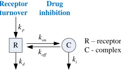
synthesis and degradation, together with drug inhibition as shown schematically in Fig. 1. 99
R – receptor C - complex
p k
d k
on k
off
k C
i k
R Receptor turnover
Drug inhibition
[image:4.595.200.395.234.356.2]100
Fig. 1 Schematic description of receptor turnover and irreversible inhibition 101
In the receptor turnover process, receptor R is synthesized at a constant rate kp, and degrades
102
following a first-order kinetics with a rate constant kd. For the sake of simplicity, feedback 103
mechanisms and subcellular localisation that regulate protein synthesis and stability are not 104
considered in this model. In the drug inhibition process, a drug molecule first binds R 105
reversibly to comprise an intermediate complex C with association and dissociation rates kon
106
and koff, respectively. Note that kon is an apparent rate that depends on drug concentration.
107
The complex C then forms a covalent bound irreversibly at the second step, in a first-order 108
reaction with a rate constant ki. These two processes can be described respectively as follows.
109
Receptor turnover: kp R kd (1)
110
Drug inhibition: R on Ci off
k k
k (2) 111
Based on mass-balance principles, the corresponding ordinary differential equations (ODEs) 112
5
d
d d on p off
R
k k R k k C
t (3) 114
d
d on off i
C
k R k k C
t (4) 115
with the following units: nM for R, C; nM∙min-1 for kp; and min-1 for kd, kon, koff and ki.
116
Here kp and kd are cell parameters associated to receptor turnover; kon, koff and ki are drug 117
parameters for covalent inhibition process. 118
In the absence of drug, the receptor has a steady state at R0 kp kd nM. Scaling R and C 119
with R0 in (3) and (4), the two concentration variables become dimensionless terms 120
0 d p
rR R R k k and cC R0 C k kd p, respectively, and the ODE model can then be 121
written as 122
d
d d on d off
r
k k r k k c
t (5) 123
d
d on off i
c
k r k k c
t (6) 124
In this dimension-free representation, the initial conditions are set to be r0 r
0 1 and 125
0 0 0c c . We further use koff to scale the time term by k toff , and also to scale 126
reaction rates with on kon koff , i k ki off , and d kd koff . This brings the following 127
two ODEs for dimensionless r and c, respectively: 128
d
d on d d
r
r c
(7) 129
d
1
d on i
c
r c
(8) 130
Denoting X
r c
T, this ODE model can be written in a matrix format 131
0 d 1 d 1 d 0 d with (0)on d d
on i
r
r r
c c c
X
AX f X X
6
where
1
1
on d
on i
A is the state matrix for this linear-time-invariant (LTI) 133
system; f
d 0
T is the nonhomogeneous part; X0
1 0
T is the vector of initial states 134for X. 135
At the steady state when dr d 0 and dc d 0, the steady-state values for r and c are 136
derived from (9) to give 137
1 1
i d ss
i d on i
r
(10) 138
1
on d ss
i d on i
c
(11) 139
Here rss and css are used to denote steady-state values or equilibrium points for r and c, 140
respectively, when time approaches infinity. 141
Note after the above re-scaling, all terms in (9) are dimensionless including concentration 142
variables r and c; time ; and parameters on , i , and d . The ‘disappeared’ receptor 143
synthesis rate kp is included in d through scaling of d kd koff kp
k Roff 0
. Clearly this 144choice of non-dimensionalization requires that koff 0 and kp0 . All variables and 145
parameters in (9) are associated with physical quantities and therefore must be nonnegative. 146
With this dimensionless model, the analysis of system behaviour under different parametric 147
regimes can be conveniently discussed in a unified scheme. 148
3 Fast drug process relative to receptor turnover 149
The parametric regimes have been divided into that of fast drug process and slow drug 150
process. In this section, the process of fast drug binding and dissociation is firstly discussed. 151
3.1 Fast drug binding and dissociation relative to receptor turnover 152
This parametric regime is defined by koff kd and kon kd. In this case, the receptor 153
7
(a) When koff kd, i.e., d 1, the period of target coverage (characterized by 1 koff )
155
is much shorter than that of receptor degradation (characterized by 1kd ), which can 156
be due to: i) short target coverage; ii) slow receptor degradation; and iii) combination 157
of i) and ii). 158
(b) When kon kd, i.e., on d, a receptor binds a drug molecule at a rate much faster 159
than its degradation. 160
Under these two conditions, the term of d can be ignored, and model (9) is approximated by 161
1 1
on
on i
r r
c c (12) 162
Model (12) is actually an ODE model for the cell-free assay with only the drug process in (2) 163
considered. 164
When i 0, by taking dr d 0 and dc d 0, the steady-state of dynamic system 165
(12) is deduced to be 166
0
ss ss
r c (13) 167
How small does kd have to be in comparison to koff and kon so as to ensure the validity 168
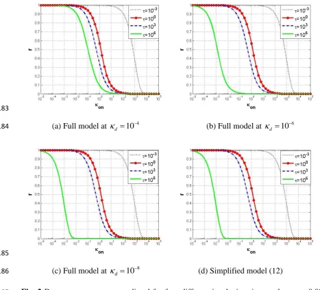
of this approximation? This is examined by the following numerical simulation. Firstly, the 169
full model in (9) is simulated with i 0.001 (koff ki) at three different levels of d:
170
4 10
d
(Fig. 2 (a)); d 106 (Fig. 2 (b)); and d 108 (Fig. 2 (c)). Then the full model is 171
simulated by taking d 0, which is equivalent to the reduced model in (12), using identical 172
value for i , as shown in Fig. 2 (d). The range of on is set to be [1e-5, 1e5] in all 173
simulations. Four incubation time periods are chosen which are separated with an order of 3 174
in time scale between each two, i.e., 10-3, 1, 103 and 106. Comparing simulation results across 175
the four panels in the semi-log Fig. 2, it can be observed that there is a clear difference in 176
dose response in both Fig. 2 (a) and Fig. 2 (b) when compared with the simplified model 177
results in Fig. 2 (d), but the dose response in Fig. 2 (c) is almost the same as that in Fig. 2 (d). 178
This shows that, when d 108, model (12) provides a close approximation for dose 179
8
In all simulation and illustrative results in this paper, the time terms are represented in τ 181
(time t scaled by koff), and the x-axis for on is in log10 scale in dose-response curves.
182
183
(a) Full model at d 104 (b) Full model at d 106 184
185
(c) Full model at d 108 (d) Simplified model (12) 186
Fig. 2 Dose response curves predicted for four different incubation times, when i 0.001. 187
Incubation times shown in the figure legend: black dotted line for 10-3; red line with circles 188
for 100; blue dash-dot line for 103; green solid line for 106. (a) Full model (9) simulated at 189
4 10
d
; (b) Full model simulated at d 106; (c) Full model simulated at d 108; (d) 190
Approximate model in (12). 191
The approximate model in (12) represents a homogeneous LTI system with 192
1 1
on
on i
A . We can use the eigenvalue method to analyse its dynamic 193
[image:8.595.41.509.130.554.2]9
trace( ) 1
A on i
T , det( )A on i, the eigenvalues of A are calculated by
195
2
1,2 T T 4 2
.
196
For the first eigenvalue 197
21
1 1
1 1 4 ,
2 on i 2 on i on i
(14) 198
its associated eigenvector is 199
T 2
T 1 11 21
1 1 4
1 .
2
i on on i on i
on
v v
(15) 200
For the second eigenvalue 201
22
1 1
1 1 4 ,
2 on i 2 on i on i
(16) 202
its associated eigenvector is 203
T 2
T 2 12 22
1 1 4
1 .
2
i on on i on i
on
v v
(17) 204
With initial conditions 𝑟0 = 1 and 𝑐0 = 0, a general analytical solution for (12) can be 205
succinctly written as 206
1 2
1 2
11 12
11 12
( ) 1
( )
( )
r e e
c e e
M (18) 207
where all terms regarding eigenvalues and entries in eigenvectors are provided in (14) - (17). 208
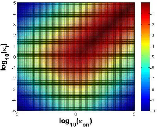
The log10 transformed ratio of the two eigenvalues for different pairs of (on , i ) is
209
plotted in a heat map as shown in Fig. 3. From this diagram it is evident that when the two 210
parameters have similar values and are both above 1, the two eigenvalues 1 and2 are close 211
to each other (the red area in Fig. 3). However, if only one parameter is much larger than 1 or 212
both parameters are much smaller than 1, then the two eigenvalues are widely apart from 213
each other, i.e. 2/ 1 1 (the blue area in Fig. 3), and the time response of the system is 214
10 216
Fig. 3 log (10 2 / 1) plotted as a function of log (10 on) and log ( )10 i . Values between -10 217
and 0 are colour-coded. 218
I II III
219
Fig. 4 Time responses of r and c under on 1, i 0.001 and d 0. 220
For example, when on 1 , i 0.001 , from (14) to (17), the eigenvalues and 221
eigenvectors can be calculated as: 1 2.005, 2 5 104, 1
0.7069 0.7069
T and 222
T2 0.7073 0.7069
. The short-term time response is driven by 1 (see region I in Fig. 223
4), and the long-term time response is driven by 2 (see region III in Fig. 4). Interestingly, 224
between these two regions, both r and c have relatively small variations (see region II in Fig. 225
4). Hence, corresponding dose responses simulated for observation times in this shadowed 226
region would appear to be similar using experimental data. This time-independent 227
[image:10.595.183.399.363.534.2]11
3.2 Fast drug binding/dissociation and fast covalent modification 229
The parametric regime for this scenario is classified by: on d , off d , and
230
i on
, therefore i d. In this case, both reversible binding/dissociation and irreversible
231
modification are much faster than receptor turnover. The system can also be modelled by (12). 232
It can be seen from the heat map in Fig. 3 that the two eigenvalues are close to each other in 233
this region, which means the two inherent time scales are not far away from each other. For 234
the simulations demonstrated in Fig. 5, the two eigenvalues are 1 2.618 and 2 0.382, 235
calculated from (14) and (16), respectively. In this case, the dose response curves measured at 236
different incubation times are predicted to be clearly separated from each other (Fig. 5 (a)). 237
The concentrations of R and C reach steady states with both values at 0 (Fig. 5 (b)), which 238
is consistent with the steady-state analysis conclusion given in (13). Similar to the simulation 239
results shown in Fig. 4, Fig. 5 (b) also demonstrates that the receptor concentration decreases 240
monotonically to its steady state, but the complex concentration goes through a rapid increase 241
initially and then decreases in a slower time scale to its steady state. 242
243
[image:11.595.75.506.407.585.2](a) Dose response curves (b) Time responses under on 1 244
Fig. 5 Dose response curves and time responses of r and c under d 0, on i 1. 245
3.3 Fast drug binding/dissociation and slow covalent modification 246
Under the condition of fast drug process over receptor turnover (koff kd and kon kd), 247
we further consider the regime of koff ki, i.e., i 1. This means the drug dissociation is 248
much faster than the covalent modification. It corresponds to the region in lower part of the 249
12
relatively large energy barrier to covalently modify the receptor; ii) drug dissociation is rapid; 251
iii) a combination of both. Within the parametric region of on d, d 1 and i 1, 252
model (12) can be further reduced to 253
1 1
on on
r r
c c (19) 254
Model (19) is a description for protein-based assay when reversible inhibitor is applied 255
while the covalent modification is negligible. In order to determine how small i should be 256
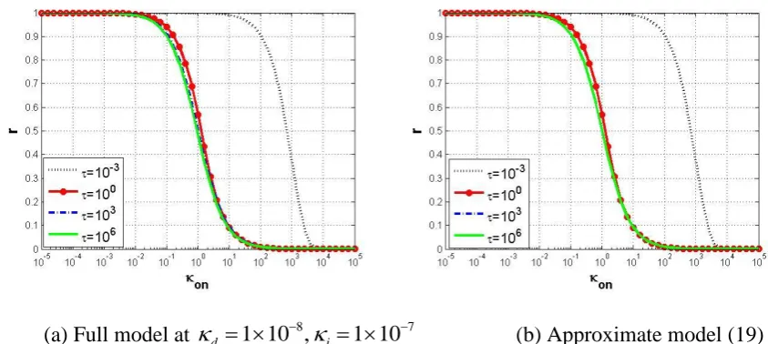
so that the simplified model in (19) can be applied, simulations are conducted using the full 257
model under d 10 ,8 and reduce i gradually to search for the threshold level that will
258
produce a response close to the simplified model response. Fig. 6 shows that when i is 259
reduced to 7
1 10 , the full-model response is very close to that of the simplified model (19). 260
This suggests that when i 10 ,7 the simplified model in (19) can be used to approximate 261
model (12) with a good accuracy. 262
263
(a) Full model at d 1 10 ,8 i 1 107 (b) Approximate model (19) 264
Fig. 6 Dose response curves predicted for different incubation times in : black dotted line 265
for 10-3; red line with circles for 100; blue dash-dot line for 103; green solid line for 106. (a) 266
Full model (9) simulated at d 1 10 ,8 i 1 107; (b) Approximate model in (19). 267
In this case, d d
d d
r c
, T trace( )A
1 on
, det( )A 0, 1 T (on1) and268
2 0
. Under the given initial conditions, the time responses of the two dimensionless 269
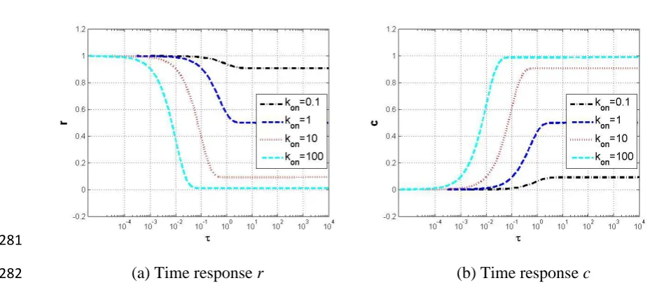
[image:12.595.78.500.395.584.2]13
1 1 1( ) 1
1
( ) 1
1 on on on on on on r e c e (20) 271
The time scale of this dynamic system is determined by 1 or by on. The larger is on, the
272
faster response the system has, and vice versa. The time responses of r and c under different 273
levels of on are illustrated in Fig. 7. 274
With model (19), the steady state is not determined by (13) since i is taken to be zero. In 275
fact, the equilibrium points for system (19) can be derived from (20) to give 276
1 1 1 1 lim 1 1 1 lim 1 1 1 on on ss on on on on on ss on on r e c e (21) 277It can be concluded that rsscss 1 at the steady state. The larger is on, the smaller is rss 278
and the larger is css. This can be clearly seen in the dynamic simulation results shown in Fig. 279
7. 280
281
[image:13.595.38.504.437.654.2](a) Time response r (b) Time response c 282
Fig. 7 Time responses of r and c with approximate model (19) under different levels of on.
283
For incubation time m 1 1
on
, r is close to its steady state (see simulation for each284
on in Fig. 7). Hence, dose response measurements taken beyond this point would appear 285
14
In summary, our analysis of fast drug process suggests for dose response to appear time-287
invariant, the following two requirements need to be satisfied. Firstly, the apparent first-order 288
rate on and the first-order covalent bond formation rate i need to be largely different so 289
that the two time scales characterized by 1 1 and 1 2 are well separated from each other. 290
Secondly, observation time has to be between the two time scales, which corresponds to 291
region II in Fig. 4. It can also be observed from dynamic study that the receptor concentration 292
always decreases monotonically to a steady-state level of zero for the fast drug process, while 293
the concentration of complex C increases rapidly first and then decreases gradually to zero 294
except for the case when covalent modification to complex C is negligible, i.e. i 0. 295
4 Slow drug process relative to receptor turnover 296
In the parametric regime where koff kd or koff kd , i.e. d 1 or d 1 , target 297
coverage duration is comparable to or longer than the receptor life time. This can happen due 298
to: i) long period of target coverage; ii) fast receptor degradation; and iii) combination of both. 299
This might be biologically relevant when receptor homeostasis is tightly regulated at the 300
turnover level. The full model in (9) is used in this regime. 301
Again the eigenvalue method can be used to analyze the system dynamics. The 302
homogeneous part of (9) is XAX. The trace of A is T trace( )A
1 ond i
, 303the determinant of A is det( )A d on i d i . The two eigenvalues are
304
2
1,2 1
4
2 T T
.
305
For 1 1
2 4
2 T T
, the associated eigenvector is 306
T 2
T 1 11 21
1 1 4
1 .
2
i on d i on d on
on
v v
307
For 2 1
2 4
2 T T
, the associated eigenvector is 308
T 2
T 2 12 22
1 1 4
1 .
2
i on d i on d on
on
v v
15
Under the initial condition of X0
1 0
T, the general solution to the homogeneous part 310can be written as M( ) in (18). Taking the non-homogeneous part f
d 0
T into account, 311the general solution to (9) is written as follows 312
T 1 10 0
( ) ( ) ( ) (0) ( ) ( ) ( ) d
r c M M X M
M t f t t (22) 313The steady-state values of r and c can be obtained through numerical integration with (22), or 314
calculated explicitly by (10) and (11). 315
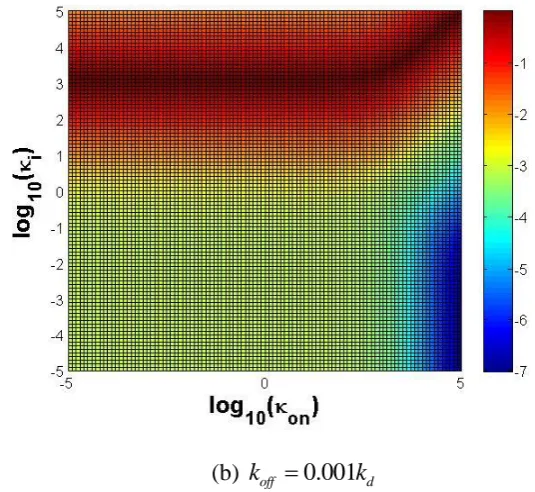
Similar to the heat map in Fig. 3, we first plot log (10 2/ 1) as a function of on and i 316
in log10 scales (Fig. 8). Taking koff kd , i.e. d 1 (Fig. 8 (a)), separation of time scales
317
happens if either kon koff and ki koff (blue region in Fig. 8 (a)), or kon koff and 318
i off
k k (light green region in Fig. 8 (a)), with the former leads to more pronounced effects. 319
In contrast, in the case of koff 0.001kd, i.e. d 1000 (Fig. 8 (b)), separation of time scales 320
takes place if ki koff (bottom part in Fig. 8 (b)), and the condition of kon koff makes the 321
separation more pronounced. 322
323
16 325
[image:16.595.151.419.84.330.2](b) koff 0.001kd 326
Fig. 8 log (10 2 / 1) plotted as a function of log (10 on) and log ( )10 i . Values between -10
327
and 0 are colour-coded. (a) koff kd; (b) koff 0.001kd. 328
The following can be verified in this parametric regime: v11 2
d 1
0 , 32912 1( d 2) 0
v . Considering the analytic solution, it is likely for r to decrease first with a 330
time scale determined by 1 and then recover with a time scale determined by 2 in the 331
longer term, if 1 and 2 are sufficiently apart. 332
An example is discussed to illustrate these ideas by taking koff kd and ki kd. This 333
means the receptor degradation is as fast as target coverage and the drug overcomes a large 334
energy barrier to covalently modify the receptor. 335
Suppose koff kd and ki 0.001kd. Under this condition, receptor initially decreases as a 336
result of drug inhibition, and then recovers towards steady states (see Fig. 9 (c) and Fig. 9 (d)). 337
In the context of dose response curves, this means measurement taken before recovery in r 338
would make the drug appear more potent than the actual steady-state response. For on 1, r 339
is predicted to be smaller for 1 than for 10, 100, 1000 (Fig. 9 (a)). In addition, this 340
trend is consistent throughout on values to a larger range (Fig. 9 (b)). Hence, the dose 341
response simulated for 1(black dotted curve) appears to be more potent than any other 342
17 344
[image:17.595.46.511.81.488.2](a) 3 [1, 10 ]
(b) 6 [1, 10 ]
345
346
(c) on d 1 (d) on 10,d 1 347
Fig. 9 Dose response curves, time response of r and c under i 0.001. 348
According to the heat map in Fig. 8 (a), higher on leads to smaller 2 (the blue region in 349
Fig. 8 (a)), which makes recovery time in r being longer. To examine this observation, time 350
responses of r and c are simulated for on 1 and on10, respectively, as shown in Fig. 9 351
(c) and (d). It can be seen that time response simulation at on10 predicts an elongated 352
recovery period in r (Fig. 9 (d)) compared with that in on 1 (Fig. 9 (c)). This observation is 353
consistent with the separation of different dose response curves in Fig. 9 (a). 354
In slow drug process, the increase of complex concentration is monotonic over time, while 355
the receptor concentration first decreases in a short time and then increase towards a constant 356
level in a longer time. The numerical solutions for r and c at steady states shown in Fig. 9 (c) 357
and (d) are validated by the model-based analytical results in (10) and (11). 358
18 5 Applications
360
Aberrant activity in Epidermal Growth Factor Receptor (EGFR) signaling has profound 361
implications in different types of tumour. Recently, koff kon and ki are reliably quantified
362
from cell-free assays for different irreversible EGFR mutant (EGFRm) inhibitors [20]. 363
However, this study was not able to determine the actual values of *
on kon afatinib koff
364
and koff. Instead, kon*, that is kon
drug
in our context, was assumed to be close to diffusion 365limit at 100µM-1s-1 in order to calculate values for koff. The reported values are tabulated 366
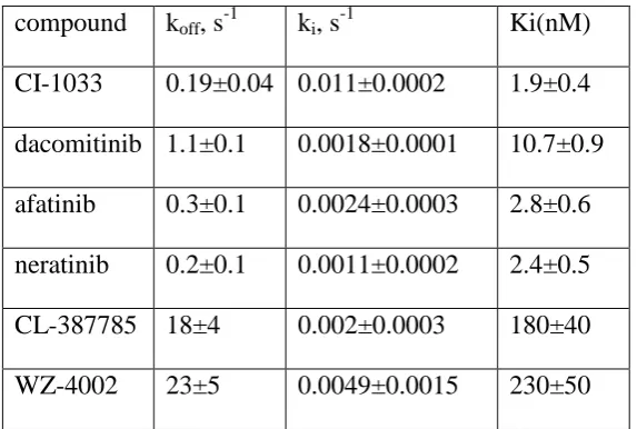
below: 367
compound koff, s-1 ki, s-1 Ki(nM)
[image:18.595.103.390.283.476.2]CI-1033 0.19±0.04 0.011±0.0002 1.9±0.4 dacomitinib 1.1±0.1 0.0018±0.0001 10.7±0.9 afatinib 0.3±0.1 0.0024±0.0003 2.8±0.6 neratinib 0.2±0.1 0.0011±0.0002 2.4±0.5 CL-387785 18±4 0.002±0.0003 180±40 WZ-4002 23±5 0.0049±0.0015 230±50
Table 1. Parameter values inferred from reaction progress curves measured for H1975 cells 368
carrying L858R and T790M mutations in EGFR, using an ODE model. This table is 369
reproduced from the supplementary information in [20]. The plus-or-minus values are 370
standard deviations from averaging three replicated, entirely independent experiments. 371
i on off
K k k . 372
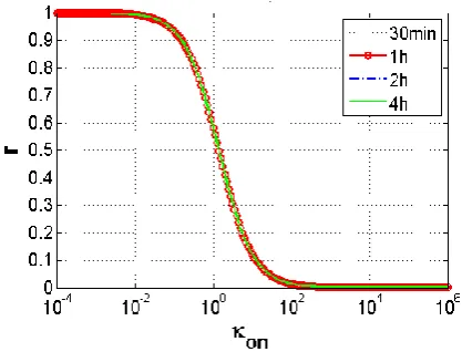
We simulated the cell-free assay of afatinib by using the model in (9) by taking d 0. This 373
predicts the IC50 for on at 30-minutes incubation has a mean value of 0.13 (i.e. assuming
374
3 1 2.4 10 s
i
k , 1
0.3s
off
k ) (see Fig. 10 (a)). Since *
] [
on kon afatinib koff
, afatinib’s
375
IC50 at 30-minutes incubation is predicted to be 0.4nM. Considering different combinations
376
of ki and koff values as reported in Table 1, afatinib’s IC50 at 30-minute incubation is
377
19
It is reported that the internalisation rate of EGFR receptor is approximately 0.2min-1 in 379
breast cancer cells [21]. Hence, d kd koff 1.1 10 2. Considering i 8.0 10 3, this is 380
similar to the fast drug process parametric regime discussed in Section 3.3. Model simulation 381
in Fig. 6 suggests dose response curves taken at 1 and 100 should be close. 382
Using model (12) to mimic in vitro cell assay conditions by taking d 1.1 10 , 2 simulated 383
dose response curves at different incubation durations shift further to right (Fig. 10 (b)) 384
compared with that of d 0 (Fig. 10 (a)). In Fig. 10 (b), with IC50 for on at 1-hour
385
incubation at approximately 1.4, a 10-fold increase from the predicted protein-based assay 386
(i.e. 0.13) is observed. Consistent with these simulation results, approximately 10-fold 387
difference was reported forcell-based assay and protein-based assay for afatinib [21] 388
It can be seen from the above discussions that the simple model in (9) can be used 389
conveniently to generate insights into the connections and differences between protein-based 390
assay and cell-based assay. 391
392
(a) d 0, i 8.0 10 3. This mimics (b) d 1.1 10 2, i 8.0 10 3. This 393
[image:19.595.307.516.393.552.2]the cell-free assay condition. mimics the in vitro cell assay. 394
Fig. 10 Simulated dose response curves for afatinib. 395
6. Conclusions and discussions 396
At lead generation and optimization, it is important to understand the Mechanism Of 397
Action (MOA) of a chemical compound, as well as the Structure-Activity Relationship 398
(SAR), in the hope that ultimately a compound with sufficient therapeutic efficacy is taken 399
20
characterisation. This often remains unknown for compounds coming out of empirical 401
screening methods. Towards this goal, assays have been established to study inhibition 402
reversibility [22]. It is generally accepted that response to irreversible inhibitors are time-403
dependent. Hence, it is often taken for granted that time-independence indicates inhibition 404
reversibility. However, our model-based analysis refutes this claim. 405
We demonstrated iff inhibitor binding and dissociation processes are much quicker than 406
receptor turnover, this system can be approximated by one concerning inhibition only, which 407
is equivalent to the protein-based assay. Based on the numerical simulation using a simple 408
model, it is observed that for protein-based assays, under certain parameter conditions, the 409
dose response curves can be very similar to each other (compare the middle curves in Fig. 2 410
(d)), given 1000-fold variation in incubation time. This indicates dose responses might appear 411
time-invariant for a particular parameter setting. In practice, these data might not be 412
statistically different and can be erroneously taken as evidence of reversible inhibitor. 413
We subsequently analyzed the impact of cell parameters on dose response, including target 414
synthesis and degradation, using the proposed model. Our ensuing analysis of the eigenvalues 415
provides a more general understanding. For dose response to appear time-invariant, the 416
apparent first-order association rate on and the first-order covalent bond formation rate i
417
need to be well separated so that the system has two very different time scales. In particular, 418
when a slowly-dissociating irreversible drug is applied to a receptor under fast turnover, dose 419
response may be highly similar to each other under a variety of incubation periods. Hence, it 420
is inappropriate to conclude an inhibitor being reversible given time-independent dose 421
response, either based on protein-based assay or cell-based assay. 422
The main purpose of this analysis is to demonstrate the relationship between dose response 423
and parameter values in drug and cell processes. For the sake of simplicity, we only 424
considered a linear model in which each reaction follows first-order kinetics. In addition, we 425
did not consider biological regulation over synthesis, degradation and sub-cellular 426
localisation of a receptor [20]. Results obtained in this paper are specific to the form of this 427
linear model. In reality, receptors are often regulated under different levels via feedback 428
mechanisms. This often necessitates mechanistic modelling of a biological pathway to aid in 429
interpretation of in vitro cell assays. 430
It is evident from both numerical simulation and analytical study that the proposed model 431
21
the reduced model (12) is proposed. The receptor concentration decreases monotonically to 433
its steady-state level of zero, while the complex concentration initially increases rapidly and 434
then decreases gradually to zero when the complex elimination is considered (see (13) for 435
steady-state calculation). When the complex elimination is negligible, the reduced model (19) 436
is used. The system will have non-zero steady states for both r and c following a conservation 437
law of rsscss 1 (see (21) for the explicit solution). For the slow drug process including 438
both reactions (1) and (2), the full model (9) is used to describe the dynamic system, and the 439
steady-states are explicitly represented by (10) and (11) for r and c, respectively. In this case, 440
the complex concentration increases monotonically over the whole process, but the receptor 441
concentration first decreases rapidly and then increases gradually on a slower time scale back 442
towards its steady state. The similar rebound behaviour in receptor was also observed and 443
discussed in other TMDD model-based studies [12; 14; 15]. 444
For a drug discovery and development programme, the in vitro model should be used to 445
identify parameter values from in vitro data. These parameters can be used subsequently to 446
help identify the remaining parameter values in the in vivo model. This step-wise fitting may 447
reduce uncertainty in parameter estimation. In this context, the in vitro model described in 448
this paper improves the utility of TMDD models. 449
Acknowledgment 450
TY would gratefully acknowledge Hitesh Mistry (University of Manchester), James Yates 451
(AstraZeneca UK Ltd) and Chris Brackley (University of Edinburgh) for useful discussions. 452
HY would like to thank Professor Peter Halling and Mr Hui Yu from the University of 453
Strathclyde for useful discussions and support in Matlab coding. 454
References 455
[1] Sorger, P. K., Allerheiligen, S. R., Abernethy, D. R., et al.: 'Quantitative and systems 456
pharmacology in the post-genomic era: new approaches to discovering drugs and 457
understanding therapeutic mechanisms', NIH Bethesda, An NIH white paper by the 458
QSP workshop group, 2011), 1-48 459
[2] Gibiansky, L. and Gibiansky, E.: 'Target-mediated drug disposition model: 460
approximations, identifiability of model parameters and applications to the population 461
pharmacokinetic and pharmacodynamic modeling of biologics', Expert Opin Drug 462
22
[3] Ma, P.: 'Theoretical considerations of target-mediated drug disposition models: 464
simplifications and approximations', Pharmaceutical research, 2012, 29, (3), 866-882 465
[4] Marathe, A., Krzyzanski, W. and Mager, D. E.: 'Numerical validation and properties of a 466
rapid binding approximation of a target-mediated drug disposition pharmacokinetic 467
model', Journal of Pharmacokinetics and Pharmacodynamics, 2009, 36, (3), 199-219 468
[5] Yan, X., Mager, D. E. and Krzyzanski, W.: 'Selection between Michaelis–Menten and 469
target-mediated drug disposition pharmacokinetic models', Journal of pharmacokinetics 470
and pharmacodynamics, 2010, 37, (1), 25-47 471
[6] Vicini, P.: 'Multiscale modeling in drug discovery and development: future opportunities 472
and present challenges', Clinical Pharmacology & Therapeutics, 2010, 88, (1), 126-129 473
[7] Mager, D. E. and Krzyzanski, W.: 'Quasi-equilibrium pharmacokinetic model for drugs 474
exhibiting target-mediated drug disposition', Pharmaceutical Research, 2005, 22, (10), 475
1589-1596 476
[8] Gibiansky, L. and Gibiansky, E.: 'Target-mediated drug disposition model: relationships 477
with indirect response models and application to population PK–PD analysis', Journal 478
of Pharmacokinetics and Pharmacodynamics, 2009, 36, (4), 341-351 479
[9] Orrell, D. and Fernandez, E.: 'Using predictive mathematical models to optimise the 480
scheduling of anti-cancer drugs', Innovations in Pharmaceutical Technology, 2010, 33, 481
58-62 482
[10] Yankeelov, T. E., Atuegwu, N., Hormuth, D., et al.: 'Clinically relevant modeling of 483
tumor growth and treatment response', Science Translational Medicine, 2013, 5, (187), 484
187ps9-187ps9 485
[11] Bonate, P.: 'What happened to the modeling and simulation revolution?', Clinical 486
Pharmacology & Therapeutics, 2014, 96, (4), 416-417 487
[12] Aston, P. J., Derks, G., Agoram, B. M. and Van Der Graaf, P. H.: 'A mathematical 488
analysis of rebound in a target-mediated drug disposition model: I. Without feedback', 489
Journal of Mathematical Biology, 2014, 68, (6), 1453-1478 490
[13] Peletier, L. A. and Gabrielsson, J.: 'Dynamics of target-mediated drug disposition', 491
European Journal of Pharmaceutical Sciences, 2009, 38, (5), 445-464 492
[14] Peletier, L. A. and Gabrielsson, J.: 'Dynamics of target-mediated drug disposition: 493
characteristic profiles and parameter identification', Journal of Pharmacokinetics and 494
Pharmacodynamics, 2012, 39, (5), 429-451 495
[15] Aston, P. J., Derks, G., Raji, A., Agoram, B. M. and Van Der Graaf, P. H.: 496
23
of monoclonal antibodies: predicting in vivo potency', Journal of theoretical biology, 498
2011, 281, (1), 113-121 499
[16] Strelow, J., Dewe, W., Iversen, P., et al.: 'Mechanism of Action assays for Enzymes', 500
2004, 501
[17] Nagar, S., Jones, J. P. and Korzekwa, K.: 'A numerical method for analysis of in vitro 502
time-dependent inhibition aata. Part 1. theoretical considerations', Drug Metabolism 503
and Disposition, 2014, 42, (9), 1575-1586 504
[18] Copeland, R. A., Pompliano, D. L. and Meek, T. D.: 'Drug–target residence time and its 505
implications for lead optimization', Nature Reviews Drug Discovery, 2006, 5, (9), 730-506
739 507
[19] You, T., Stansfield, I., Romano, M. C., Brown, A. J. and Coghill, G. M.: 'Analysing 508
GCN4 translational control in yeast by stochastic chemical kinetics modelling and 509
simulation', BMC systems biology, 2011, 5, (1), 131 510
[20] Lauffenburger, D. A. and Linderman, J. J. Receptors: models for binding, trafficking, 511
and signaling. Oxford University Press New York:, 1993. 512
[21] Hendriks, B. S., Opresko, L. K., Wiley, H. S. and Lauffenburger, D.: 'Coregulation of 513
Epidermal Growth Factor Receptor/Human Epidermal Growth Factor Receptor 2 514
(HER2) Levels and Locations Quantitative Analysis of HER2 Overexpression Effects', 515
Cancer Research, 2003, 63, (5), 1130-1137 516
[22] Schwartz, P. A., Kuzmic, P., Solowiej, J., et al.: 'Covalent EGFR inhibitor analysis 517
reveals importance of reversible interactions to potency and mechanisms of drug 518
resistance', Proceedings of the National Academy of Sciences, 2014, 111, (1), 173-178 519