The Partially Truncated Euler–Maruyama Method and
its Stability and Boundedness
Qian Guoa, Wei Liua,∗, Xuerong Maob, Rongxian Yuea
aDepartment of Mathematics, Shanghai Normal University, Shanghai, 200234, China. bDepartment of Mathematics and Statistics, University of Strathclyde, Glasgow, G1 1XH,
U.K.
Abstract
The partially truncated Euler–Maruyama (EM) method is proposed in this
pa-per for highly nonlinear stochastic differential equations (SDEs). We will not
only establish the finite-time strong Lr-convergence theory for the partially
truncated EM method, but also demonstrate the real benefit of the method by
showing that the method can preserve the asymptotic stability and boundedness
of the underlying SDEs.
Keywords: Stochastic differential equation, local Lipschitz condition,
Khasminskii-type condition, partially truncated Euler-Maruyama method,
stability
1. Motivation
It is known (see, e.g., [13, 16, 17]) that the scalar stochastic differential
equation (SDE)
dx(t) =− x(t) +x5(t)
dt+x2(t)dB(t), t≥0, (1.1)
is exponentially stable in the mean square sense, whereB(t) is a scalar Brownian
motion. More precisely, the solution satisfies
E|x(t)|2≤ |x0|2e−
15t
8 , t≥0, (1.2)
∗Corresponding author
for any initial valuex(0) =x0 ∈R(see Example 4.4 below). It is also known
(see, e.g., [9, 11]) that the (classical) Euler–Maruyama (EM) method may not
preserve the exponential stability in the mean square sense (see, e.g., [14, 18]
for the EM method).
Recently, the truncated EM method was developed in [20, 21], where the
finite-time strong convergence theory was established and the order of Lq
-convergence was shown to be arbitrarily close to q/2 for a class of SDEs
in-cluding the underlying SDE (1.1). We therefore wonder if the truncated EM
method can preserve the mean square exponential stability of the underlying
SDE (1.1).
To apply the truncated EM method for a given step size ∆, we need to
truncate the drift coefficientf(x) =−x−x5and the diffusion coefficientg(x) =
x2 into
f∆(x) =f(π∆(x)) and g∆(x) =g(π∆(x)),
where π∆(x) = (|x| ∧µ−1(h(∆)))x/|x| and both functions µ−1 and hwill be explained in the next section. The truncated EM solution is then obtained by
applying the EM method to the truncated SDE
dx(t) =f∆(x(t))dt+g∆(x(t))dB(t).
In other words, the truncated EM solution is formed by settingX0 =x0 and computing
Xk+1=Xk+f∆(Xk)∆ +g∆(Xk)∆Bk, k≥0.
When we try to show if this truncated EM solution is exponentially stable in the
mean square sense for all sufficiently small step size ∆, we note the following
factor: the drift coefficient contains the fifth power term −x5 and the linear term−xwhile the diffusion coefficient contains the square termx2but all these terms are truncated. We realise that it is necessary to truncate the the fifth
power term −x5 and the square term x2; otherwise the EM solution will not converge to the true solution in the moment sense at a finite time (see, e.g.,
fact, from the finite-time-convergence point of view, the linear term does not
cause any problem to the EM method and hence there is no point to truncate
it. Moreover, from the stability point of view, it is this linear term that plays
a key role for the mean square exponential stability of the underlying SDE
(1.1). In other words, truncating the linear term spoils the stability feature of
the underlying SDE (1.1). Based on these observations, we feel it is better to
partially truncate the underlying SDE (1.1) into the following form
dx(t) =−(x(t) + (π∆(x(t)))5)dt+ (π∆(x(t)))2dB(t), (1.3)
and then apply the EM method to this SDE to form the numerical solution:
X0=x0 and
Xk+1 =Xk−(Xk+ (π∆(Xk))5)∆ + (π∆(Xk))2∆Bk, k≥0. (1.4)
We shall see that this numerical solution does not only converge to the true
solution at a finite time but it is also exponentially stable in the mean square
sense for sufficiently small step size ∆. This example motivates us to propose
the the partially truncated EM method in the next section.
It turns out that the partially truncated EM method can preserve the
asymp-totic boundedness of the SDEs. For example, consider the scalar stochastic
Ginzburg–Landau equation (see, e.g., [5, 14])
dx(t) = (ax(t)−bx3(t))dt+cx(t)dB(t), (1.5)
where a, b, c are three positive numbers. It is known (see [22] or Example 5.4
below) that the second moment of the solution of this SDE is asymptotically
bounded. It is also known (see, e.g., [9, 11]) that the EM method may not
preserve this asymptotic boundedness. However, we will show that our partially
truncated EM method can preserve this boundedness very well.
It needs to mention that several nice explicit methods have been
devel-oped recently for SDEs with both drift and diffusion coefficients growing
super-linearly. The fully tamed Euler method is developed in [12]. A new explicit
developed in [28] and the strong convergence order of 1/2 is obtained. The
two-step BDF-Maruyama scheme of order 1/2 is proposed in [1]. The
pro-jected Euler scheme that uses a different truncating strategy is developed in
[26]. Some general criteria on the convergence and the asymptotic stability of
numerical methods are discussed in [10, 26, 27].
The convergence of numerical methods in other senses are interesting and
important as well. In [2], the authors propose a new algorithm to approximate
the laws of the solutions to a class of SDEs with irregular coefficients. The
pathwise convergences of numerical methods with constant and adaptive step
sizes for some highly non-linear SDEs are studied in [6] and [24], respectively. It
is also interesting to see if these methods could preserve asymptotic properties
of the underlying SDEs in their corresponding senses.
The main contribution of this paper is to prove that the partially
trun-cated EM method is able to preserve the mean square exponential stability and
asymptotic boundedness of underlying SDEs, both of whose drift and diffusion
coefficients are allowed to grow super-linearly.
Let us begin to develop our partially truncated EM method and demonstrate
its real benefits.
2. The partially truncated EM method
Throughout this paper, unless otherwise specified, we will use the following
notation. IfAis a vector or matrix, its transpose is denoted byAT. Ifx∈
Rd,
then|x|is the Euclidean norm. IfAis a matrix, we let|A|=ptrace(ATA) be
its trace norm. IfAis a symmetric matrix, denote byλmax(A) andλmin(A) its largest and smallest eigenvalue, respectively. For two real numbersaandb, we
usea∨b= max(a, b) anda∧b= min(a, b). IfD is a set, its indicator function
is denoted byID, namelyID(x) = 1 if x∈ D and 0 otherwise. Moreover, let
(Ω,F,P) be a complete probability space with a filtration{Ft}t≥0satisfying the
usual conditions (that is, it is right continuous and increasing whileF0contains
be anm-dimensional Brownian motion defined on the space.
Consider ad-dimensional SDE
dx(t) =f(x(t))dt+g(x(t))dB(t) (2.1)
ont≥0 with the initial valuex(0) =x0∈Rd, where
f :Rd→Rd and g:Rd→Rd×m.
We assume thatf andg can be decomposed as
f(x) =F1(x) +F(x) and g(x) =G1(x) +G(x), (2.2)
whereF1, F :Rd→RdandG1, G:Rd→Rd×m. We also impose three standing
hypotheses.
Assumption 2.1. Assume that the coefficients F1, F, G1, G satisfy the
fol-lowing conditions: there are constantsL1>0 andr≥0 such that
|F1(x)−F1(y)| ∨ |G1(x)−G1(y)| ≤L1|x−y| (2.3)
and
|F(x)−F(y)| ∨ |G(x)−G(y)| ≤L1(1 +|x|γ+|y|γ)|x−y| (2.4)
for allx, y∈Rd.
We can derive from (2.3) that the coefficientsF1 and G1 satisfy the linear growth condition that there exists a constantK1>0 such that
|F1(x)| ∨ |G1(x)| ≤K1(1 +|x|) (2.5)
for allx∈Rd.
Assumption 2.2. Assume that the coefficients F and Gsatisfy the following
condition: there is a pair of constantsr >¯ 2 andL2 such that
(x−y)T(F(x)−F(y)) +r¯−1
2 |G(x)−G(y)|
2≤L2|x−y|2 (2.6)
Assumption 2.3. Assume that the coefficientsF andGsatisfy the
Khasminskii-type condition: there is a pair of constantsp >¯ r¯andK2>0 such that
xTF(x) +p¯−1 2 |G(x)|
2≤K2(1 +|x|2) (2.7)
for allx∈Rd.
Indeed, (2.7) can be indicated by (2.6). But this approach may force ¯pto
be less than ¯r, which is not necessary. We will see it by the example in Section
3.2.
We derive from (2.5) and (2.7) that for anyp∈(2,p¯),
xTf(x) +p−1 2 |g(x)|
2
≤ xT(F1(x) +F(x)) +p−1
2 (|G1(x)|
2+ 2|G1(x)||G(x)|+|G(x)|2)
≤ |x||F1(x)|+xTF(x) +p−1 2
|G1(x)|2+p−1 ¯
p−p|G1(x)|
2+p¯−p
p−1|G(x)|
2+|G(x)|2
= |x||F1(x)|+
(p−1)(¯p−1) 2(¯p−p) |G1(x)|
2+xTF(x) +p¯−1 2 |G(x)|
2
≤ K3(1 +|x|2), (2.8)
where
K3= 2K1+K2+
K12(p−1)(¯p−1) ¯
p−p .
In a similar manner, we can derive from (2.3) and (2.6) that for anyr∈(2,r¯)
(x−y)T(f(x)−f(y)) +r−1
2 |g(x)−g(y)| 2
≤L3|x−y|2, (2.9)
where
L3= 2L1+L2+
L2
1(r−1)(¯r−1) ¯
r−r .
We can therefore state a known result (see, e.g., [18, 25]) as a lemma for the
use of this paper.
Lemma 2.4. Under Assumptions 2.1, 2.2 and 2.3, the SDE (2.1) has a unique
global solutionx(t)and, moreover, for any p∈(2,p¯),
sup 0≤t≤TE
where, and from now on,C stands for generic positive real constants dependent
on T,p, p, K¯ 1,K2, x0 but independent of the step size∆ (and R later) and its
values may change between occurrences.
To define the partially truncated EM numerical solutions, we first choose a
strictly increasing continuous functionµ : R+ → R+ such that µ(r) → ∞ as
r→ ∞and
sup |x|≤r
|F(x)| ∨ |G(x)|
≤µ(r), ∀r≥1. (2.11)
Denote by µ−1 the inverse function of µ and we see that µ−1 is a strictly increasing continuous function from [µ(0),∞) toR+. We also choose a number ∆∗∈(0,1] and a strictly decreasing functionh: (0,∆∗]→(0,∞) such that
h(∆∗)≥µ(1), lim
∆→0h(∆) =∞ and ∆
1/4h(∆)≤1, ∀∆∈(0,1). (2.12)
For a given step size ∆∈(0,1), let us define the mappingπ∆:Rd →Rd by
π∆(x) = (|x| ∧µ−1(h(∆))) x |x|,
where we setx/|x|= 0 whenx= 0. We then define the truncated functions
F∆(x) =F(π∆(x)) and G∆(x) =G(π∆(x)) (2.13)
forx∈Rd. It is easy to see that
|F∆(x)| ∨ |G∆(x)| ≤µ(µ−1(h(∆))) =h(∆) ∀x∈Rd. (2.14)
That is, both truncated functions F∆ and G∆ are bounded. Moreover, these truncated functions preserve the Khasminskii-type condition (2.7) for all ∆∈
(0,∆∗] as shown in [20] and we state it here as a lemma for the use of this paper.
Lemma 2.5. Let Assumption 2.3 hold. Then, for all∆∈(0,∆∗], we have
xTF∆(x) + ¯
p−1
2 |G∆(x)| 2
≤2K2(1 +|x|2), ∀x∈Rd. (2.15)
In the same way as (2.8) was proved, we can show that for anyp∈(2,p¯),
xT(F1(x) +F∆(x)) +p−1
2 |G1(x) +G∆(x)|
for allx∈Rd, where
K4= 2K1+ 2K2+
K2
1(p−1)(¯p−1) ¯
p−p .
The discrete-time partially truncated EM numerical solutions X∆(tk) ≈
x(tk) fortk=k∆ are formed by setting X∆(0) =x0 and computing
X∆(tk+1) =X∆(tk)+[F1(X∆(tk))+F∆(X∆(tk))]∆+[G1(X∆(tk))+G∆(X∆(tk))]∆Bk, (2.17)
fork= 0,1,· · ·, where ∆Bk =B(tk+1)−B(tk). There are two versions of the
continuous-time truncated EM solutions. The first one is defined by
¯
x∆(t) = ∞
X
k=0
X∆(tk)I[tk,tk+1)(t), t≥0. (2.18)
This is a simple step process so its sample paths are not continuous. We will
refer this as the continuous-time step-process partially truncated EM solution.
The other one is defined by
x∆(t) =x0+
Z t
0
[F1(¯x∆(s)) +F∆(¯x∆(s))]ds+
Z t
0
[G1(¯x∆(s)) +G∆(¯x∆(s))]dB(s) (2.19)
fort≥0. We will refer this as the continuous-time continuous-sample partially
truncated EM solution. We observe that x∆(tk) = ¯x∆(tk) = X∆(tk) for all
k≥0. Moreover,x∆(t) is an Itˆo process with its Itˆo differential
dx∆(t) = [F1(¯x∆(t)) +F∆(¯x∆(t))]dt+ [G1(¯x∆(t)) +G∆(¯x∆(t))]dB(t). (2.20)
3. Finite-TimeLr-Convergence
This section is divided into two parts. The theoretical results of the strong
convergence are proved in the first subsection and a manual of the method is
presented in the second one.
3.1. Theoretical Results
In this part, we will fix T >0 arbitrarily. The following theorem shows the
Theorem 3.1. Let Assumptions 2.1, 2.2 and 2.3 hold. If p >r,¯ 2p >rγ¯ and
for anyr∈[2,r¯)
h(∆)≥µ((∆r/2(h(∆))r)−1/(p−r)), (3.1)
then there is a∆¯ ∈(0,∆∗] such that for all∆∈(0,∆]¯
E|x∆(T)−x(T)|r≤C∆r/2(h(∆))r (3.2)
and
E|¯x∆(T)−x(T)|r≤C∆r/2(h(∆))r. (3.3)
We will prove this theorem in a similar fashion as [21, Theorem 3.8], so we
need to establish a number of lemmas as in [21].
Lemma 3.2. Let Assumptions 2.1, 2.2 and 2.3 hold and letp∈(2,p¯)be
arbi-trary. Then
sup 0<∆≤∆∗
sup 0≤t≤TE
|x∆(t)|p≤C. (3.4)
Proof. Fix any ∆∈(0,∆∗]. By the Itˆo formula, we derive from (2.19) that, for 0≤t≤T,
E|x∆(t)|p− |x0|p
≤ E Z t
0
p|x∆(s)|p−2xT∆(s)[F1(¯x∆(s)) +F∆(¯x∆(s))] +p−1
2 |G1(¯x∆(s)) +G∆(¯x∆(s))| 2ds
= E Z t
0
p|x∆(s)|p−2x¯T∆(s)[F1(¯x∆(s)) +F∆(¯x∆(s))] +
p−1
2 |G1(¯x∆(s)) +G∆(¯x∆(s))| 2ds
+ E
Z t
0
p|x∆(s)|p−2(x∆(s)−x¯∆(s))T[F1(¯x∆(s)) +F∆(¯x∆(s))]ds. (3.5)
By (2.16), we then have
E|x∆(t)|p− |x0|p≤J1+J2+J3, (3.6)
where
J1=E Z t
0
pK4|x∆(s)|p−2(1 +|¯x∆(s)|2)ds, (3.7)
J2=E Z t
0
and
J3=E Z t
0
p|x∆(s)|p−2|x∆(s)−x¯∆(s)||F∆(¯x∆(s))|ds. (3.9)
By the Young inequalityaβb1−β≤βa+ (1−β)bfor a, b≥0 andβ ∈(0,1) as well as the elementary inequality|x|p−2≤1 +|x|p, we can show easily that
J1≤C
1 +
Z t
0
(E|x∆(s)|p+E|¯x∆(s)|p)ds
. (3.10)
Similarly, by Assumption 2.1, we can show that
J2≤C
1 +
Z t
0
(E|x∆(s)|p+E|¯x∆(s)|p)ds
. (3.11)
Moreover, by the Young inequality and (2.14), we derive
J3 ≤ (p−2)E Z t
0
|x∆(s)|pds+ 2
E Z t
0
|x∆(s)−x¯∆(s)|p/2|F∆(¯x∆(s))|p/2ds
≤ (p−2)
Z t
0
E|x∆(s)|pds+ 2(h(∆))p/2
Z t
0
E|x∆(s)−x¯∆(s)|p/2ds.(3.12)
On the other hand, for any s ∈ [0, T], there is a unique k ≥ 0 such that
tk ≤s≤tk+1. By Assumption 2.1, (2.14) and the properties of the Itˆo integral
(see, e.g., [18]), we then derive from (2.19) that
E|x∆(s)−x¯∆(s)|p/2=E|x∆(s)−x∆(tk)|p/2
= E
Z s
tk
[F1(¯x∆(tk)) +F∆(¯x∆(tk))]du+
Z t
tk
[G1(¯x∆(tk)) +G∆(¯x∆(tk))]dB(u)
p/2
≤ C∆p/41 +E|¯x∆(tk)|p/2+ (h(∆))p/2
= C∆p/41 +E|¯x∆(s)|p/2+ (h(∆))p/2
. (3.13)
Substituting this into (3.12) and recalling (2.12), we get
J3 ≤ (p−2)
Z t
0
E|x∆(s)|pds+ 2C(h(∆))p/2∆p/4 Z t
0
1 +E|¯x∆(s)|p/2+ (h(∆))p/2ds
≤ C1 +
Z t
0
(E|x∆(s)|p+E|¯x∆(s)|p)ds
. (3.14)
Substituting (3.10), (3.11) and (3.14) into (3.6), we have
E|x∆(t)|p ≤ C
1 + Z t 0 sup 0≤u≤sE
|x∆(u)|pds
As this holds for anyt∈[0, T] while the right-hand side is non-decreasing int,
we then see
sup 0≤u≤tE
|x∆(u)|p≤C1 +
Z t
0 sup 0≤u≤sE
|x∆(u)|pds.
The well-known Gronwall inequality yields that
sup 0≤u≤TE
|x∆(u)|p≤C.
As this holds for any ∆ ∈ (0,∆∗] while C is independent of ∆, we see the required assertion (3.4). 2
The following lemma shows that x∆(t) and ¯x∆(t) are close to each other in the sense ofLp.
Lemma 3.3. Let Assumptions 2.1, 2.2 and 2.3 hold and letp∈(2,p¯)be
arbi-trary. Then there is a∆¯ ∈(0,∆∗]such that for all ∆∈(0,∆]¯ ,
E|x∆(t)−x¯∆(t)|p≤C∆p/2(h(∆))p, ∀t∈[0, T]. (3.15)
Consequently
lim
∆→0E|x∆(t)−x¯∆(t)|
p= 0. (3.16)
Proof. By Lemma 3.2, there is a ¯∆∈(0,∆∗] such that
sup 0<∆≤∆¯
sup 0≤t≤TE
|x∆(t)|p≤C. (3.17)
Now, fix any ∆∈(0,∆]. For any¯ t ∈[0, T], there is a uniquek≥0 such that
tk ≤t≤tk+1. In the same way as (3.13) was proved, we can then show
E|x∆(t)−x¯∆(t)|p≤C∆p/2
1 +E|¯x∆(t)|p+ (h(∆))p
.
By (3.17), we therefore have
E|x∆(t)−x¯∆(t)|p≤C∆p/2(h(∆))p,
which is (3.15). Noting from (2.12) that ∆p/2(h(∆))p≤∆p/4, we obtain (3.16)
from (3.15) immediately. 2
Lemma 3.4. Let Assumptions 2.1, 2.2 and 2.3 hold. For any real number
R >|x0|, define the stopping time
τR= inf{t≥0 :|x(t)| ≥R},
where throughout this paper we setinf∅=∞(and as usual∅ denotes the empty
set). Then
P(τR≤T)≤
C
Rp. (3.18)
(Recall thatC stands for generic positive real constants independent of∆ and
R.)
The following lemma can be proved in the same way as [20, Lemma 3.4] was
proved.
Lemma 3.5. Let Assumptions 2.1, 2.2 and 2.3 hold. For any real number
R >|x0| and ∆ ∈(0,∆]¯ (the same ∆¯ as in Lemma 3.3), define the stopping time
ρ∆,R= inf{t≥0 :|x∆(t)| ≥R}.
Then
P(ρ∆,R≤T)≤
C
Rp. (3.19)
We can now prove Theorem 3.1. As the proof is in a similar fashion as [20,
Theorem 3.5] was proved so we only highlight the different parts.
Proof of Theorem 3.1.
Let ε >0 be arbitrary. Let τR and ρ∆,R be the same as the definitions in Lemmas 3.4 and 3.5. Set
θ∆,R=τR∧ρ∆,R and e∆(T) =x∆(T)−x(T).
For a sufficiently largeR >|x(0)|, we have that
E|e∆(T)|r=E
|e∆(T)|rI{θ∆,R>T}
+E|e∆(T)|rI{θ∆,R≤T}
. (3.20)
For anyδ >0, using the Young inequality we obtain that
E
|e∆(T)|rI
{θ∆,R≤T}
≤ rδ
pE|e∆(T)|
p+ p−r
Applying Lemmas 2.4 and 3.2, we can see that
E|e∆(T)|p≤2p−1E|x(T)|p+ 2p−1E|x∆(T)|p≤C.
Using Lemmas 3.4 and 3.5, we obtain that
P(θ∆,R≤T)≤P(τR≤T) +P(ρ∆,R≤T)≤
C Rp.
Substituting the two estimates above back into (3.21), and choosingδ= ∆r/2(h(∆))r
andR= (∆r/2(h(∆))r)−1/(p−r) we have that
E
|e∆(T)|rI
{θ∆,R≤T}
≤C∆r/2(h(∆))r. (3.22)
In the same way as the proof of Lemma 3.7 in [21], we can show that
E
|e∆(T∧θ∆,R)|r≤C∆r/2(h(∆))r. (3.23)
By (3.1), we can see that
µ−1(h(∆))≥(∆r/2(h(∆))r)−1/(p−r)=R.
Therefore, substituting (3.22) and (3.23) into (3.20) yields (3.2). In addition,
(3.2) together with Lemma 3.3 indicates (3.3). 2
3.2. A Manual of the Method
We demonstrate the process of implementing the partially truncated EM by
the following example.
Example 3.6. Consider a nonlinear test scalar SDE
dx(t) = (x(t)−x5(t))dt+x2(t)dB(t), t≥0,
with the initial value x(0) = 1. It can be seen that F1(x) = x, F(x) = −x5,
G1(x) = 0 and G(x) =x2.
Assumption 2.1 holds clearly. For Assumption 2.2, it is straightforward to
see that
(x−y)(F(x)−F(y)) +r¯−1
2 |G(x)−G(y)| 2
= (x−y)−(x−y)(x4+x3y+x2y2+xy3+y4)+r¯−1 2 (x+y)
2(x−y)2
=−(x4+x3y+x2y2+xy3+y4) +r¯−1 2 (x+y)
2
|x−y|2.
But
−(x3y+xy3) =−xy(x2+y2)≤0.5(x2+y2)2= 0.5(x4+x4) +x2y2.
Hence
(x−y)(F(x)−F(y)) +r¯−1
2 |G(x)−G(y)| 2
≤
−0.5(x4+y4) +r¯−1 2 (x
2+y2)
|x−y|2
≤
1 + (¯r−1) 2 4
|x−y|2.
In other words, Assumption 2.2 is also fulfilled for any ¯r. Moreover,
xF(x) +p¯−1 2 |G(x)|
2 =
−x6+p¯−1 2 |x
2 |2
= −x2(x2−p¯−1 4 )
2+(¯p−1) 2 16 x
2≤ (¯p−1) 2 16 x
2,
i.e. Assumption 2.3 is satisfied for any ¯p.
Step 2. Chooseµ(·)andh(·)
According to (2.11), we setµ(r) =r5 such that
sup |x|≤r
|F(x)| ∨ |G(x)|
= sup |x|≤r
|x|5∨ |x|2
≤r5, ∀r≥1.
We seth(∆) = ∆−1/10, then all the conditions in (2.12) hold for all ∆∗∈(0,1].1
Step 3. DefineF∆(x)andG∆(x)
1One may notice that the choices of bothµ(·) andh(·) are not unique and we do not know
10−4 10−3 10−3
10−2
Step Size
Error
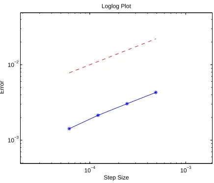
[image:15.612.190.408.126.313.2]Loglog Plot
Figure 1: The strong convergence order at the terminal timeT = 2. The red dashed line is
the reference line with the slope of 1/2.
From Step 2, we can see the truncating factor is defined as µ−1(h(∆)) = ∆−1/50. Then according to (2.13),F
∆(x) andG∆(x) are defined as
F∆(x) =F((|x| ∧∆−1/50)
x
|x|)) and G∆(x) =G((|x| ∧∆
−1/50) x |x|)).
Step 4. Calculation in each iteration
For the given step size ∆ and Xk, we compare |Xk| and ∆−1/50. Then substituting the product of the smaller one and Xk/|Xk| into F(·) and G(·)
yieldsF∆(Xk) andG∆(Xk). TheXk+1 is calculated by
Xk+1=Xk+ (F1(Xk) +F∆(Xk))∆ +G∆(Xk)∆Bk.
Figure 1 displays theL1 errors at the time T = 2 with step sizes 2−14, 2−13, 2−12 and 2−11. The simulations with step size 2−17 are regarded as the true solutions. For each step size, 1000 paths are simulated. Compared with the red
dashed reference line, strong convergence order of the partially truncated
Euler-Maruyama method is approximately 1/2, which is in line with the theoretical
4. Stability
Finite-time convergence is a fundamental property for a numerical method.
However, a nice numerical method for an SDE should also preserve some
asymp-totic properties of the underlying SDE, for example, stability and boundedness
(see, e.g., [4, 8, 9, 15, 19, 23]).
In this section we will show that the partially truncated EM method can
preserve the mean square exponential stability of the underlying SDE (2.1). We
will let Assumptions 2.1–2.3 be the standing hypotheses so we will not mention
them explicitly in the theorems in this section. Moreover, for the stability
purpose, we also assume in this section that
F1(0) =F(0) = 0, G1(0) =G(0) = 0. (4.1)
So the linear growth condition (2.5) becomes
|F1(x)| ∨ |G1(x)| ≤K1|x|. (4.2)
Our main assumption in this section is the following one.
Assumption 4.1. Assume that there are constantsθ∈[0,∞]andλ1> λ2≥0
such that
2xTF1(x) + (1 +θ)|G1(x)|2≤ −λ1|x|2 (4.3)
and
2xTF(x) + (1 +θ−1)|G(x)|2≤λ2|x|2 (4.4)
for all x ∈ Rd, where throughout the remaining part of this paper we choose
θ= 0 and setθ−1|G(x)|2= 0 when there is noG(x)term ing(x), while choose
θ=∞and set θ|G1(x)|2= 0when there is noG1(x)term ing(x).
This assumption implies
2xTf(x) +|g(x)|2≤ −(λ
1−λ2)|x|2, x∈Rd. (4.5)
It is therefore known (see, e.g., [13, 16, 17]) that the SDE (2.1) is exponentially
Theorem 4.2. Let Assumption 4.1 hold. Then for any initial value x0 ∈Rd, the solution of the SDE (2.1) satisfies
E|x(t)|2≤ |x0|2e−(λ1−λ2)t, ∀t≥0. (4.6)
The following theorem shows that the partially truncated EM method can
preserve this mean square exponential stability perfectly.
Theorem 4.3. Let Assumption 4.1 hold. Then for any ε∈(0, λ1−λ2), there
is a∆ˆ ∈(0,∆∗) such that for every∆∈(0,∆)ˆ and any initial valuex0∈Rd, the solution of the partially truncated EM method (2.17) satisfies
E|X∆(tk)|2≤ |x0|2e−(λ1−λ2−ε)tk, ∀k≥0. (4.7)
Proof. To simplify the notation, we define, in the remaining part of this paper,
f∆(x) =F1(x) +F∆(x) and g∆(x) =G1(x) +G∆(x), x∈Rd,
for every ∆∈(0,∆∗]. We first show that these functions preserve property (4.5) perfectly in the sense that
2xTf∆(x) +|g∆(x)|2≤ −(λ
1−λ2)|x|2, x∈Rd. (4.8)
In fact, this holds obviously forx∈Rd with|x| ≤µ−1(h(∆)). Forx∈Rd with
|x|> µ−1(h(∆)), we derive, by Assumption 4.1,
2xTf∆(x) +|g∆(x)|2
≤ 2xTF1(x) + (1 +θ)|G1(x)|2+ 2xTF(π∆(x)) + (1 +θ−1)|G(π∆(x))|2
≤ −λ1|x|2+ 2(x−π∆(x))TF(π∆(x)) + 2(π∆(x))TF(π∆(x)) + (1 +θ−1)|G(π∆(x))|2 ≤ −λ1|x|2+λ2|π∆(x)|2+ 2(x−π∆(x))TF(π∆(x)). (4.9)
But, by Assumption 4.1 again,
Substituting this into (4.9) and noting that|π∆(x)|=µ−1(h(∆)), we get
2xTf∆(x) +|g∆(x)|2≤ −λ1|x|2+λ2|x||π∆(x)| ≤ −(λ
1−λ2)|x|2. (4.10)
Fixx0 ∈Rd arbitrarily. For any ∆∈(0,∆∗], we can easily obtain from (2.17)
that
E|X∆(tk+1)|2 = E
|X∆(tk)|2+|f∆(X∆(tk))|2∆2+|g∆(X∆(tk))∆Bk|2
+ 2X∆(tk)Tf∆(X∆(tk))∆
(4.11)
fork= 0,1,· · ·. But
E(|g∆(X∆(tk))∆Bk|2) = E traceg∆(X∆(tk))∆Bk∆BkTg∆(X∆(tk))T
= E
E traceg∆(X∆(tk))∆Bk∆BkTg∆(X∆(tk))T
Ftk
= Etrace
g∆(X∆(tk))E ∆Bk∆BkT
Ftk
g∆(X∆(tk))T
= Etrace
g∆(X∆(tk))∆Img∆(X∆(tk))T
= ∆E|g∆(X∆(tk))|2,
whereImdenotes them×midentity matrix. Substituting this into (4.11) yields
E|X∆(tk+1)|2 = E
|X∆(tk)|2+|f∆(X∆(tk))|2∆2+|g∆(X∆(tk))|2∆
+ 2X∆(tk)Tf∆(X∆(tk))∆
. (4.12)
Using (4.8), we get
E|X∆(tk+1)|2≤(1−(λ1−λ2)∆)E|X∆(tk)|2+ ∆2E|f∆(X∆(tk))|2. (4.13)
Now, by (4.2), we have
|f∆(x)|2≤2K2 1|x|
2+ 2|F∆(x)|2, ∀x∈
Rd.
But, by (2.4) and (4.1), we have
|F∆(x)|2≤4L2 1|x|
2 if|x| ≤1
while
We hence always have
|f∆(x)|2≤2(K2
1+ 4L21+h2(∆))|x|2, ∀x∈Rd.
Recalling (2.12), we see that for any ε ∈ (0, λ1−λ2), there is a ˆ∆ ∈ (0,∆∗) sufficiently small such that for all ∆∈(0,∆), (ˆ λ1−λ2−ε)∆<1 and
∆|f∆(x)|2≤ε|x|2, ∀x∈Rd. (4.14)
For each such ∆, we hence obtain from (4.13) and (4.14) that
E|X∆(tk+1)|2≤(1−(λ1−λ2−ε)∆)E|X∆(tk)|2≤ |x0|2(1−(λ1−λ2−ε)∆)k+1. (4.15)
By the elementary inequality
1−(λ1−λ2−ε)∆≤e−(λ1−λ2−ε)∆,
we further have
E|X∆(tk+1)|2≤ |x0|2e−(λ1−λ2−ε)tk+1, (4.16) which is the desired assertion (4.7). The proof is complete. 2
Example 4.4. Let us return to the scalar SDE (1.1), namely
dx(t) =−(x(t) +x5(t))dt+x2(t)dB(t), t≥0, (4.17)
with the initial valuex(0) =x0∈R, where B(t) is a scalar Brownian motion.
We decompose the coefficientsf(x) andg(x) in the form of (2.2) with
F1(x) =−x, F(x) =−x5, G1(x) = 0, G(x) =x2
forx∈R. Choosingθ=∞, we then have
2xTF1(x) + (1 +θ)|G1(x)|2=−2|x|2
and
But
−2x6+x4=−2x6−x4+1 8x
2+1 8x
2=−2x2x2−1 4
2
+1 8x
2≤1 8x
2.
In other words, Assumption 4.1 is satisfied with λ1 = 2 and λ2 = 1/8. By Theorem 4.2, the SDE (4.17) is exponentially stable in the mean square sense,
namely, for any initial valuex0∈R, the solution of the SDE (4.17) satisfies
E|x(t)|2≤ |x0|2e−
15t
8 , ∀t≥0. (4.18)
It is also known (see, e.g., [9, 11]) that the EM method might not preserve
this mean square exponential stability. However, our new partially truncated
EM method does preserve this stability perfectly. In fact, it is easy to see that
our standing hypotheses, Assumption 2.1 is satisfied. Assumption 2.2 can be
verified in the same way as that in Example 3.6. Moreover, for any ¯p >2,
xTF(x) +p¯−1 2 |G(x)|
2=−x6+p¯−1 2 x
4
which is bounded above in x ∈ R. In other words, Assumption 2.3 is also
satisfied for any ¯p >2. We can chooseµ(r) =r5 andh(∆) = ∆−1/4 to define the numerical solution X∆(tk) by the partially truncated EM method (2.17). By Theorem 3.1, this numerical solution will converge to the true solution in
Lr for any r ≥ 2 at any finite time. Moreover, by Theorem 4.3, we can also
conclude that for anyε∈(0,15/8), there is a positive number ˆ∆ such that for
every ∆∈(0,∆) and any initial valueˆ x0∈Rd, this numerical solution satisfies
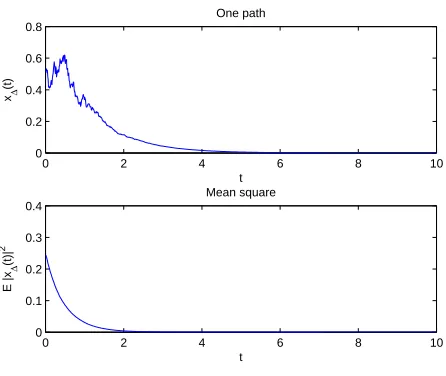
E|X∆(tk)|2≤ |x0|2e−(15/8−ε)tk, ∀k≥0. (4.19) Figure 2 displays the asymptotic behaviour of the equation (4.17). The lower
plot shows that the second moment of the partially truncated Euler-Maruyama
method tends to zero as the time advances. In addition, the behaviour of the
pathwise asymptotic stability can also be observed from the upper plot.
5. Boundedness
Although the stability of numerical methods for SDEs has been studied
0 2 4 6 8 10 0
0.2 0.4 0.6 0.8
One path
t x∆
(t)
0 2 4 6 8 10
0 0.1 0.2 0.3 0.4
Mean square
t
E |x
∆
(t)|
[image:21.612.188.411.127.315.2]2
Figure 2: The upper plot is the simulation of one path and the lower one is the mean square
of 1000 paths.
asymptotic boundedness of numerical methods (see, e.g., [15]).
In this section we will show that the partially truncated EM method can
preserve the asymptotic boundedness of the underlying SDE (2.1). As in the
previous section, we let Assumptions 2.1–2.3 be the standing hypotheses so we
will not mention them explicitly in the theorems in this section. Of course we
will no longer need condition (4.1) and Assumption 4.1 in this section. The
main assumption in this section is the following one.
Assumption 5.1. Assume that there are constants θ∈[0,∞],α1, α2≥0 and
β1> β2≥0 such that
2xTF1(x) + (1 +θ)|G1(x)|2≤α
1−β1|x|2 (5.1)
and
2xTF(x) + (1 +θ−1)|G(x)|2≤α2+β2|x|2 (5.2)
for allx∈Rd.
This assumption implies
2xTf(x) +|g(x)|2≤α
We can hence state a theorem which follows easily from [22, Theorem 5.2 on
page 157].
Theorem 5.2. Let Assumption 5.1 hold. Then for any initial value x0 ∈Rd, the solution of the SDE (2.1) satisfies
lim sup t→∞ E
|x(t)|2≤α1+α2
β1−β2
. (5.4)
The following theorem shows that the partially truncated EM method can
preserve this asymptotic boundedness perfectly.
Theorem 5.3. Let Assumption 5.1 hold. Then for anyε∈(0, β1−β2), there
is a∆ˆ ∈(0,∆∗) such that for every∆∈(0,∆)ˆ and any initial valuex0∈Rd, the solution of the partially truncated EM method (2.17) satisfies
lim sup k→∞ E
|X∆(tk)|2≤ α1+α2+ε
β1−β2−ε
. (5.5)
Proof. Fixε∈(0, λ1−λ2) arbitrarily. We first show that the functionsf∆and
g∆ defined in the previous section preserve property (5.3) almost perfectly in the sense that
2xTf∆(x) +|g∆(x)|2≤α1+α2−(β1−β2−0.5ε)|x|2, x∈Rd, (5.6)
as long as ∆∈(0,∆1), where ˆˆ ∆1∈(0,∆∗) is sufficiently small for which
α2
(µ−1(h( ˆ∆1)))2 ≤0.5ε. (5.7) In fact, fix any ∆∈(0,∆1) and it is obvious that (5.6) holds forˆ x∈Rd with
|x| ≤µ−1(h(∆)). Forx∈Rd with |x|> µ−1(h(∆)), we derive, by Assumption
5.1,
2xTf∆(x) +|g∆(x)|2
≤ 2xTF1(x) + (1 +θ)|G1(x)|2+ 2xTF(π∆(x)) + (1 +θ−1)|G(π∆(x))|2 ≤ α1−β1|x|2+ 2(x−π∆(x))TF(π∆(x))
+ 2(π∆(x))TF(π∆(x)) + (1 +θ−1)|G(π∆(x))|2
But, by Assumption 5.1 again,
2(x−π∆(x))TF(π∆(x)) = 2[|x|/µ−1(h(∆))−1](π∆(x))TF(π∆(x)) ≤ [|x|/µ−1(h(∆))−1]α2+β2(µ−1(h(∆)))2
Substituting this into (5.8) yields
2xTf∆(x) +|g∆(x)|2 ≤ α
1−β1|x|2+ |x|
µ−1(h(∆))
α2+β2(µ−1(h(∆)))2
≤ α1−β1|x|2+α2
|x| µ−1(h(∆))
2
+β2|x|2
≤ α1−(β1−β2−0.5ε)|x|2, (5.9)
where (5.7) have been used. In other words, (5.6) holds for anyx ∈Rd with
|x|> µ−1(h(∆)) too so it holds for allx∈Rdas claimed.
Fixx0∈Rdarbitrarily. For any ∆∈(0,∆1), it follows from (4.12) and (5.6)ˆ
that
E|X∆(tk+1)|2 ≤ ∆(α1+α2) + ∆2E|f∆(X∆(tk))|2
+
1−∆(β1−β2−0.5ε)E|X∆(tk)|2. (5.10)
But, by (2.5) and (2.14),
|f∆(X∆(tk))|2≤2|F1(X∆(t
k))|2+2|F∆(X∆(tk))|2≤4K1(1+|X∆(tk)|2)+2(h(∆))2.
Hence, by (2.12),
∆|f∆(X∆(tk))|2≤4∆K1(1 +|X∆(tk)|2) + 2 √
∆.
Consequently, there is a ˆ∆ ∈ (0,∆ˆ1] sufficiently small such that for any ∆ ∈ (0,∆), ∆(ˆ β1−β2−ε)<1 and
∆|f∆(X∆(tk))|2≤ε+ 0.5ε|X∆(t
k)|2. (5.11)
Now, fix any ∆∈(0,∆). Substituting (5.11) into (5.10) yieldsˆ
E|X∆(tk+1)|2≤∆(α1+α2+ε) +
1−∆(β1−β2−ε)
This implies
E|X∆(tk+1)|2 ≤ ∆(α1+α2+ε)
1 +1−∆(β1−β2−ε)
+
1−∆(β1−β2−ε) 2
E|X∆(tk−1)|2
≤ · · ·
≤ ∆(α1+α2+ε)
1 + k
X
i=1
1−∆(β1−β2−ε) i
+
1−∆(β1−β2−ε)
k+1
|x0|2
= α1+α2+ε
β1−β2−ε
1−
1−∆(β1−β2−ε)
k+1
+
1−∆(β1−β2−ε) k+1
|x0|2. (5.13)
Lettingk→ ∞, we obtain the required assertion (5.5). The proof is complete.
2
Example 5.4. Let us return to the SDE (1.5), namely consider the scalar
stochastic Ginzburg–Landau equation (see, e.g., [5, 14])
dx(t) = (ax(t)−bx3(t))dt+cx(t)dB(t), (5.14)
whereB(t) is a scalar Brownian motion anda, b, care three positive numbers.
We decompose the coefficientsf(x) andg(x) in the form of (2.2) with
F1(x) =−(a+c2)x, F(x) = (2a+c2)x−bx3, G1(x) =cx, G(x) = 0 (5.15)
forx∈R. Choosingθ= 0, we then have
2xF1(x) + (1 +θ)|G1(x)|2=−(2a+c2)x2
and
2xF(x) + (1 +θ−1)|G(x)|2= 2(2a+c2)x2−2bx4≤ (2a+c2)2 2b .
That is, Assumption 5.1 holds with
α1= 0, β1= 2a+c2, α2=
(2a+c2)2
By Theorem 5.2, we then see that for any initial valuex0∈Rd, the solution of
the SDE (5.14) satisfies
lim sup t→∞ E
|x(t)|2≤2a+c2
2b . (5.16)
It is known (see, e.g., [9, 11]) that the EM method may not preserve this
asymp-totic boundedness. However, we now show that our partially truncated EM
method can preserve this boundedness perfectly. In fact, it is easy to see that
the coefficients of the SDE (5.14) with their decompositions in (5.15) satisfy
Assumptions 2.1 - 2.3 for any ¯p > 2. We can choose µ(r) = (2a+c2+b)r3 and h(∆) = ∆−1/4 to define the numerical solution X∆(tk) by the partially truncated EM method (2.17). By Theorem 3.1, this numerical solution will
converge to the true solution inLr for any r≥2 at any finite time. Moreover,
by Theorem 5.3, we can also conclude that for any ε∈(0,2a+c2), there is a positive number ˆ∆ such that for every ∆∈(0,∆) and any initial valueˆ x0∈Rd,
this numerical solution satisfies
lim sup k→∞ E
|X∆(tk)|2≤
(2a+c2)2 2b +ε
2a+c2−ε. (5.17)
Example 5.5. Let us now discuss ad-dimensional SDE
dx(t) =f(x(t))dt+g(x(t))dB(t), (5.18)
ont≥0 with the initial valuex(0) =x0∈Rd. HereB(t) is a scalar Brownian
motion andf, g:Rd→
Rd are defined by
f(x) = diag(x1, x2, ..., xd)(b+Ax2) and g(x) = diag(x1, x2, ..., xd)Cx
forx∈Rd, where b∈Rd,A, C ∈Rd×d andx2= (x21,· · ·, x2d)
T. If we restrict
the state space of this SDE in the positive coneRd
+, it is known as the stochastic power Lotka-Volterra model (see, e.g., [3]). But we here treat this SDE in the
wholeRd-space. Let ¯b= max
1≤i≤d|bi|and decompose the coefficientsf(x) and
g(x) in the form of (2.2) with
and
G1(x) = 0, G(x) = diag(x1, x2, ..., xd)Cx.
It is easy to see that Assumption 2.1 is satisfied. To satisfy Assumption 2.3, we
assume that
−λmax(A+AT)> d λmax(CTC). (5.19)
We then derive that
xTF(x) = ¯b|x|2+ (x2)Tb+ (x2)TAx2≤2¯b|x|2+1
2λmax(A+A T)|x2|2.
But
|x|4= d
X
i,j=1
x2ix2j ≤ d
X
i=1
x4i +1 2
X
i6=j
(x4i +x4j) =d
d
X
i=1
x4i =d|x2|2.
So
xTF(x)≤2¯b|x|2+ 1
2dλmax(A+A
T)|x|4. (5.20)
Moreover,
|G(x)|2=xTCTdiag(x2
1, x22, ..., x2d)Cx≤ |x|2xTCTCx≤λmax(CTC)|x|4. (5.21)
Set
¯
p= 1 + −λmax(A+A T)
dλmax(CTC) . (5.22) We have ¯p >2 by condition (5.19) and, by (5.20) and (5.21),
xTF(x) +p¯−1 2 |G(x)|
2≤2¯b|x|2.
In other words, Assumption 2.3 is satisfied. Let us now verify Assumption 5.1.
Choosingθ=∞, we have
2xTF1(x) + (1 +θ)|G1(x)|2=−2¯b|x|2 (5.23)
and, by (5.20) and (5.21) again,
2xTF(x)+(1+θ−1)|G(x)|2≤4¯b|x|2−1
d
where
α2=
4d¯b2
−λmax(A+AT)−d λmax(CTC). (5.25) That is, Assumption 5.1 is satisfied with
α1= 0, β1= 2¯b, β2= 0 andα2 as defined above.
By Theorem 5.2, we can therefore conclude that under condition (5.19), for any
initial valuex0∈Rd, the solution of the SDE (5.18) satisfies
lim sup t→∞ E
|x(t)|2≤ α2
2¯b. (5.26)
It is known (see, e.g., [9, 11]) that the EM method may not preserve this
asymp-totic boundedness. However, our partially truncated EM method will do. In
fact, We can chooseµ(r) =δr3, for a sufficiently large positive numberδ, and
h(∆) = ∆−1/4 to define the numerical solution X∆(tk) by the partially trun-cated EM method (2.17). By Theorem 3.1, this numerical solution will converge
to the true solution inLr for any 2≤r <p¯at any finite time, where pis
de-fined by (5.22). Moreover, by Theorem 5.3, we can also conclude that for any
ε∈(0,2¯b), there is a positive number ˆ∆ such that for every ∆∈(0,∆) and anyˆ
initial valuex0∈Rd, this numerical solution satisfies
lim sup k→∞ E
|X∆(tk)|2≤ α2+ε
2¯b−ε. (5.27)
6. Discussions and Conclusions
Motivated by two examples discussed in Section 1, we developed a new
ex-plicit numerical scheme, called the partially truncated EM method for nonlinear
SDEs under the local Lipschitz condition plus the Khasminskii-type condition.
We established the finite-time strong Lr-convergence theory for the partially
truncated EM method.
With respect of the finite convergence, we do not claim that our method
also designed for SDEs with both drift and diffusion coefficients growing
super-linearly. Actually, the finite time strong convergence order of those methods
and the partially truncated EM method are 1/2 or arbitrarily close to 1/2.
The real benefits of this new method lie in that the method can preserve the
asymptotic stability and boundedness of the underlying SDEs.
It should be noted that the conditions we imposed to guarantee the mean
square exponential stability and the mean square asymptotic boundedness are
only sufficient, but not necessary. In addition, our assumptions require the
drift coefficient to dominate the diffusion coefficient in the negative direction,
which may exclude some types of SDEs, such as some driftless SDEs with
super-linear diffusion. Therefore, it is interesting to investigate whether the partially
truncated EM method can still work if the assumptions in this paper are further
released.
Acknowledgements
The authors would like to thank all the three referees and the editor for the
very useful comments and suggestions, which have helped to improve the paper
a lot.
The authors also would like to thank Shanghai Pujiang Program (16PJ1408000),
the Natural Science Fund of Shanghai Normal University (SK201603), Young
Scholar Training Program of Shanghai’s Universities, the EPSRC (EP/K503174/1),
the Leverhulme Trust (RF-2015-385), the Royal Society (Wolfson Research
Merit Award WM160014), the Natural Science Foundation of China (11471216),
the Natural Science Foundation of Shanghai (14ZR1431300), E-Institutes of
Shanghai Municipal Education Commission (No. E03004) and the Ministry of
Education (MOE) of China (MS2014DHDX020), for their financial support.
The second author also would like to thank Dr Yue Lou for the very useful
References
[1] A. Andersson, R. Kruse, Mean-square convergence of the BDF2-Maruyama
and backward Euler schemes for SDE satisfying a global monotonicity
con-dition, arXiv:1509.00609.
[2] S. Ankirchner, T. Kruse, M. Urusov, Numerical approximation of irregular
SDEs via Skorokhod embeddings, J. Math. Anal. Appl. 440 (2016), 692–
715.
[3] A. Bahar, X. Mao, Stochastic delay population dynamics, J. Int. Appl.
Math. 11 (4) (2004), 377–400.
[4] G. Berkolaiko, E. Buckwar, C. Kelly, A. Rodkina, Almost sure asymptotic
stability analysis of the Euler-Maruyama method applied to a test system
with stabilising and destabilising stochastic perturbations, LMS J. Comput.
Math. 15 (2012), 71–83.
[5] V.L. Ginzburg, L.D. Landau, On the theory of superconductivity, Zh.
Eksperim. i teor. Fiz. 20 (1950), 1064–1082.
[6] I. Gy¨ongy, A note on Euler’s approximations, Potential Anal. 8 (3) 1998,
205–216.
[7] D.J. Higham, X. Mao, A.M. Stuart, Strong convergence of Euler-type
meth-ods for nonlinear stochastic differential equations, SIAM J. Numer. Anal.
40 (3) (2003), 1041–1063.
[8] D.J. Higham, X. Mao, A.M. Stuart, Exponential mean-square stability of
numerical solutions to stochastic differential equations, LMS J. Comput.
Math. 6 (2003), 297–313.
[9] D.J. Higham, X. Mao, C. Yuan, Almost sure and moment exponential
stability in the numerical simulation of stochastic differential equations,
[10] M. Hutzenthaler, A. Jentzen, On a perturbation theory and on strong
con-vergence rates for stochastic ordinary and partial differential equations with
non-globally monotone coefficients, arXiv:1401.0295
[11] M. Hutzenthaler, A. Jentzen, P.E. Kloeden, Strong and weak divergence
in finite time of Euler’s method for stochastic differential equations with
non-globally Lipschitz continuous coefficients, Proc. R. Soc. A 467 (2011),
1563-1576.
[12] M. Hutzenthaler, A. Jentzen, Numerical approximations of stochastic
differential equations with non-globally Lipschitz continuous coefficients,
Mem. Amer. Math. Soc. 236(2) (2015) 99 pages.
[13] R.Z. Khasminskii, Stochastic Stability of Differential Equations, Alphen:
Sijtjoff and Noordhoff, 1980. (Translation of the Russian edition, Moscow,
Nauka 1969).
[14] P.E. Kloeden, E. Platen, Numerical Solution of Stochastic Differential
Equations, Springer-Verlog, Berlin, 1992.
[15] W. Liu, X. Mao, Asymptotic moment boundedness of the numerical
so-lutions of stochastic differential equations, J. Comput. Appl. Math. 251
(2013), 22–32.
[16] X. Mao, Stability of Stochastic Differential Equations with Respect to
Semi-martingales, Pitman Research Notes in Mathematics Series 251, Longman
Scientific and Technical, 1991.
[17] X. Mao, Exponential Stability of Stochastic Differential Equations,
Mono-graphs and Textbooks in Pure and Applied Mathematics Series, Marcel
Dekker, 1994.
[18] X. Mao, Stochastic Differential Equations and Applications, 2nd Edition,
[19] X. Mao, Almost sure exponential stability in the numerical simulation of
stochastic differential equations, SIAM J. Numer. Anal. 53 (2015), 370–389.
[20] X. Mao, The truncated Euler–Maruyama method for stochastic differential
equations, J. Comput. Appl. Math. 290 (2015), 370–384.
[21] X. Mao, Convergence rates of the truncated Euler–Maruyama method for
stochastic differential equations, J. Comput. Appl. Math. 296 (2016), 362–
375.
[22] X. Mao, C. Yuan, Stochastic Differential Equations with Markovian
Switch-ing, Imperial College Press, London, 2006.
[23] Y. Saito, T. Mitsui, Stability analysis of numerical schemes for stochastic
differential equations, SIAM J. Numer. Anal. 33 (1996), 2254–2267.
[24] T. Shardlow, P. Taylor, On the pathwise approximation of stochastic
dif-ferential equations, BIT 56 (3) (2016), 1101–1129.
[25] M. Song, L. Hu, X. Mao, L. Zhang, Khasminskii-Type theorems for
stochas-tic functional differential equations, Discrete Contin. Dyn. Syst. Ser. B 18
(6) (2013), 1697–1714.
[26] L. Szpruch, X. Zhang, V-Integrability, Asymptotic Stability And
Compar-ison Theorem of Explicit Numerical Schemes for SDEs, arXiv:1310.0785v2
[27] M.V. Tretyakov, Z. Zhang, A fundamental mean-square convergence
theo-rem for SDEs with locally Lipschitz coefficients and its applications, SIAM
J. Numer. Anal. 51 (2013) 3135–3162.
[28] Z. Zhang, New explicit balanced schemes for SDEs with locally Lipschitz