Third-order statistical linearization-based approach to derive equivalent linear properties of bilinear hysteretic systems for seismic response spectrum analysis

City, University of London Institutional Repository

Citation: Spanos, P. D. and Giaralis, A. (2013). Third-order statistical linearization-based

10.1016/j.strusafe.2012.12.001

This is the accepted version of the paper.

This version of the publication may differ from the final published

version.

Permanent repository link: http://openaccess.city.ac.uk/2570/

Link to published version: http://dx.doi.org/10.1016/j.strusafe.2012.12.001

Copyright and reuse: City Research Online aims to make research

outputs of City, University of London available to a wider audience.

Copyright and Moral Rights remain with the author(s) and/or copyright

holders. URLs from City Research Online may be freely distributed and

linked to.

City Research Online: http://openaccess.city.ac.uk/ [email protected]

Third

‐

order

statistical

linearization

‐

based

approach

to

derive

equivalent

linear

properties

of

bilinear

hysteretic

systems

for

seismic

response

spectrum

analysis

Pol

D

Spanos*

L.B. Ryon Chair in Engineering Rice University  

6100 Main, Houston, TX 77005, USA  e‐mail: [email protected] 

tel: 001‐713 348 4909 

Agathoklis

Giaralis

Lecturer in Structural Engineering 

School of Engineering and Mathematical Sciences  City University London  

Northampton Square, EC1V 0HB, London, UK  e‐mail: [email protected] 

Abstract 

A novel statistical linearization based approach is proposed to derive effective linear

properties (ELPs), namely damping ratio and natural frequency, for bilinear hysteretic SDOF

systems subject to seismic excitation specified by an elastic response/design spectrum. First,

an efficient numerical scheme is used to derive a power spectrum satisfying a certain

statistical compatibility criterion with the given response spectrum. Next, the thus derived

power spectrum is used in conjunction with a frequency domain higher-order statistical

linearization formulation to replace the bilinear hysteretic system by a third order linear

system by minimizing an appropriate error function in the least square sense. Then, this

third-order linear system is used to derive a second third-order linear oscillator possessing a set of ELPs

by enforcing equality of certain response statistics of the two linear systems. The thus derived

context of linear response spectrum-based dynamic analysis. In this manner the need for

numerical integration of the nonlinear equation of motion is circumvented. Numerical results

pertaining to the European EC8 uniform hazard elastic response spectrum are presented to

demonstrate the applicability and the usefulness of the proposed approach. These are further

supported by Monte Carlo analyses involving an ensemble of 250 non-stationary artificial

EC8 spectrum compatible accelerograms. It is believed that the proposed approach can be an

effective tool in the preliminary aseismic design stages of yielding structures following either

a force-based or a displacement-based methodology.

Keywords: statistical linearization; seismic design spectrum; inelastic response spectrum;

power spectrum; bilinear hysteretic systems; equivalent linear properties

1. Introduction

Aseismic code provisions define seismic severity via elastic uniform hazard spectra

derived from probabilistic seismic hazard analysis (e.g. [1]) associated with the peak response

of linear viscously damped single-degree-of-freedom (SDOF) oscillators. However, ordinary

structures are designed to behave inelastically (i.e. to suffer structural damage) for the

prescribed “design” seismic severity level. To account for this nonlinear/hysteretic behavior

within a response spectrum-based analysis framework, inelastic design spectra of reduced

coordinates by a strength reduction factor R are usually prescribed by regulatory agencies

(e.g. [2,3]). These spectra provide the peak response of hysteretic SDOF systems with Tn

natural period of small oscillations. The development of inelastic spectra relies either on a

straightforward computation of the peak inelastic deformation or on R-μ-Tn relations, where

μ is the ductility ratio. In both cases comprehensive Monte Carlo analyses involving

numerical integration of the nonlinear equations governing the motion of the hysteretic

systems exposed to ensembles of field recorded seismic accelerograms are required (e.g.

Alternatively, approximate linearization techniques can be used to study the response of

nonlinear systems (see e.g. [6-9] and references therein). These techniques approximate the

peak inelastic response by considering the peak response of an equivalent linear SDOF

oscillator (ELS) characterized by effective linear properties (ELPs), that is, damping ratio and

natural frequency. A plethora of hysteretic constitutive laws is available. Nevertheless, the

simple bilinear hysteretic law is the most extensively considered in such studies. Further, it is

the most commonly assumed model in the everyday practice of earthquake resistant design of

yielding structures. Most of the existing studies in the literature assume deterministic

harmonic input to derive ELPs by averaging various quantities of interest over one cycle of

the hysteretic response (e.g. [7,8]). Herein a recently proposed by the authors [10,11]

statistical linearization based approach which is not restricted by the aforementioned

limitation is extended to derive ELPs from bilinear hysteretic SDOF systems associated with

any given elastic response spectrum. Notably, this is achieved without resorting to

computationally demanding integration of the underlying nonlinear equation of motion.

Furthermore, the need to select and scale accelerograms compatible with the given response

spectrum is also circumvented.

The adopted linearization approach seeks, first, a “quasi-stationary” stochastic seismic

excitation process of finite duration derived via a computationally efficient numerical scheme

to achieve compatibility with a given elastic (uniform hazard) response spectrum in a

statistical sense. This process is defined in the frequency domain by means of a

non-parametric power spectrum. Next, the thus derived power spectrum is treated as the input

spectrum to perform statistical linearization [12]. In this manner, an equivalent linear SDOF

oscillator is determined whose properties depend both on the nonlinear system and on the

In [10, 11] an early statistical linearization formulation [13] assuming Gaussian

narrow-band response of the considered nonlinear system and relying on stochastic averaging over

one period of oscillation has been sought to derive a second order ELS corresponding to a

linear SDOF oscillator. Herein, an efficient frequency-domain statistical linearization

solution procedure is formulated which replaces the bilinear hysteretic system by a third

order linear system [14]. This statistical linearization formulation is based on less restrictive

assumptions than the one adopted in [11] allowing for the treatment of bilinear hysteretic

oscillators exhibiting strong nonlinear behavior (see also [12,15,16]). However, the thus

derived third order ELS does not correspond to any particular physical system and cannot be

readily related to a response spectrum pertaining to the peak response of linear SDOF

oscillators. To this end, a novel step is introduced herein which considers an effective second

order linear oscillator obtained by enforcing equality of its displacement and velocity

response variances with those of the third order ELS. The reduced-order effective linear

system corresponds to a SDOF linear oscillator characterized by an effective damping ratio

and an effective natural frequency (ELPs). These properties are then used in conjunction with

design spectra defined for various damping ratios to estimate the peak response of the

underlying bilinear hysteretic oscillator.

It is noted that the purpose of this work is not to propose an accurate statistical

linearization formulation for the estimation of the peak response of nonlinear systems. This

issue has been previously addressed in the literature by various researchers (e.g. [17,18]).

Herein, the objective is to propose a computationally efficient approach for the task which

can be readily incorporated in the everyday engineering practice to facilitate aseismic

structural design at a preliminary stage. Statistical linearization is used as a “step” to achieve

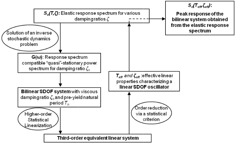
this goal. This point is further clarified in Fig. 1 which presents a flowchart of the proposed

spectrum in Sectio methods linearizat is utilized second-o novel sta issues of oscillator damped bilinear h by the applicabi remarks. m compatible

on 2 based o

for the purp

tion to obtai

d as detailed

order linear S

atistical crite

f using the

r to estimate

response sp

hysteretic SD

European a

ility of the

e power spec

on the work

pose exist in

in a third ord

d in Section

SDOF system

erion for th

e effective

e the peak no

pectra. Furth

DOF system

aseismic co

proposed a

Fig.

ctrum (an eff

k of Vanmar

n the literatur

der linear sy

3), and c) T

m correspon

his task). Fu

linear prope

onlinear resp

her, section

ms exposed to

ode provisio

approach. F

1 Flowchart

ficient metho

rcke [19] an

re (e.g. [21,2

ystem (a form

The reduction

nding to a lin

urthermore,

erties chara

ponse of bili

6 provides n

o the elastic

ons [2] to

inally, secti

t of the prop

od to accomp

nd Cacciola

22]), b) The

mulation due

n of the third

near oscillato

section 5 di

acterizing th

inear hystere

numerical d

c uniform ha

demonstrate

ion 7 includ

posed approa

plish this tas

et al. [20],

e application

e to Asano a

d-order linea

or (section 4

iscusses cer

he derived

etic systems

data pertainin

azard spectru

e the effec

des pertinen

ach.

sk is reviewe

though othe

n of statistic

and Iwan [14

ar system to

4 introduces

rtain practic

linear SDO

from heavil

ng to variou

2. Derivation of response spectrum compatible finite duration stationary stochastic

processes

Field recorded acceleration traces of strong ground motions associated with historic

seismic events exhibit a time-decaying intensity after the initial period of growth. In many

cases a well-defined time window of constant fully-developed intensity is observed in

between the initial build-up and the final decaying parts of these time-histories. This

observation has led several researchers to consider the representation of seismic action by

means of a “quasi-stationary” zero-mean Gaussian acceleration stochastic process g(t) of

finite duration Τs corresponding to the width of the aforementioned window (see e.g.

[19,22-24]). This process is conveniently represented in the domain of frequencies ω by a one-sided

power spectrum G(ω). In relating G(ω) to a response spectrum the response statistics of a

linear single-degree-of-freedom (SDOF) system with natural frequency ωj and ratio of critical

damping ζ base-excited by the process g(t) need to be considered. These statistics can be

expressed in terms of the spectral response moments of order m of the SDOF system given by

the equation (e.g. [25])

( )

( ) (

)

, , , ,

0

,

m

s j m G j m G s

T G H T d

λ =λ =∞

_∫

In the above equation, H(ω,Τs) is the time-dependent transfer function of the considered

system evaluated at a time equal to the duration of g(t). For the purposes of this study, the

following mathematically convenient approximate formula is adopted for the squared

modulus of this transfer function [19]

(

)

(

)

(

)

2

2 2

2 2

1 ,

2

s

j j j

H

ω

ω ω

ζ ω ω

− + , (2)

where

(

)

1 exp 2

j

j sT

ζ ζ

ζω

=

The latter quantity is a fictitious duration-dependent ratio of critical damping to account for

the fact that the response statistics of relatively lightly damped flexible SDOF oscillators may

not reach their stationary (steady-state) values if the duration Ts is not long enough

[19,22-27]. Note that for ζj = ζ Eq. (2) coincides with the squared modulus of the well-known

stationary transfer function of linear SDOF systems. In this case, Eq. (1) provides the

response statistics of SDOF oscillators as if g(t) were a stationary process of infinite duration.

In Fig. 2 the ratio ζj/ζ is plotted versus the natural period of oscillation T= 2π/ωj for several

damping ratios ζ and durations Ts to quantify numerically when the “corrective” damping ζj

of Eq.(3) becomes important in the evaluation of the response statistics of linear SDOF

systems.

Fig. 2 Influence of duration Ts, damping ζ, and natural period T= 2π/ωj on the ratio ζj/ζ.

Let Sα(T,ζ) denote an elastic response pseudo-acceleration seismic spectrum. The

concept of a “peak factor” ηj can be used to establish a relation between Sα and the power

spectrum G(ω) by relying on the equation [19]

2 ,0,

2 _{, .}

a j j j G j

S

π ζ η ω λ

ω

⎛ ⎞

=

⎜ ⎟

⎜ ⎟

⎝ ⎠ (4)

In this regard, ηj can be defined as the ratio of the peak over the standard deviation σ=

The exact determination of the peak factor requires a closed-form solution of the first passage

problem of stochastically excited systems, namely what is the time instant for the response of

the considered oscillator to reach/cross a specific level of intensity with probability p; no such

solution is available in the literature. However, several researchers have proposed various

semi-empirical expressions to obtain reliable estimates of the peak factor for various input

stochastic processes (e.g. [19,24,28,29]). In determining the peak factor ηj appearing in Eq.

(4) the following approximate semi-empirical expression is adopted herein [19]

( )

(

)

{

}

2ln 2 1 exp ln 2

j vj qj vj

η = ⎡_⎢ − − π ⎤_⎥

⎣ ⎦ , (5)

where

(

)

v

λ

π λ

−

= − , (6)

and

2 ,1,

,0, ,2,

1 j G

j

j G j G

q λ

λ λ

= − . (7)

Furthermore, the symbol *

s

T in Eq. (6) denotes a reduced “equivalent stationary response”

duration which takes into account the transient nature of g(t) [19]. It is given by the following

expression

( )

(

)

*

,0,

exp 2 1

/ 2

s j G s s

s j G

T T T T λ λ ⎛ ⎛ ⎞⎞ ⎜ ⎜ ⎟⎟ = − _⎜ − _⎟ ⎜ _{⎝ ⎠}⎟

⎝ ⎠. (8)

The ratio *_/

s s

T T depends on the duration Ts and on the properties of the considered SDOF

oscillator in a similar manner as the ratio ζj/ζ . Specifically, as the product ζωjΤs increases the

ratio of the transient response variances included in Eq. (8) will tend to unity and thus

*

s s

T →T . Note in passing that other approaches to estimate the peak factor for non-stationary

excitations have also been proposed in the literature (e.g. [28,29]). The herein approach due

to Vanmarcke [19] has been adopted due to its relative simplicity which serves well the

By setting p= 0.5 in Eq. (6) the rhs of Eq. (4) estimates the level of the peak

pseudo-acceleration response of a SDOF oscillator excited by the process g(t) not to be exceeded

with probability 50%. Therefore, Sa becomes the median pseudo-acceleration response

spectrum satisfying the following criterion: considering an ensemble of realizations of the

process g(t), half of the population of their response spectra will lie below Sa [19]. Given a

(target) response spectrum Sa, a non-parametric estimate of the power spectrum G(ω)

conforming with the aforementioned criterion can be recursively evaluated at a specific set of

N equally spaced natural frequencies ωk= ω0+ (k-0.5)Δω; k= 1,2,…,N. This is achieved by

using the equation [11,20]

[ ]

(

)

[ ]

2 / ,

4

; 4

0 ; 0

k k

k

i k N

i

k k k k k

k

S

G G

α π ω ζ

ζ _{ω ω ω ω ω}

ω ω π ζ ω η

ω ω

−

= −

⎧ ⎛ ⎞

− Δ < ≤

⎪ ⎜ ⎟

=_⎨ − _{⎝ ⎠}

⎪ _{≤ ≤}

⎩

∑

In the last equation, ωΝ is a “cut-off” frequency above which G(ω) attains negligible values.

Furthermore, ω0 is the lowest value of natural frequency for which Eq. (5) is defined, namely

[11]

( )

(

)

{

}

{

}

0 min ln 2 1 exp ln 2 0

k k k k

v q v

ω

ω = ⎡_⎢ − − π ⎤_⎥ ≥

⎣ ⎦ . (10)

In implementing the recursive numerical scheme defined by Eq. (9) a stochastic process

different than the (unknown) G(ω) needs to be assumed to evaluate the peak factors ηk. For

this task, a viable candidate is a stationary white noise. Under this assumption, the peak

factors ηk appearing in Eq. (9) can be determined by substituting in Eq.(5) [24]

( )

s

k k

T

v

ω

π

= − , (11)

and

2 1

2 ₂

1 2

1 1 tan

1 ₁

k

q ζ

ζ π _ζ

−

⎛ ⎞

⎜ ⎟

= − _⎜ − _⎟

Upon determining the discrete power spectrum G[ω] at ωk frequencies by Eq. (9), the

associated pseudo-acceleration response spectrum D[ωk,ζ] can be approximated using Eqs.

(1)~(8). This task involves the evaluation of the first three response spectral moments which

can be efficiently accomplished by the formulae included in the Appendix A [30]. One can

then compare the thus obtained spectrum D with the target spectrum Sa to assess the error

induced by the various approximations discussed above. In this respect, extensive numerical

experimentation, not included herein for brevity, has shown that for a damping ratio ζ=5%,

which is the most common value adopted in earthquake resistant design applications, and for

durations Ts≥15s, the stationary assumption in the evaluation of the peak factors ηk has a

negligible impact on the effectiveness of Eq. (9) in yielding power spectra compatible with

the target spectrum Sa. However, for lower damping values and/or shorter durations the

transient nature of the assumed white noise process needs to be accounted for. This can be

achieved by substituting in Eq. (12) the duration-dependent damping of Eq. (3) and by using

the reduced duration *

s

T in Eq. (11) given, in the case of white noise, by the expression [19]

(

)

(

)

* _{exp 2} 1 exp 2 ₁

1 exp

k s s s

k s

T T T

T

ζω ζω

⎛ ⎛ − − ⎞⎞

= ⎜_⎜− ⎜_{⎜ − −} − ⎟_⎟⎟_⎟

⎝ ⎠

⎝ ⎠. (13)

. The estimate of G obtained by Eqs. (9-12) using the white noise approximation may

then be modified iteratively to improve the point-wise matching of the response spectrum

D[2π/ωk,ζ] with the target spectrum by means of the following equation written at the Μ-th

iteration [11, 22]

( )

_{[ ]}

_{[ ]}

[

]

( )

_[

_]

2

1 2 / ,

2 / ,

M M a k

k k M

k

S

G G

D

π ω ζ

ω

ω

π ω ζ

+ ₌ ⎛_⎜ ⎞_⎟

⎜ ⎟

⎝ ⎠ . (14)

In this manner, excellent accuracy between D and Sa is achieved within three to four

As a final note of practical interest it is pointed out that the value of the assumed

duration Ts will in general influence the response spectrum compatible power spectrum G(ω)

as obtained from Eqs. (9) and (14). In dealing with response spectra corresponding to a

specific field recorded accelerogram, Ts has the physical meaning of the time window

corresponding to the “stationary” strong part of the ground motion as noted in the beginning

of this section. In such cases, the choice of Ts requires careful consideration to represent

realistically the underlying strong ground motion [22]. However, in this work the target

response spectrum Sa is a “design” Uniform Hazard Spectrum (UHS) which does not

correspond to any physical accelerogram. In this context, the process g(t) defined by its

frequency domain representation G(ω) can be construed as a mathematical tool to represent

the UHS spectrum in a convenient manner that allows for the application of statistical

linearization as detailed in the following sections. Therefore, it is recommended to adopt a

sufficiently large value for Ts depending on the considered damping ratio ζ to facilitate the

numerical work involved in determining effective linear properties according to the proposed

approach outlined in Fig. 1. To this aim, the data presented in Fig. 2 can serve as a guide for

choosing appropriately the duration Ts; this point will be further elucidated in subsequent

sections.

The next step of the herein proposed methodology is to utilize the design spectrum

compatible power spectrum G[ωk] obtained from Eqs. (9) or (14) in conjunction with the

method of statistical linearization. This will lead to the determination of a third-order linear

system associated with a specific bilinear hysteretic oscillator. The mathematical details of

3. Frequency-domain statistical linearization solution for bilinear hysteretic

systems

The inelastic behavior of yielding structures subject to strong ground motions is

commonly modeled in various earthquake resistant design approaches by means of bilinear

hysteretic viscously damped SDOF systems (e.g. [3,31]). The dynamic behavior of such a

system is fully characterized by the following five properties: mass m, viscous damping

coefficient c, pre-yield stiffness k, rigidity α (ratio of the post-yield over the pre-yield

stiffness), and yielding deformation xy. Shown in Fig. 3(a) is a mechanical representation of

the considered system base excited by the acceleration process g(t) [14]. It consists of two

springs, a dashpot, and a Coulomb friction element which slips when the exerted force

becomes greater than (1-α)kxy. A graph of the restoring force of the depicted system for zero

damping is shown in Fig. 3(b) along with the definitions of certain response quantities of

practical interest in the aseismic structural design (i.e. the strength reduction factor R and the

ductility ratio μ). The motion of the bilinear hysteretic system of Fig. 3(a) is governed by the

following system of differential equations with zero initial conditions [14,16]

( )

( )

( )

(

)

(

( ) ( )

)

( )

1

2 _{n n n} 1 , , _y

x t +

ζω

ω

ω

, (15)

( )

( )

(

( ) ( )

)

z t =x t f x t z t x , (16)

where

( ) ( )

(

)

( )

(

( ) ( )

)

( )

{

}

{ }

( )

{

( )

}

{

( )

}

(

)

1 , , 2 , ,

y y

y y y

f x t z t x z t f x t z t x

x U z t x U x t U z t x U x t

=

+ − − − − −

. (17)

and

( ) ( )

(

)

(

{

( )

}

{ }

( )

{

( )

}

{

( )

}

)

2 , , y 1 y y

In the above equations ωn is the pre-yielding natural frequency of the considered

system, x is its response displacement process relative to the motion of the ground

(deformation), and z is an additional “state” corresponding to the relative displacement of the

Coulomb friction element as indicated in Fig. 3 [14]. Further, in the previous equations and

hereafter, the dot over a symbol denotes differentiation with respect to time, and U{·} is the

Heaviside step function, that is, U{v}=1 for v≥0, and U{v}=0 for v<0.

Fig. 3 (a) Mechanical representation of a bilinear hysteretic SDOF system (b) Bilinear

Restoring force-deformation and definitions of the strength reduction factor R and ductility μ.

It is noted that the expression in Eq. (17) ensures that z is bounded within the [-xy, xy]

interval and thus the restoring force from the Coulomb element lies within ±(1-a)kxy [14,16].

Furthermore, the consideration of the z state renders it possible to mathematically express the

bilinear perfectly elasto-plastic hysteretic behavior, corresponding to α=0, via the first order

differential equation Eq. (16) [32]. The latter equation reflects that the rate of change of z is

equal to x (no slip occurs) for |z|<xy and becomes zero for |z|=xy. More importantly, the

consideration of the z state allows for the employment of a statistical linearization scheme

proposed to treat stochastically excited non-linear multi-degree-of-freedom structural systems

scheme to the system of the non-linear Eqs. (15) and (16) yields the system of linear

differential equation [14]

( )

( )

( )

(

)

(

( )

( )

)

( )

1 2

2 n n n 1

x t +

ζω

ω

ω

(19)

and

( )

( )

( )

z t +C x t +C z t = . (20)

The four equivalent linear coefficients C1to C4 appearing in the last two equations are

determined by requiring minimization of the mean square error in replacing Eqs. (15) and

(16) by Eqs. (19) and (20), respectively [12]. Implementing the procedure delineated in [12]

the following expressions for the aforementioned coefficients are derived

( ) ( )

(

)

( )

(

)

₍

₎

2 2 _{2 2}

, ,

1

exp

2 1 2 1 2 1

y

y y y

z

x z _{x z z}

f x t z t x C E

x t

x x x

erfc

σ ρ

πσ σ ρ πσ σ ρ σ ρ

⎧∂ ⎫ ⎪ ⎪ = _{⎨ ⎬}= ∂ ⎪ ⎪ ⎩ ⎭ ⎛ ⎞ ⎛ ₋ ⎞ − _{⎜ ⎟ ⎜ ⎟} − _{⎜ ⎟}+ _{⎜ ⎟} − − ⎜ − ⎟ ⎝ ⎠ _{⎝ ⎠} , (21)

( ) ( )

(

)

( )

( )

2 2 y 1

z

y

y

x z

f x t z t x C E

z t

x v

erf v erf dv

σ

ρ

σ π ρ

∞ ⎧∂ ⎫ ⎪ ⎪ = _{⎨ ⎬}= ∂ ⎪ ⎪ ⎩ ⎭ ⎛ ⎞ ⎡ ⎛ ⎞⎤ ⎜ ⎟ + − − ⎢ ⎜_⎜ ⎟_⎟⎥ _{⎜ ⎟} − ⎢ ⎝ ⎠⎥ ⎣ ⎦

∫

( )

(

( ) ( )

)

( )

, , y

x t f x t z t x

C E C

x t ⎧∂⎡ ⎤⎫ ⎪ _{⎣ ⎦}⎪ = − _{⎨ ⎬}= − ∂ ⎪ ⎪ ⎩ ⎭ , (23) and

( )

(

( ) ( )

)

( )

(

)

(

)

2 2 2

2 2 2

2 ₂

, ,

1

exp 1 exp

2 2 1

2 _{2 1}

y

y x y y x y

z z z

z _z

x t f x t z t x

C E

z t

x x x x

erf

ρ σ ρ σ ρ

σ πσ ρ σ

σ π _{σ ρ}

( )

{ }

{ }

( )

{

( ) ( )

}

2 _; 2 _;

x z

z x

E x t z t E x t E z t

σ

σ

ρ

σ σ

In the previous equations and henceforth E{} denotes the mathematical expectation operator.

Moreover, erf() and erfc() are the standard error and complementary error functions defined

by the expressions

( )

( )

( )

( )

0

2 u_{exp ; 1}

erf u w dw erfc u erf u

π

=

∫

From the Eqs. (21) to (25) it is seen that the equivalent linear coefficients C1 to C4 to

be determined depend on the variance of the processesxand z, that is 2

x

σ and σz2 , and on

their cross-varianceE xz

{ }

the spectral input/output relations for linear systems is used to calculate these response

moments [35]. This formulation is significantly different from the state-space approach

commonly considered in the literature for the purpose [14,16]. It facilitates the numerical

implementation of the herein considered approach in which the input spectrum G(ω) is given

in a non-parametric form known at discrete frequencies as explained in the previous section.

Specifically, the system of Eqs. (19) and (20) is first written in matrix form as

( )

( )

( )

( )

( )

( )

( )

x t x t x t g t

z t z t z t

⎧ ⎫ ⎧ ⎫ ⎧ ⎫ ⎧− ⎫ ⎪ ⎪₊ ⎪ ⎪₊ ⎪ ⎪ ⎪₌ ⎪ ⎨ ⎬ ⎨ ⎬ ⎨ ⎬ ⎨ ⎬ ⎪ ⎪ ⎪ ⎪ ⎪ ⎪ ⎪ ⎪ ⎩ ⎭ ⎩ ⎭ ⎩ ⎭ ⎩ ⎭

M C K

, (27)

where

(

)

(

)

1 2

3 4

1 0 2 1 0 1

; ;

0 0 1 0

n a nC a n a nC

C C

ζω

ω

ω

ω

⎡ + − ⎤ ⎡ − ⎤

⎡ ⎤

=_{⎢ ⎥} =_{⎢ ⎥} =_{⎢ ⎥}

⎣ ⎦ ⎣ ⎦ ⎣ ⎦

M C K . (28)

Next, the response power spectrum matrix of the system of Eqs. (27) is expressed as

( )

( )

_{( )}

_{( )}

( )

( ) ( )

( )

0 0

xx xz zx zz

B B G

B B

ω

ω

ω

ω

ω

ω

ω

ω

B H H , (29)

( )

( )

_{( )}

( )

_{( )}

(

)

ω

ω

ω

ω

ω

ω

ω

−

⎡ ⎤

=_{⎢ ⎥}= − + +

⎣ ⎦

H M C K , (30)

and the superscripts (*) and (-1) stand for complex matrix transposition and matrix inversion,

respectively. Then, the required response variances are determined from the elements of the

matrix B using the equations [35]

( )

( )

( )

( )

[ ]

2 2

2 2 2 4 2 4

3 3 0 0 0 0 0 N k

x xx k k

j _k j

j k j

j j

i C i C

B d G d G

i A i A

ω

ω

σ

ω

ω ω

ω

ω ω

ω ω

ω

ω

ω

=

_∫

_∫

∑

∑

∑

( )

( )

( )

( )

[ ]

2 3 3

3 3

0

0 0

0 0

N

z zz k

j _k j

j k j

j j

i C i C

B d G d G

i A i A

ω

ω

σ

ω ω

ω ω

ω

ω

ω

ω

∞ ∞

=

= =

− −

=

_∫

_∫

∑

∑

∑

in which i= −1_,and

(

)

(

)

(

)

(

)

2 2 2 2

0 4 1 1 4 2 3

2

2 4 1 3

; 2 1 1 ;

2 1 ; 1

n n n n n

n n

A a C A a a C C a C C

A C a C A

ω ω ζω ω ω

ζω ω

= = + + − − −

= + + − = . (33)

Finally, the cross-variance term appearing in Eqs. (21) to (25) is determined by the equation

{ }

3 z C E xz C σ = − . (34)

The latter equation is derived by multiplying Eq. (20) by z(t), taking the mathematical

expectation and noting that E z t z t

{

( ) ( )

}

integrals appearing in the calculation of the response variances in Eqs. (31) and (32) can be

approximated by a finite summation. This can be done by using the frequency domain

discretization scheme introduced in the numerical evaluation of the input spectrum G(ω) at a

discretization step Δω and can be readily improved, at will, by straightforward interpolation

schemes.

To this end, Eqs. (21)~(24), (31), (32), and (34) form a system of seven non-linear

equations with seven unknowns, namely, C1~C4, σ_x2,σz2, and E xz

{ }

readily written as a standard minimization problem and solved numerically by any

appropriate optimization routine starting from a reasonable initial guess. In all of the ensuing

numerical work a built-in optimization algorithm of MATLAB® using a trust region dog-leg

search method is used to solve the aforementioned system of equations [36]. Furthermore,

standard MATLAB® built-in routines are used for the numerical evaluation of the error and

complementary error functions (Eq. (26)), and of the integral appearing in Eq. (22).

Alternatively, the latter integral can be evaluated at each iteration required by the

optimization algorithm using the series expansion reported in [14].

Upon determination of the C1 to C4 coefficients, an “equivalent” linear third-order

system (ELS) involving the x, x, and z states is established governed by the differential Eqs. (19) and (20). Note that it has been established in the literature [12,14-16], both theoretically

and through numerical experimentation, that this ELS captures the response statistics of

bilinear hysteretic systems exhibiting strong nonlinear behavior more accurately than a

second-order ELS derived by the statistical linearization approach due to Caughey [12,13].

However, this third order ELS cannot be readily related to a response/design spectrum

pertaining to the peak response of linear SDOF oscillators. To this end, in the next section a

novel approach to reduce the system order is introduced by relying on a specific statistical

4. Derivation of effective linear properties from the 3rd order equivalent linear

system

Let y be the normalized by xy deformation of an “auxiliary” linear SDOF oscillator of

critical viscous damping ζeff and natural frequency ωeff base excited by the acceleration

process g(t). The governing equation of motion of this auxiliary system reads as

( )

( )

( )

( )

2 eff eff eff / y

y t +

ζ ω

ω

, (35)

and zero initial conditions apply. For the purposes of this work, it is desired to relate the

above second order linear system to the third order ELS of Eqs. (19) and (20). This can be

accomplished by enforcing equality of the stationary variances of the processes x(t) and y(t).

That is,

( )

{ }

₍

₎

( )

₍

₎

2 2 2 ,0, 2 2 2 2 0 / / 2 y

x eff G y

eff eff eff

G x

E x t

ω

σ

ω λ

ω ω

ζ ω ω

∞

= = =

− +

∫

and of the stationary variances of the processes x t

( )

( )

( )

(

)

(

)

x eff G y

eff eff eff

G x

d x

ω

ω

σ

ω λ

ω ω

ζ ω ω

∞

= =

− +

∫

. (37)

The variance appearing in the lhs of Eq. (36) can be calculated by the expression

( )

( )

( )

[ ]

2 2

2 4 4

3 3 0 0 0 0 N k x k

j _k j

j k j

j j

i C i C

G d G

i A i A

ω

ω

σ

ω ω

ω

ω

ω

ω

=

_∫

∑

∑

∑

At this stage, the coefficients C1 to C4 are known from solving the nonlinear system of

equations considered in the statistical linearization solution of the previous section. Thus, 2

x

σ

is readily calculated numerically in the same manner as the variances in Eqs. (31) and (32).

The variance appearing in the lhs of Eq. (37) is also a known quantity from the solution of the

nonlinear equations which can be solved for the two unknown effective linear properties ζeff

and ωeff corresponding to the considered auxiliary linear SDOF oscillator. To this aim, the

same optimization algorithm used to obtain the statistical linearization solution can be

employed. At each iteration of the optimization algorithm, the expressions included in the

Appendix A are used to numerically evaluate the integrals in Eqs. (36) and (37) in a

computationally efficient manner.

Note that in computing the response variances appearing in Eqs. (36)~(38) the fact

that the duration Ts of the stationary process g(t) is finite has not been explicitly taken into

account. However, as already suggested in section 2, it is possible to consider a long enough

duration Ts in deriving the response spectrum compatible power spectrum G(ω) so that the

effective pair of properties Teff= 2π/ωeff and ζeff correspond to a point on the plots of Fig. 2 for

which the corrective damping defined in Eq. (3) coincides with the value of ζeff. That is,

exp(-2 ζeff ωeff Ts)≈0. Under this condition, it can be argued that the transient nature of the input

process g(t) does not need to be taken into account and one can treat the response statistics of

the linear systems defined by Eqs. (19) and (20), and by Eq. (35) as being stationary.

Additional comments on this issue are provided in a following section in light of numerical

data corresponding to a large range of bilinear hysteretic systems.

5. Peak nonlinear response estimation using the effective linear properties

The preceding three sections provided the theoretical background to derive effective

linear properties (ELPs) (ζeff and ωeff) for viscously damped bilinear hysteretic systems

exposed to a given code-prescribed elastic response pseudo-acceleration spectrum Sα(Τ,ζ)

following the proposed approach outlined in Fig. 1. The salient advantage of this approach is

that these ELPs depend not only on the properties of the nonlinear systems considered,

ratio α, but also to the specified response spectrum Sα(Τ,ζ) [10,11]. In this regard, it can be

argued that a reasonable estimate of the peak deformation of bilinear hysteretic oscillators

can be determined by the expression

( )

{ }

(

) (

) (

)

, , 5%

max_t a eff eff eff, eff a eff

eff eff

S T S T

x t

ζ

ζ

ζ

ω

ω

=

≈ = . (39)

That is, by using a family of response spectra corresponding to various damping ratios. Such

response spectra are commonly defined in most of the earthquake resistant design

applications by means of multiplying a “reference” design spectrum corresponding to ζ=5%

by a reduction factor B. In general, it is known that this factor depends on the damping ratio

and on the natural period of oscillation, and, thus, on the ELPs as suggested in the last

equation (see e.g. [9,37]). In this manner, the need for numerically integrating the non-linear

Eqs. (15) and (16) of motion for an ensemble of seismic accelerograms compatible with the

considered response/design spectrum is by-passed.

Obviously, the reliability of the estimated peak value will depend on the severity of the

nonlinear response induced by the seismic action. Further, it will reflect the well-quantified

approximations associated with the statistical linearization method [12,15]. Also, it will

depend on the effectiveness of the adopted B factor to predict the peak response of linear

SDOF oscillators for different ratios of critical damping which remains an issue of open

research [9,37]. To this end, it is noted that in case dependable response spectra are not

available for damping ratios other than ζ, an estimate of the peak non-linear response can be

achieved by the equation

( )

{

}

max eff x

t x t ≈η σ , (40)

which relies on the concept of the peak factor and the fact that the variance of x(t) has been

Eqs. (1)~(8) by setting p=0.5, ζ=ζeff, and ωj=ωeff and by considering the power spectrum G(ω)

and the duration Tsused to obtain the ζeff and ωeff pair of ELPs.

6. Numerical application to the EC8 design spectrum

6.1 EC8 compatible effective linear properties of bilinear hysteretic systems

The elastic response (uniform hazard) spectrum of the current aseismic code provisions

effective in Europe (EC8) [2] is considered herein as a paradigm of assessing the usefulness

and applicability of the proposed approach. Specifically, the EC8 (target) pseudo-acceleration

response spectrum for peak ground acceleration 0.36g (g= 981cm/sec2), ground type “B” and

damping ratio ζ= 5% (gray thick line in Fig. 4(a)), is considered to represent the induced

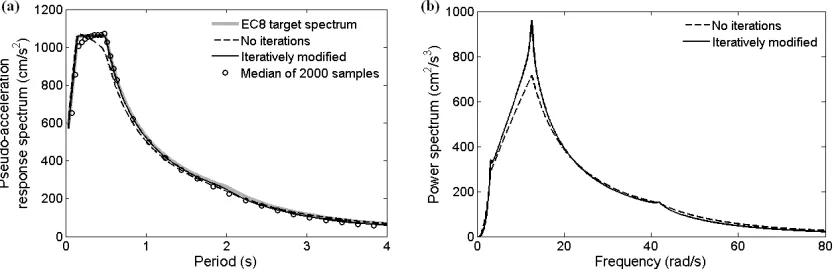
seismic action. The broken line of Fig. 4(b) corresponds to a discrete power spectrum

compatible with the considered EC8 target spectrum computed by means of Eq. (9) assuming

Ts= 20s, Δω= 0.1rad/s, and using Eqs. (11) and (12) to estimate the peak factors ηk. Further,

this initial power spectrum is modified by performing four iterations using Eq. (14). The

obtained modified spectrum is also shown in Fig. 4(b). The pseudo-acceleration response

spectra associated with the two power spectra of Fig. 4(b) are plotted in Fig. 4(a) and

compared with the target spectrum. These response spectra have been calculated analytically

using Eqs. (1)~(8). It can be seen that the response spectrum corresponding to the initial

power spectrum cannot trace closely the target spectrum near the “corner period” of 0.5s

which signifies the end of the flat segment of constant spectral ordinates. However, the

iteratively matched power spectrum characterized by a quite prominent spike at a frequency

of 2π/0.5= 12.6 rad/s yields a significantly better matching with the target spectrum along the

whole axis of natural periods. This is further confirmed by considering the median spectral

ordinates of an ensemble of 2000 20s long stationary signals compatible with the iteratively

random field simulation technique based on an auto-regressive-moving-average filter [38].

The latter Monte Carlo-based simulation analysis ensures numerically that the criterion

prescribed by Eq. (4) for p=0.5 is satisfied by the iteratively modified spectrum considered.

Fig. 4 (a) Target EC8 spectrum, response spectra corresponding to the power spectra shown in panel (b) and median response spectrum from 2000 simulated signals. (b) Power

spectra compatible with the EC8 spectrum of panel (a).

Next, the iteratively modified power spectrum of Fig. 4(b) is used to obtain effective

linear properties (ELPs) Teff= 2π/ωeff and ζeff via the statistical linearization-based method

detailed in sections 3 and 4 for various bilinear hysteretic oscillators. In particular, the

seven-by-seven system of nonlinear Eqs. (21)~(24), (31), (32), and (34) is solved in series with the

two-by-two system of nonlinear Eqs. (36) and (37) for viscously damped bilinear oscillators

with ζ=5%, pre-yield natural period Tn=0.5s, 1.0s, 1.5s, and 2s (Tn= 2π/ωn), rigidity ratios α

ranging from 0.5 to 0.05 and for several values of yielding deformation xy. The latter is

treated as the “free” parameter to represent different levels of nonlinear behavior. The thus

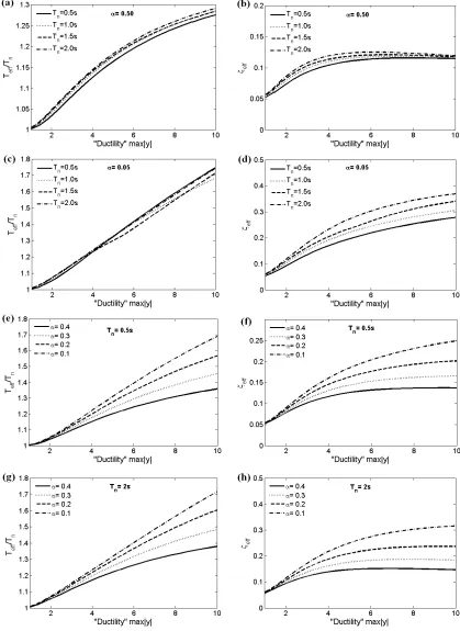
obtained ELPs are plotted in Fig. 5 against the “ductility” max|y| defined in Eq. (35) which

quantifies the severity of the nonlinear response. These data serve to provide numerical

evidence that the herein proposed approach yields results that are in reasonable agreement

In general, the departure from the linear response quantified by larger values of max|y|

yields “softer” effective linear systems characterized by longer natural periods. It is noted,

however, that the ratio of Teff/Tn is not quite sensitive to changes in the pre-yield stiffness for

a fixed rigidity α and ductility level (panels (a) and (c) in Fig. 5). This ratio appears to be

more influenced by the rigidity α and increases at a significantly higher rate, as max|y|

increases for bilinear systems closer to the ideal elasto-plastic one, that is, as α→0 (panels (e)

and (g) in Fig. 5). Accordingly, the effective damping ratio increases with max|y| to account

for the increased energy dissipation through more severe plastic/ hysteretic behavior of the

corresponding nonlinear systems. Similar trends for ELPs of bilinear hysteretic oscillators

subject to white noise excitation have been reported in the literature [e.g. 13, 39].

Notably, it is observed that for all bilinear systems considered herein, reflecting a large

range of systems pertinent to earthquake engineering applications, ζeff increases quite rapidly

with ductility and at a much higher rate than Teff. Consequently, in all cases plotted in Fig. 5

the product ωeffζeff tend to increase as stronger nonlinear behaviour is exhibited. It turns out

that the quantity exp(-2ζeff ωeff Ts) for Ts=20s negligible in all cases considered in Fig. 5.

Thus, by referring to Fig. 2, it is suggested that for bilinear systems with ζ=5% viscous

damping and Tn≤2s choosing a duration of at least Ts=20s in deriving the response spectrum

compatible power spectrum G(ω) circumvents the need to consider the transient nature of the

response moments appearing in Eqs. (36)~(38). In this regard, the underlying process g(t) can

be treated as stationary in the context of the proposed approach of Fig. 1. Clearly, if bilinear

systems with smaller than 5% ratio of viscous damping are considered, a longer duration may

be required to be adopted in treating g(t) as stationary. If for any practical reason this is not

possible, then the transient nature of the response moments in Eqs. (36)~(38) can be

increased fictitious damping ratio dependent on the duration and the natural frequency of the

considered linear systems [19,22,23].

Note that in obtaining the plots in Fig. 1, the ductility max|y| has been estimated for

each pair of effective linear properties by using the considered EC8 elastic spectrum without

6.2 Estimation of peak nonlinear response using the effective linear properties

In the preceding sub-section ELPs (ζeff and ωeff) have been derived for several viscously

damped bilinear hysteretic systems exposed to the EC8 response spectrum of Fig. 4(a)

following the proposed approach outlined in Fig. 1. From the discussion included in section 5

it is clear that these ELPs can be used in conjunction with the EC8 spectrum to estimate the

peak nonlinear response of the considered systems. This is done by substituting in Eq. (39)

the B factor for T=Teffand ζ=ζeff prescribed by EC8 which for ground type “B” reads as [2]

(

)

8

10

1 2.5 1

0.15 5

; 0 0.15

, _{1 10}

10

; 0.15 4

5

EC

T

T

B T _T

T

ζ ζ

ζ

⎧ ⎛ ⎞

+ −

⎪ ⎜ ₊ ⎟

⎪ ⎝ ⎠ _{≤ ≤}

⎪

=_{⎨ +}

⎪

⎪ _{≤ ≤}

⎪ +

⎩

, (41)

where ζ needs to be expressed as a percentage (i.e. ζ→5 for ζ=5%). The aforementioned

nonlinear peak response estimation step can perhaps be better understood graphically as

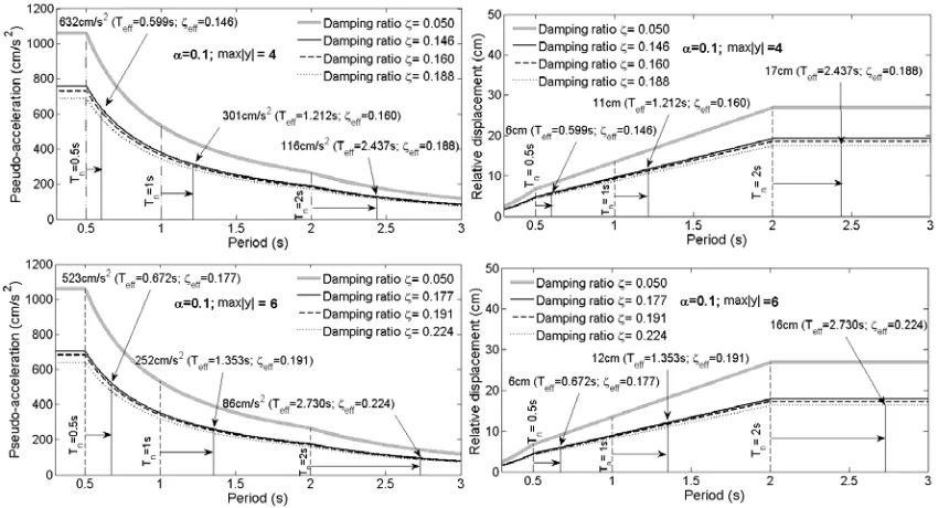
shown in Fig. 6 in terms of deformations (panels (b) and (d)) and in terms of

psedo-acceleration (panels (a) and (c)) for various bilinear hysteretic systems. In particular, consider

a specific viscously damped bilinear hysteretic oscillator with damping ratio ζ= 5% and

pre-yield natural period Tn exposed to theEC8 elastic response spectrum (vertical broken lines).

One can move, following the horizontal arrows, to a vertical solid line corresponding to an

effective linear system characterized by Τeff and ζeff obtained by the statistical linearization

based methodology herein adopted and “read” the related spectral ordinate. In this manner, an

estimate of the peak response of the considered structural system is achieved without the need

to have available suites of spectrum compatible accelerograms and to numerically integrate

Fig. 6 Peak response estimation using the effective linear properties in conjunction with the EC8 elastic spectrum for various values of damping.

As a final note, it is pointed out that the “ductility” in the plots of Fig. 5 and Fig. 6 has

been computed by

( )

{

}

(

) (

)

, 5%

max _{EC eff}, _eff a eff .

y eff

S T y t B T

x

ζ

ζ

ω

= (42)

6.3 Assessment of peak nonlinear response predictions via Monte Carlo simulation

In this section the potential of the EC8 compatible ELPs plotted in Fig. 5 to provide

reasonable estimates of the peak response of the corresponding bilinear hysteretic systems is

assessed in a Monte Carlo simulation context. To this aim, an ensemble of 250 artificial

non-stationary accelerograms compatible with the EC8 spectrum of Fig. 4(a) are considered.

These signals have been generated by a wavelet-based stochastic approach recently proposed

by Giaralis and Spanos [40]. The time-history of an arbitrarily chosen accelerogram is plotted

in Fig. 7 along with its velocity and displacement trace. Furthermore, pertinent statistics of

pseudo-acceleration are included on the same figure and compared with the target EC8 spectrum. In

particular, the average response spectrum of the 250 considered accelerograms practically

coincides with the EC8 spectrum. Thus, these signals are consistent with the compatibility

criterion utilized in deriving the input power spectrum G(ω) (see also Fig. 4) considered in

obtaining the ELPs of Fig. 5.

Fig. 7 Response spectra statistics and time-history traces of a sample of 250 non-stationary artificial accelerograms compatible with the EC8 spectrum of Fig. 4(a).

Next, the aforementioned accelerograms are used to excite various bilinear hysteretic

systems. The nonlinear response is obtained by numerical integration of the nonlinear Eqs.

(15) and (16). The standard constant acceleration Newmark’s scheme, incorporating an

iterative Newton-Raphson algorithm to treat locally the discontinuities of the piecewise linear

force-deformation law, is used for the task [3]. In Fig. 8 the ductility of certain bilinear

systems (dots of various shapes) computed from ensemble averaging of the systems’

nonlinear responses is plotted versus the strength reduction factor R (R-μ-Tn relationships); R

is defined in Fig. 3(b) as the ratio of the peak demand in terms of elastic restoring force fel for

a particular excitation over the yielding strength fy of the bilinear oscillator. In the same tigure

the, thus, obtained R-μ-Tn relationships are examined vis-à-vis the peak response normalized

whose properties (ELPs) have been derived as detailed in the previous sub-section from the

considered nonlinear systems.

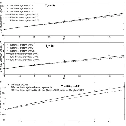
In general, the quality of the achieved approximation of the peak nonlinear responses

by the peak responses of the corresponding heavily damped linear oscillators deteriorates as

the level of nonlinear behavior increases. That is, for smaller rigidity ratios α and for larger

strength reduction factors R. This is expected and reflects the approximations involved in the

statistical linearization step discussed in section 3 (see also [12,13]).

Overall, satisfactory matching of the average peak values for the considered ensemble

of accelerograms is achieved for bilinear hysteretic systems of rigidity ratios as small as

α=0.1~0.2 and for a wide range of strength reduction factors (Fig. 8 (a) and (b)). Further, Fig.

8(c) provides a comparison of the accuracy achieved between the herein proposed approach

and the earlier one of Giaralis and Spanos [11] which utilizes a second-order statistical

linearization scheme based on the work of Caughey [13]. The latter is computationally less

involved, requiring the solution of only one three-by-three system of nonlinear equations.

However, the herein proposed approach yields significantly better results for bilinear systems

Fig. 8 Mean peak responses of various bilinear hysteretic and of their corresponding effective linear systems subject to the 250 EC8 compatible accelerograms considered in Fig. 7.

7. Concluding Remarks

A novel statistical linearization based approach has been proposed for deriving

effective linear properties (damping ratio and natural frequency) (ELPs) corresponding to

linear SDOF oscillators for viscously damped bilinear SDOF hysteretic systems subject to

seismic excitation defined by a response/design spectrum. These ELPs are determined by

solving one seven-by-seven system and one two-by-two system of non-linear equations. The

replaces the bilinear system by a third order linear system. The second system of equations is

associated with a system reduction step to capture certain of the response statistics of the

third order linear system by a second order SDOF oscillator response statistics. Both

solutions involve the employment of a numerically derived power spectrum representing in

the frequency domain a “quasi-stationary” process of finite duration satisfying a certain

probabilistic compatibility criterion with the given response spectrum. This criterion

conforms with common aseismic code provisions for acceleration time-histories. That is, the

average response spectrum of samples belonging to the considered process is close to the

given response (uniform hazard) spectrum. An efficient recursive formula has been used to

determine the required power spectrum satisfying the aforementioned compatibility criterion.

A salient feature of the thus obtained ELPs is that they are explicitly associated with both the

pre-specified response spectrum and the considered bilinear system. In this respect, it is

possible to obtain reliable estimates of the peak nonlinear response by utilizing the ELPs in

conjunction with the given elastic response spectrum modified appropriately to account for

different values of damping ratio. In this manner, the peak nonlinear response is obtained

from heavily damped elastic response spectra without integrating the nonlinear equations of

motion. This is done without considering ensembles of response spectrum compatible

scaled/modified field recorded and/or artificially generated accelerograms. The potential of

the ELPs to serve this purpose has been ascertained by pertinent numerical results associated

with the elastic response uniform hazard spectrum prescribed by the aseismic code

regulations effective in Europe (EC8). Specifically, EC8 compatible ELPs corresponding to

various bilinear systems of different rigidity ratios, pre-yield stiffness, and yielding

deformations have been obtained. Further, strength reduction-ductility-natural period (R-μ

-T-n) relationships have been derived for the considered hysteretic systems and for the associated

EC8 compatible non-stationary time-histories obtained via a wavelet-based stochastic

approach. For these time-histories reliable estimates of the nonlinear average peak response

have been obtained for rigidity ratios of the order of 10~20% and for strength reduction

factors of the order of 5. In this regard, it has been demonstrated that the proposed approach

which employs a high-order (third-order) statistical linearization technique and a novel order

reduction step provides significantly better compared to the earlier work of the authors in [11]

estimates of the peak inelastic response of bilinear inelastic/hysteretic oscillators exhibiting

strong nonlinear behavior. Further, the developed approach can potentially be modified to 

accommodate versatile smooth nonlinear systems whose hysteretic component can be represented 

by means of an additional differential equation, such as the Bouc‐Wen model [41]. 

Appendix A.

Consider a power spectrum G corresponding to a quasi-stationary stochastic process

known at a set of discrete equally spaced frequencies ωq , that is G[ωq]= Gq, where ωq= ω0+

(q-0.5)Δω, with q= 1,2,…,M and ω0 is given by Eq (10). Using the “grid” ωp= ω0+ (p-1)Δω;

p= 1,2,…,M+1, to discretize the frequency axis, the first three response spectral moments of

Eqs. (1)~(3) can be numerically evaluated using the formula [30]

, , , ,

1

M

n m G n m p p p

J G

λ

=

=

∑

in which

(

)

(

)

(

)

(

)(

)

(

(

)(

)

)

(

)

(

)

(

(

)(

)

)

, , 2 ₂

1 1 1

2 1

2 2

1 1

2 ₂

1 1 1

3 4 3

2 ₂ 2

1

ln 2

1 sgn tan

2

ln tan

2

p D n m p

p D

p p p p

D

p D p D p D p D

p D _D p p

p D p D p D c x J c c c x x

c c c

c c

x x x

c c

c

ω ω

ω ω

ω ω ω ω

ω π

ω ω ω ω ω ω ω ω

ω ω _ω ω ω

ω ω ω ω

where ₁ 2

D n n

ω

ω

ζ

2 1 0 2 2 1 3 2 2 4 2

1 ₀ 1

4 4

1 1 ₀

2 4 1,

;

1 ₀ 1 0 ,

4 4

1 1 ₀

2 4

n D D

n D

i

n D D

n D

x

r

x i m

r r

x i m

r x

ω ω ω

ω ω

ω ω ω

ω ω ⎡₋ ⎤ ⎢ ⎥ ⎢ ⎥ ⎧ ⎫ ⎢ ⎥ ⎧ ⎫ ⎪ ⎪ ⎢ ⎥ _{⎧ =} ⎪ ⎪_{=⎢ ⎥}⎪ ⎪ ₌ ⎨ ⎬ _{⎢ ⎥}⎨ ⎬ ⎨ _≠ ⎩ ⎪ ⎪ _{⎢ − ⎥ ⎩ ⎭}⎪ ⎪ ⎪ ⎪ ⎩ ⎭ ⎢ ⎥ ⎢ ⎥ − ⎢ ⎥ ⎣ ⎦ . (C) References

[1] McGuire RK. Seismic Hazard and Risk Analysis. Monograph MNO-10. Oakland:

Earthquake Engineering Research Institute; 1995.

[2] CEN. Eurocode 8: Design of Structures for Earthquake Resistance - Part 1: General

Rules, Seismic Actions and Rules for Buildings. EN 1998-1: 2004. Brussels: Comité

Européen de Normalisation; 2004.

[3] Chopra AK. Dynamics of Structures. Theory and Applications to Earthquake

Engineering. 2nd ed. Englewood Cliffs: Prectice-Hall; 2001.

[4] Veletsos AS, Newmark NM. Response spectra for single-degree-of-freedom elastic and

inelastic systems. Rep. No.RTD-TDR-63-3096. Vol. III. Albuquerque: Air Force

Weapons Laboratory; 1964.

[5] Chopra AK, Chintanapakdee C. Inelastic deformation ratios for design and evaluation of

structures: Single-degree-of-freedom bilinear systems. J Struct Eng ASCE 2004;130:

1309-19.

[6] Miranda E, Ruiz-García J. Evaluation of approximate methods to estimate maximum