Comparative performance evaluation of latency and link dynamic power consumption modelling algorithms in wormhole switching networks on chip

(1)

This is a repository copy of Comparative performance evaluation of latency and link dynamic power consumption modelling algorithms in wormhole switching networks on chip.

White Rose Research Online URL for this paper: http://eprints.whiterose.ac.uk/100154/

Version: Accepted Version

Article:

Harbin, James orcid.org/0000-0002-6479-8600 and Soares Indrusiak, Leandro

orcid.org/0000-0002-9938-2920 (2016) Comparative performance evaluation of latency and link dynamic power consumption modelling algorithms in wormhole switching networks on chip. Journal of systems architecture. pp. 33-47. ISSN 1383-7621 https://doi.org/10.1016/j.sysarc.2016.01.002

Reuse

Items deposited in White Rose Research Online are protected by copyright, with all rights reserved unless indicated otherwise. They may be downloaded and/or printed for private study, or other acts as permitted by national copyright laws. The publisher or other rights holders may allow further reproduction and re-use of the full text version. This is indicated by the licence information on the White Rose Research Online record for the item.

Takedown

If you consider content in White Rose Research Online to be in breach of UK law, please notify us by

(2)

Comparative Performance Evaluation of Latency and

Link Dynamic Power Consumption Modelling

Algorithms in Wormhole Switching Networks On Chip

James Harbin1,∗_{, Leandro Soares Indrusiak}1

Real-Time Systems Group, Department of Computer Science, University of York, UK

Abstract

The simulation of interconnect architectures can be a time-consuming part

of the design flow of on-chip multiprocessors. Accurate simulation of

state-of-the art network-on-chip interconnects can take several hours for realistic

application examples, and this process must be repeated for each design

it-eration because the interactions between design choices can greatly affect

the overall throughput and latency performance of the system. This

pa-per presents a series of network-on-chip transaction-level model (TLM)

al-gorithms that provide a highly abstracted view of the process of data

trans-mission in priority preemptive and non-preemptive networks-on-chip, which

permit a major reduction in simulation event count. These simulation

mod-els are tested using two realistic application case studies and with synthetic

traffic. Results presented demonstrate that these lightweight TLM

simula-∗_{Corresponding author: Telephone +44 (0)1904 325550, Fax +44 (0)1904 325599}

Email addresses: [email protected](James Harbin),

(3)

tion models can produce latency figures accurate to within mere flits for the

majority of flows, and more than 93% accurate link dynamic power

con-sumption modelling, while simulating 2.5 to 3 orders of magnitude faster

when compared to a cycle-accurate model of the same interconnect.

Keywords: network on chip, transaction level modelling, TLM, NoC

modelling, simulation models, dynamic power consumption

1. Introduction

As the number of cores upon on-chip multiprocessors and system-on-chip

(SoC) devices has increased, inter-core communication has become a critical

design issue. The design architecture of the NoC (network-on-chip) is a vital

factor in performance tuning, given the large influence it has upon

commu-nication latency and power consumption. As a result of the highly dynamic

nature of application traffic and the potential for interactions between

traf-fic during transmission, most design flows use simulation rather than static

analysis to evaluate the power and latency performance delivered by a

can-didate NoC architecture. NoC interconnect simulation (as distinct from the

full system simulation including execution of code upon processing elements)

has been identified as an important research issue [1]. The design space of

viable NoCs for multicore or SoC problems spans a wide range of candidate

architectures and topologies, and is further expanded by the possible

vari-ability in application task mapping decisions. Particularly during the early

(4)

with as little impact upon accuracy as possible, allowing the design space

to be explored rapidly. Therefore, methodologies other than cycle-accurate

simulation are promising as candidates to rapidly explore the NoC design

space.

This paper specifies and evaluates a family of NoC simulation models

which are both fast and accurate in comparison to cycle-accurate references.

Two NoC architectures are considered which can be accurately described

us-ing transaction-level modellus-ing (TLM). The models assume delay-sensitive

applications that have certain timing constraints, and therefore the

appli-cation model includes priorities used in arbitration decisions. Since these

application models typically require one flow to be prioritised over another,

priority preemptive NoCs following the example of QNoC [2] are the first

architecture assumed. However, given that priority preemptive NoC

archi-tectures have higher silicon area requirements for implementation, a

non-preemptive architecture is also considered and evaluated.

The definition of TLM assumed in this work is that of Cai and Gajski

[3], in which components are either transaction initiators, targets or

inter-connects. The relationship of our models to the TLM definitions specified

by Cai and Gajski is considered in Section 5. Compared to cycle-accurate

models, the proposed TLM algorithms are simplified to reduce the frequency

of simulation events. Events are generated only upon flow admission, flow

removal or when simulation state must be updated to ensure consistency.

(5)

every data flit through arbiters, routers and other simulator-level elements

permits the reduction of simulation event count by orders of magnitude.

A fine-grained cycle-accurate model can offer precise simulation of the

NoC internals, including the occupation and free status of particular buffers.

However, in order to improve execution time performance and reduce

simu-lation algorithm complexity, the buffer occupation of intermediate routers is

not considered within the TLM models described in this paper. Even under

the design structure of a transaction level model, several design choices are

possible regarding the abstraction levels chosen, with resulting implications

for timing performance and accuracy. In our earlier work [4], [5], [6] the entire

route was be treated as a single unified abstraction when making contention

decisions. Although this modelling approach is simple and its execution

tim-ing performance favourable, heavy contention requires a more fine-grained

approach to improve timing accuracy.

The major novelty in this paper is the presentation of the TLM model

TLM-NPD, which provides a finer locking granularity at the level of

individ-ual links and the ability to model flow behaviour in single-cycle increments

in case of contention. The further intent of this paper is to comparatively

as-sess and evaluate the simulation latency accuracy and execution time

perfor-mance of our family of transaction level models TLM-PRE [4], [5], TLM-NP

[6] and TLM-NPD, compared to reference cycle-accurate implementations.

These evaluations are performed with test cases incorporating two

(6)

The paper is structured as follows. Section 2 surveys the literature on

TLM for NoCs, comparing and contrasting the approaches presented with

the present work. Section 3 motivates the work by describing the difficulties

in accurate latency prediction, particularly in non-preemptive NoCs. Section

4 describes the NoC scenarios, specifying the synthetic and application traffic

models used in the evaluation results. Section 5 specifies in detail the family

of TLM models evaluated in the work, typically via pseudocode

implemen-tations. Section 6 evaluates the accuracy and execution time performance of

the implementation under a variety of traffic models, and provides a

discus-sion of the comparative merits of the various models in view of the results.

Finally, Section 7 details potential extensions to the current work, and

Sec-tion 8 concludes the paper.

2. Literature Review

The goal of transaction level modelling is to improve simulation speed by

the abstraction away of low level events such as individual flit transmissions,

in favour of boundary events. TLM is frequently associated with SystemC

[7] although the methodology is suitably generic to be applied to other

lan-guages and simulation frameworks. The TLM 2.0 [8] framework models a

VLSI system such as a NoC or SoC as groups of transaction initiators or

tar-gets (communicating nodes) and interconnects which transfer transactions

from initiators to targets. In [9], SystemC TLM models are used for NoC

(7)

transaction. However, since blocking delays upon the path are only estimated

statistically, accuracy may be compromised in complex application models.

Schirner and D¨omer [10] investigate the tradeoff between TLM accuracy

and simulation speed, finding that TLM may potentially be four orders of

magnitude faster than cycle-accurate models. However, the work introduces

simplifications that reduce accuracy, with a potential average inaccuracy of

35% reported in timing user transactions for their most abstract TLM model.

TLM models have been applied to the individual processing elements, and

can retain accuracy if using a granularity larger than individual instructions

(assisted by an earlier cycle-accurate static analysis phase). The approach

presented in this paper is distinct from this earlier work, as our work involves

the application of TLM to the NoC and not code execution on the PEs.

Bus TLM modelling is considered in Result-Oriented Modelling (ROM)

[11] which optimistically predicts transaction delays, and retroactively

cor-rects in the case of contention. ROM can provide error-free timing prediction,

however, frequent cascading corrections produce a reduction in simulation

event speed and require an increase in modelling complexity. Considering

TLM models for on-chip interconnects, timing points can be identified from

the protocol specifications of the bus [12]. Simulation speed improvements

of up to two orders of magnitude can be obtained while retaining accuracy

in comparison to a cycle-accurate model. This approach relies on accurate

identification of timing points from the bus protocol specification, which is

(8)

discovers preemption points for simulation dynamically during simulation,

from the arrival of contending traffic from the application model.

In [13], a speed-up of 50 times for the TLM models predicting NoC

in-terconnect latency compared to the cycle-accurate reference is shown, with

accuracy of 99.9%. This is obtained by using local time references for

in-dividual tasks communicating over the NoC, and only synchronising when

tasks are common initiators or targets of a single transaction. Modifications

to the simulation kernel to use lightweight schedulers [14] with a common

time reference were shown to produce a 38% speed up. However, this

ap-proach requires simulation kernel modifications, which our apap-proach does

not require. In another approach [15], simulation parallelisation has been

explored to take advantage of multiple CPU cores on the host simulation

machine. By effectively dividing the independent tasks, a speedup almost

linearly proportional to the number of cores can be demonstrated.

Existing work has covered simulation of wormhole NoCs [16], which

re-duce the total number of simulation events by simulating only packet headers

and trailers. Our current approach requires the simulation of the progression

of all flits since it is necessary to register their power consumption impact.

Previous works by the current authors introduced a family of fast TLM

al-gorithms which are further clarified in Section 5 and evaluated with new

results. A TLM algorithm for priority preemptive NoCs [4] is referred to

as TLM-PRE within this paper. This model was studied and evaluated

(9)

non-preemptive TLM model was applied to application task mapping in [6]. This

non-preemptive model is referred to as TLM-NP in this paper. A more

ad-vanced non-preemptive NoC model was presented in [17], although the model

presented in this current paper as TLM-NPD incorporates signficant

alter-ation to its internal model of how flows advance through the network, in

order to improve latency prediction performance.

3. Problem Description

It is likely that cycle-accurate simulation of NoC interconnect data

trans-mission will prove prohibitive for future realistic application cases,

particu-larly when evaluating a wide design space. In our earlier work on assessing

and improving NoC simulation algorithm execution speed, cycle-accurate

simulation of 2 seconds of execution of a target application required

ap-proximately 10 minutes [5]. Since the cycle-accurate framework operates

at flit granularity, simulator events are required every time a flit advances

through an architectural entity such as an arbiter or buffer. This not only

scales in proportion to the amount of data transmitted, but leads to wasteful

overheads in simulator state management and event scheduling which are

unrelated to the internal state of the NoC models.

A key challenge is to improve simulation speed by reducing overheads,

reducing the number of events that have to be scheduled and processed. By

contrast, in our TLM models events are scheduled upon flow admission or

(10)

grow-D

1 S

S

₂

Arrival at t + ε

Arrival at t

Flow from S

is blocked

2

(a) Timing advantage for flow fromS₁

D

1 S

S

₂

Arrival at t + ε Arrival at t

Flow from S

is blocked

1

[image:10.612.112.500.133.378.2]

(b) Timing advantage for flow fromS₂

Figure 1: Small packet arrival timing offsets can determine which flow re-ceives arbitration at contention points, potentially influencing flow latency, particularly in non-preemptive NoCs (based upon [17])

ing with the contention between the flows. However, it is important in this

process to retain the accuracy of the system under network contention.

Fig-ure 1 illustrates a non-preemptive NoC in which two packet headers arrive at

a common router with a small timing offsetǫ. Even a relatively small timing

offset of a few cycles could determine which packet would be granted access

to a contended resource such as an arbiter output port. This would result in

the packet not receiving arbitration suffering blocking, and needing to wait

until the completion of its interferer in order to progress. Correct prediction

(11)

im-portant in developing an accurate TLM simulation model. This is especially

critical in a NoC without priority preemption, in which large-scale latency

can be influenced by small-scale timing inaccuracies. By contrast, priority

preemption in the NoC reduces the impact of timing prediction errors upon

higher priority packets, since higher priority packets can always preempt a

lower priority interferer in the case they require access to a contended

re-source. As long as the TLM model correctly respects the priority ordering

in its arbitration decisions, the latency outcome will be close to correct.

However, in a non-preemptive NoC interconnect, the absence of

preemp-tion means that latencies are harder to predict. The most sophisticated TLM

model presented in this paper (TLM-NPD) compensates for this by tracking

the positions of individual flows as they advance and allowing the earliest

flow to arrive at the contending arbiter to receive arbitration, with priority

used as a tie-break in the case of simultaneous arrival. The structures of

the relevant preemptive and non-preemptive NoC models are presented in

Section 4.2.

Another factor that may be affected by inability to predict the precise

con-tention patterns is the dynamic power consumption. In this paper, dynamic

power consumption is evaluated using a simple model considering link wires

as capacitors, and transmission of successive flits as constituting bit

tran-sitions that charge and discharge the link capacitances. This power model

is based upon [18] and its implementation in our model specified more fully

(12)

power consumption accuracy, since bit transitions will occur in a different

order. The precise degree of inaccuracy in both power and latency results

will be quantified by the experiments performed in this work.

4. Scenario Description

This section presents various assumptions used in the evaluation of the

transaction level models, together with detailing the NoC interconnect

struc-tures and traffic models that are used for experimental evaluation.

4.1. Assumptions

The following assumptions regarding the NoC interconnect and its

struc-ture and routing behaviour have been made throughout the work presented:

Regular grid topology A regular grid topology, with homogeneous links

XY routing To provide predictability in the routing structure

Wormhole switching In order to reduce intermediate buffering

require-ments, by allowing partially transmitted packets to remain in the NoC

Power model Dynamic power consumption is approximated by the number

of bit transitions upon the NoC links. Although other factors are

im-portant in NoC power consumption, the long length and therefore high

capacitance of NoC links results in link switching activity becoming a

significant proportion (30% or more [19] [20]) of total NoC dynamic

(13)

No deadlock is possible It is not possible for the system to be deadlocked,

as long as packets are not injected into the system by the application

model beyond the rate at which they can be serviced. This is assured

since there is a unique priority index for each flow in the system, and

it is possible to establish a total ordering over priorities, preventing

circular waiting and leading to the impossibility of deadlock.

4.2. NoC Arbiter Models

The present work focuses upon two particular architectural constructs

that can be accurately described using TLM; a NoC architecture

incorporat-ing priority preemption, and a non-preemptive NoC architecture. A

descrip-tion of these architectures follows below.

4.2.1. Priority Preemptive Arbiter

In the priority preemptive case it is assumed that the NoC uses a virtual

channel architecture similar to QNoC [2]. In each input port, a different

FIFO buffer stores the flits of packets arriving in different virtual channels

(one VC is statically mapped globally for each priority level). The router

as-signs an output port for each incoming packet according to their destination,

which can be determined simply using XY routing. Credit-based flow control

[23] guarantees that data is only forwarded from one router to the next when

there is sufficient buffer space to hold it. When the requisite buffer space

is available at the recipient, flits for the highest priority virtual channel

(14)

flows are always preferred and therefore that their blocking times are the

lowest.

4.2.2. Non-Preemptive Arbiter

The second architectural construct is the non-preemptive NoC, based

upon HERMES [24]. The major disadvantage of a priority preemptive NoC

arbiter is its requirement for virtual channels and their associated buffering,

in order to store flits from different priorities independently. The silicon area

requirements due to increased buffering in preemptive NoCs can be excessive

[25]. Therefore, this non-preemptive NoC arbiter is potentially a more viable

solution for practical synthesis. A key difference from the architecture in

HERMES is that although the system is non-preemptive, priorities are used

as a tiebreak during arbitration when multiple flows arrive and contend for

a busy output port upon the same arbiter.

4.3. Application Traffic Models

The primary challenge that makes static analysis of NoC interconnect

throughout and latency performance infeasible is that such results can be

heavily influenced by the traffic patterns employed. Synthetic test traffic

generated according to statistical workload distributions may fail to capture

realistic dependencies that exist between tasks, therefore failing to account

for sequential interactions, such as one task transmitting packets in response

to a request from an earlier task. On the other hand, timing or mapping

(15)

one particular architecture. Therefore, three traffic models are considered in

this paper, to incorporate the best features of both realistic scenarios and

synthetic traffic as a system testing tool.

4.3.1. Autonomous Vehicle Application

The autonomous vehicle application [26] consists of 38 communicating

tasks representing the multimedia processing (for video camera analysis,

nav-igation and communication processing) of an autonomous vehicle. The AV

application is used with a static task mapping as employed in our previous

work [5], intended to manually balance the load within the NoC.

The original AV application model assumed the presence of release jitter,

as a fixed percentage of the flow transmission period, typically 10%. Given

that the communication latency of flows during transmission is short relative

to the periods between transmission of the same flow, release time jitter was

disabled for the simulations performed in this paper. This results in the

si-multaneous admission of bursts of flows to the network, increasing contention

as in the situation described in Figure 1.

4.3.2. H264 Decoder

This test application consists of an implementation of the H264 decoder

(h264dl_mesh_4x4.rtp) from version 1.1 of the MCSL benchmark suite [27],

providing 51 tasks that model the distributed decoding of a multimedia

pro-cess. The tasks are organised as a branching tree structure, and the decoding

(16)

rep-resenting the arrival of data into the system. This represents the decoding

of multimedia data via a distributed SoC. Although the original benchmark

structure did not include priorities, flow priorities have been assigned, in

or-der of the flow identifiers provided in the H264 benchmark definition. The

only alteration that has been introduced is the use of a modified task

map-ping in order to produce additional contention, and to ensure that no

source-destination pairs are mapped onto the same cores.

4.3.3. Synthetic Traffic

The synthetic traffic generator injects tasks during system execution. A

fixed number of tasks are generated within the system everytask generation

interval, and assigned a fixed number of peers. Task peers, priorities and

mes-sage sizes are chosen randomly, given an initial seed value that allows

com-patibility to be ensured between experimental and reference cycle-accurate

models. Newly created tasks are dynamically mapped to the network

pro-cessing elements according to a simple load minimisation mapping that seeks

to balance the task loading across individual NoC cores. The advantage of

this traffic model is that its random selections generate significant contention

between flows of widely varying priorities and lengths. This serves to test the

latency accuracy of the different TLM models with increasing levels of load as

the network is populated during execution, with some packets experiencing

(17)

5. Models and Implementation

5.1. Overview

This section defines the transaction level (TLM) and cycle-accurate

ref-erence models that are investigated and contrasted within the paper. In this

section the fundamental design decisions and structure of each model are

explained and justified, together with general algorithm descriptions that

specify their underlying logic. Details of the reference implementation of the

particular model within the simulation framework are also provided. For

clarity the five models are referred to as CA-PRE, CA-NP, TLM-PRE [4]

[5], TLM-NP [6] and TLM-NPD. CA-NP and CA-PRE are the reference

cycle-accurate implementations, while TLM-PRE, TLM-NP and TLM-NPD

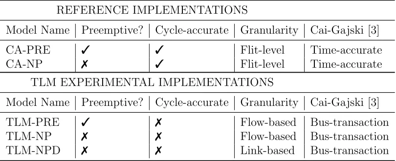
are the experimental TLM models evaluated here. Table 1 summarises the

key characteristics of these models. Criteria used for classifying the

mod-els include their priority preemption behaviour (priority preemptive or

non-preemptive), their cycle-accuracy (whether they function as a reference or

an experimental test model) and, for the TLM models, their granularity of

modelling. The granularity of modelling refers to whether the models store

and use individual link state in their NoC modelling decisions, or whether the

complete flow and its associated source-destination route is the fundamental

abstraction.

The relationship of the models to Cai and Gajski’s TLM classification [3]

is also defined in Table 1. The reference models CA-PRE and CA-NP are

(18)

model, in that they provide a cycle-accurate model of communication but an

abstraction of computation on the processing elements. The TLM-PRE,

TLM-NP and TLM-NPD models are examples of bus-transaction models,

in that they also approximate communication timings using the mechanisms

defined in Sections 5.4, 5.5 and 5.6.

REFERENCE IMPLEMENTATIONS

Model Name Preemptive? Cycle-accurate Granularity Cai-Gajski [3]

CA-PRE 3 3 _Flit-level _{Time-accurate}

CA-NP 7 3 _Flit-level _{Time-accurate}

TLM EXPERIMENTAL IMPLEMENTATIONS

Model Name Preemptive? Cycle-accurate Granularity Cai-Gajski [3]

TLM-PRE 3 7 _Flow-based _{Bus-transaction}

TLM-NP 7 7 _Flow-based _{Bus-transaction}

[image:18.612.111.516.250.415.2]

TLM-NPD 7 7 _Link-based _{Bus-transaction}

Table 1: The characteristics of the NoC models

Throughout the paper, the concept of flows is employed. A flow is

de-fined as a sequence of associated flits from the same source and destination

which travel together to their destination. Flows have an associated route,

which represents the links that they traverse on the route to their

destina-tion. Packets therefore represent the simplest example of a flow (being the

complete sequence of flits including a header and all transmitted data),

al-though a flow can also represent a partial packet which has not completely

entered its final flit into the NoC. All the TLM models presented track the

(19)

of the header flit of the packet along its route from the source node to its

destination. Flit position is required in the tracking of power consumption as

well as latency, since it provides information on the position of individual flits

relative to the links upon the route it traverses. Consider the progress of a

single packet under transmission from source to destination via intermediate

routers in an otherwise idle NoC, as shown in Figure 2.

Src

_R

_Dst

0

R

1

R

2

R

3

0 Src

2

2 R

₀

1 R

₁

0 R

₂

R

₃

_Dst

0 Src

1 R

₀

0 R

₁

R

₂

R

₃

_Dst

Src

_R

_Dst

0

2 R

1

1 R

2

0 R

3

3 Src

4 R

₀

3 R

₁

2 R

₂

1 R

₃

0 _Dst

Src

R

₀

R

₁

R

₂

R

₃

_Dst

Src

R

₀

R

₁

R

₂

R

₃

_Dst

2

1

3

4 Src

R

₀

R

₁

R

₂

4 R

₃

3 _Dst

Src

R

₀

R

₁

R

₂

R

₃

4 _Dst

2

3

4

T

i

m

e

[image:19.612.133.481.264.636.2]

Link index along route to destination

(20)

Potential values for flit position at a given time are in the range 0≤Fp < N+H−1,

in which the hop count of the route is given by H and N refers to the total

number of flits (including header flits) that the packet contains. A growing

phase occurs when Fp < H −1, in which data flits are in progress to the

destination, but some links further along the route can be idle as data flits

have not yet reached them. Following completion of the growing phase, every

link on the route has transmitted a header flit for this flow, and the

worm-hole process can continue to operate normally. The flow finally experiences

a shrinking phase in which Fp ≥ N. In this phase no additional data flits

are being injected, but the final flits are still in progress and have not yet

reached their destination. During transmission in the example in Figure 2

this flow goes through flit positions from 0 to 8 at successive time intervals.

5.2. CA-PRE - Preemptive Cycle-Accurate

The first model considered is a preemptive cycle-accurate model, referred

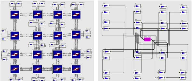
to as CA-PRE (Figure 3a). The figure shows the implementation of a test

NoC within the Ptolemy II simulation environment [28].

The CA-PRE model is structured to represent NoC components such as

arbiters, buffers and their associated ports as entities within the simulator.

On each transmission of a flit from one network component to another,

sim-ulator events have to be scheduled in order to process the arriving flit. For

example, flits arriving at an arbiter go through a simulated arbitration

(21)

virtual channels) which processes the virtual channels in priority order, and

ensures that the highest priority requesting arbitration is sent out upon the

relevant output port. Priority sorting ensures that each output port is only

used once for transmission per cycle, and port multiplexing state is tracked to

model the arbitration delays. Credit based flow control is used to control the

propagation of data through the network, allowing additional flits to enter

input buffers as they empty.

Delays are defined and timing information is tracked such that the

propa-gation of flits through the system is cycle accurate, but due to the requirement

for simulation events to model the propagation of each flit through multiple

simulation entities such as arbiters and buffers, time consumed in simulation

scales in proportion to the amount of data sent. This model is therefore used

as a reference implementation to validate the execution time performance

and accuracy of the TLM-PRE TLM model for preemptive NoCs. Although

the current implementation uses the Ptolemy II simulation environment, the

model structure is sufficiently generic to be applied to any simulator that has

objects with state, and port connections between them that trigger events

upon message arrival.

5.3. CA-NP - Non-preemptive Cycle-Accurate

The second model considered is a non-preemptive cycle-accurate model,

referred to as CA-NP. The fundamental structure of the CA-NP model at

(22)

(a) CA-PRE cycle-accurate simulation model (peer to peer NoC router topology)

[image:22.612.114.512.135.304.2]

(b) TLM-PRE TLM simulation model (entire NoC as single central entity)

Figure 3: The implementations of the simulation models for CA-PRE and TLM-PRE

within the arbitration code, in that their ports do not model the independent

buffering provided by virtual channels. In the alternative non-preemptive

design employed instead, the first flit to use a particular output port locks

that input-output port combination until the transmissions have finished.

All other requesting flows awaiting transmission on that output port of the

arbiter are blocked until completion of the in-progress flow, and therefore

cannot access the output port requested regardless of their priority level.

However, the fact that the input ports are processed in priority order ensures

that when two flows contend simultaneously for an output port, the priority

(23)

5.4. TLM-PRE - TLM Preemptive Single-Flow Activity

The TLM-PRE TLM preemptive model presented in this section is

de-scribed more fully in [4], [5] and [29]. The goal of the algorithm is to simulate

a priority preemptive NoC with a greatly reduced frequency of events. Events

are only processed upon flows entering or exiting the interconnect, or at

an-ticipated completion times for existing flows, in which simulation state must

be updated to ensure consistency. In the implementation of this and the

other TLM algorithms, an abstraction of the entire NoC is represented as a

single simulation entity (depicted centrally in Figure 3b). All abstractions of

processing elements are directly connected to this Interconnect entity.

The TLM-PRE algorithm is presented in Listing 1. The algorithm

oper-ates upon the set of currently active flows, processing them in priority order.

The algorithm uses the concept of interference sets in defining contention

between flows:

Definition 5.1. The interference setof f lowi is composed of flows of higher

priority than f lowi with routes sharing at least one link with the route of

f lowi. Flows are considered to be in the interference set regardless of whether

flits from an interfering flow request arbitration on those shared links

simul-taneously with f lowi.

For a particular f lowi, the algorithm tracks its current activation status

activei, and its remaining flits for transmission f litstosendi. During the

(24)

time tai. Completed flows are removed from the flow table. Activation of

any flows in the interference set of f lowi inactivates f lowi, preventing it

from transmitting. Flows without any active members of their interference

set are activated. Iteration over the flow set proceeds in priority order from

the highest to the lowest, ensuring that the activation decisions respect flow

priority. A further update event is scheduled at the expected completion

time of f lowi. Therefore, simulation events only occur when flows enter or

leave the NoC, or to update state at an expected flow completion time.

The trackPower function (Listing 2) is responsible for dynamic power

consumption modelling for a particular flow. It allows dynamic power

con-sumption of multiple flits to be tracked in a single simulator event, over a

time window in which it was known that the flow had exclusive access to

particular links. The trackPower function is invoked in two circumstances

during the update function; when f lowi completes, or when another higher

priority flow inactivates f lowi.

The trackPower function operates as follows. Firstly, the flowing time

can be computed by subtracting the current time from its last activation

time. The number of flits transmitted over this flowing time is computed

us-ing the flow’s flit transmission rate, which is by default assumed equal to the

system clock speed. A range of flits between startF litP os and endF litP os

is therefore determined. Iterating over both flit position and link index upon

the route, the flits which crossed a link are looked up from the flow’s

(25)

Listing 1: Pseudocode for updating a list of flows with power tracking (from [5])

1 update ( currentTime ) {

2 f o r each f lowi i n f l o w l i s t {

3 i f (activei) {

4 f litstosendi = f litstosendi − s e n t F l i t s ( currentTime −

tai) ;

5 tai = currentTime ;

6 i f (f litstosendi == 0 ) {

7 remove f lowi from f l o w l i s t ;

8 trackPower (f lowi) ;

9 }

10 f o r each f lown i n interf erencei {

11 i f (activen) {

12 activei = f a l s e ;

13 trackPower (f lowi) ;

14 }

15 }

16 } e l s e {

17 i f ( ! a c t i v e n f o r a l l f lown i n interf erencei) {

18 activei = t r u e ;

19 r e q u e s t U p d a t e ( currentTime + b a s i c L a t ( f l i t s t o s e n d i ) ) ;

20 }

21 }

22 }

(26)

Listing 2: Pseudocode for TLM dynamic power tracking (from [5]) 1 trackPower (currentF lowi) {

2 f lowing time = currentTime − tai;

3 endF litP os = startF litP os + f lowingtime ∗

f l i t T r a n s m i s s i o n R a t e (currentF low i) ;

4 f o r (f lit index = s t a r t F l i t P o s t o endF litP os) {

5 f o r (link index = 0 t o hopLength (currentF low i) ) {

6 f lit f or link = f lit index − link index;

7 i f (f lit f or link >= 0 and

8 f lit f or link < e n d F l i t L i m i t (currentF low i) ) {

9 link = g e t L i n k ( c u r r e n t F l o w i , link index) ;

10 f lit = g e t F l i t (f lit f or link) ;

11 r e g i s t e r T r a n s m i s s i o n (link, f lit) ;

12 }

13 }

14 }

15 s e t F l i t P o s (currentF lowi, endF litP os) ;

(27)

registerTransmission. This function handles dynamic power consumption

tracking for a particular flit and link, by tracking and accumulating bit

tran-sitions between sequential flits using a particular link. Since the algorithm

iterates over flit indices in its outer loop and along the route links in its inner

loop, the power consumption impact of previous flits will have been registered

in advance. It is therefore possible to extend the present work to apply more

advanced power models which incorporate cross-coupling between adjacent

links, e.g. [30] [31].

The example in Figure 2 shows a particular example of power

track-ing execution. Ustrack-ing a conventional cycle-accurate model in which every flit

transmission is directly modelled using low-level simulation events, simulator

events would be required upon every grey arrow. The TLM power tracking

described is able to model every flit transmission depicted with a single

simu-lation event, as long as the flow is not preempted during transmission. In the

case of preemption, an additional simulation event would be required, which

would handle modelling the completed flits up to the preemption point.

Consider Figure 2 to represent the algorithm’s internal processing.

Mov-ing from left to right along the horizontal axis (modelled in the inner loop of

Listing 2) represents advancing flits in single steps along their route to their

destination, with each gray arrow representing a power registration event for

a single flit. The rows represent sequential time-steps, which are handled in

the outer loop of Listing 2. Therefore, the link from processing core Src to

(28)

reg-istration. No link activity is modelled upon the vacant links closest to the

destination for flit positions 0 to 3, since the flow is still in its growing phase

and its flits have not reached this point yet. Correspondingly, the shrinking

phase occurs when the links closest to the source are idle.

5.5. TLM-NP - TLM Non-Preemptive Single-Flow Activity

In a preemptive NoC, it is always possible for a newly arriving higher

pri-ority flow to preempt another transmission in progress. The TLM simulation

model presented in this section, referred to as TLM-NP [6], operates upon

non-preemptive NoCs which do not permit such preemption. Upon flow

ad-mission, flows calculate their interference sets and activation status with any

other flow, in order to determine which flows will potentially interfere.

The pseudocode for the TLM-NP algorithm is the same as the previously

described TLM-PRE (Section 5.4), with a modification to the sorting order.

Instead of sorting flows for processing in order of priority, flows are sorted

on their distance to the next contention point (the link in the NoC at which

the routes of the two flows intersect). Priority is used as a secondary sorting

criterion if the distances to the next contention point are equal. For example,

two simultaneously arriving flows which wish to use the same link are sorted

such that the closest one to the contending router is processed first. Priority

is used as a tiebreak if their arrival at the point of contention would be

simultaneous. During the update event the flow processed first will reach the

(29)

passed through the contention point, then the model assumes that it cannot

be preempted and will flow until its f litsT oSendis zero.

5.6. TLM-NPD - TLM Non-Preemptive Dynamic Link Claiming

When one or more flows which share a link in common are active in the

network simultaneously, the TLM simulation algorithms presented in the

pre-vious sections have only allowed one of the them to be active simultaneously.

This may result in the simulation producing overestimates of latency, since

the model is too conservative in the temporal separation it provides. In the

real hardware implementation of a non-preemptive wormhole switching NoC,

both flows could advance through the arbiters along their routes in parallel,

until the latest of the two reaches the arbiter at which they are blocked or

contend for an output port. In the case of simultaneous arrival at an arbiter,

flow priorities would determine which would receive arbitration.

The TLM-NPD model is introduced in order to compensate for this, by

allowing individual links upon the route to be claimed dynamically. The

TLM-NPD model is the most sophisticated presented within this work, since

it models this situation by allowing multiple flows upon intersecting routes

to proceed simultaneously, claiming the links upon their arbiters up until the

point at which they will be blocked. This is therefore much more likely to

accurately predict latency in the problem case defined in Figure 1.

An earlier form of this non-preemptive NoC model (TLM-NPD) was

(30)

im-prove latency prediction performance under contention, by restricting flow

advancement during the growing phase to a single flit at a time. By contrast,

when a number of growing flows existed which attempt to request access to

multiple links, the early version of the algorithm described in [17], would

advance system time in a single operation, granting access to the contended

links to whichever flow was selected. This selection criteria was based on a

criterion of dominance, which considered flit positions to calculate distances

to the first contention point, as well as priorities. The dominance ordering

was computed up front and used as a sorting order. The necessity to

ad-vance system time in relatively course steps while assigning dominance in

this form produced problems in accurate link claiming prediction in complex

scenarios, when high contention lead to multiple blocking events occurring

over the update interval. The dynamic flow advancement in single flit steps

in the algorithm presented here as TLM-NPD solves this problem.

The increased reliance upon dynamic calculations means that the logic

for flow admission using in TLM-NPD is simplified. Upon admitting a flow

to the NoC, it is merely added to the flow table. Route intersection checking

or interference set (Definition 5.1) calculation is no longer required during

flow admission, since the dynamic flow move calculation during the update

events replaces them. The simulation now uses a time window start

lastUp-dateTime which records the time over which the interval should be

recon-structed. During flow admission, if no other flows are present in the system,

(31)

Listing 3: Pseudocode for the TLM-NPD algorithm: update of a list of flows 1 update ( currentTime ) {

2 i n t a r b i t e r P l u s L i n k P e r i o d s = a r b i t e r P e r i o d s + 1 ;

3 double time = lastUpdateTime ;

4

5 while ( time <= currentTime ) {

6 // P r o c e s s f l o w s s o r t e d i n p r i o r i t y o r d e r 7 f o r e a c h (f lowi s o r t e d by p r i o r i t y ) {

8 i f (f lowi. isGrowing ( ) ) {

9 headLink = f lowi. h e a d L i n k A t F l i t P o s i t i o n ( ) ;

10 i f ( headLink != n u l l and ! headLink . i s C l a i m e d ( ) )

11 tryGrowAdvance (f lowi, time , headLink ) ;

12 } e l s e tryFlowAdvance (f lowi, time ) ;

13 }

14 time += minFlowPeriod ( ) ;

15 }

16

17 lastUpdateTime = currentTime ; 18

19 f o r e a c h (f lowi s o r t e d by p r i o r i t y ) {

20 i f ( (f lowi. f l i t P o s i t i o n F i n i s h e d ( ) ) ) {

21 removeFlow (f lowi, currentTime ) ;

22 } e l s e {

23 completionTime = f lowi. timeToCompletion (

currentTime , a r b i t e r P l u s L i n k P e r i o d s ) ; 24 scheduleUpdateAt ( completionTime ) ;

25 }

26 }

(32)

Listing 4: Pseudocode for the TLM-NPD TLM function tryGrowAdvance 1 tryGrowAdvance (f lowi, time , headLink ) {

2 i f ( time >= (f lowi. lastMoveTime+minFlowPeriod ( )∗

a r b i t e r P l u s L i n k P e r i o d s ) ) {

3 // Claim i t

4 headLink . c l a i m L i n k (f lowi, time ) ;

5 // Move f o r w a r d s one , u p d a t e move time , t r a c k power

6 moveForwardTrackPower (f lowi, 1 , time ,

currentTime ) ;

7 }

Listing 5: Pseudocode for the TLM-NPD TLM function tryFlowAdvance 1 tryFlowAdvance (f lowi, time ) {

2 i f ( time >= (f lowi. lastMoveTime + f lowi. f l o w P e r i o d )

) {

3 // Move f o r w a r d s one , u p d a t e move time , t r a c k power

4 moveForwardTrackPower (f lowi, 1 , time ,

currentTime ) ; 5

6 i f (f lowi. i s S h r i n k i n g ( ) ) {

7 // Flow t a i l l i n k s can be r e l e a s e d 8 t a i l L i n k = f lowi. t a i l L i n k ( ) ;

9 i f ( t a i l L i n k != n u l l ) {

10 t a i l L i n k . r e l e a s e L i n k (f lowi, time ) ;

11 }

12 }

13 }

(33)

The pseudocode for update is presented in Listing 3. The first section

of the algorithm operates differently to the other TLM algorithms, in that

it is based upon advancing all flows simultaneously through the network in

single-flit steps as blocking permits, rather than computing the maximum

move limited by time and then advancing the flow in a single operation.

This is necessary in order to accurately model the claiming and releasing of

link locks when shorter flows are present in the network, since the release

of the lock upon a link may allow another flow behind it to advance. The

outer loop of the algorithm between lines 5 and 15 advances time forwards

in increments of the minimum processing period of flows in the network (by

default, this is equal to the system clock speed). The inner loop in lines 7

to 13 iterates over all active flows in priority order. This priority-ordered

iteration ensures that the all the higher priority flows in a flow’s interference

set (Definition 5.1) have been considered to check if they are eligible to claim

a link under contention, which respects the priority-favouring design of the

real hardware system.

If the flow is in its growing phase (in which it has not yet acquired all

the necessary links on the route to its destination), then the next link that

will be required by the advancing head is tested to determine if it is free

or claimed. If it is free, then tryGrowAdvance (Listing 4) is executed. This

compares the iteration time with the time of the flow’s next permitted move,

in order to determine if it can proceed yet. If this condition is met, then

(34)

consists of claiming the relevant link at the head. This is followed by (in the

function moveForwardTrackPower) incrementing the flow flit position, and

tracking the power impact of registering the single flits in one move.

If the flow is not in its growing phase (that is, its header has claimed

all the links to its destination) then it is immune to blocking given that the

NoC design assumed is non-preemptive. Therefore,tryFlowAdvance (Listing

5) is called to determine whether the flow can move forward. tryFlowAdvance

verifies that the time elapsed since the last move is equal to or greater than

the flow processing period, and if so advances the flow. If the flow is in its

shrinking phase, then it is also necessary to free the link at the tail every

time it moves forwards.

The last step for update in lines 17 to 26 of Listing 3 is to register the

time of this last update, and to work out which flows have completed and

which need to be scheduled for further processing. Accordingly, the code

iterates over all flows within the network, testing their flit positions to

deter-mine whether these flows have already completed. If they have completed,

then they are removed from the network. If not, then their estimated

com-pletion time (assuming no further blocking events occur) is computed. An

additional update is scheduled at this time in order to handle their remaining

transmissions.

One particular issue involved that may produce inaccuracies in the

TLM-NPD model is consideration of buffering in the network. In the reference

(35)

attached to particular input ports (one buffer per virtual channel in the

priority-preemptive NoC). This allows several flits to be stored within one

arbiter input buffer, which can produce a bunching up of multiple flits at

intermediate buffers. However, for modelling simplicity, the concept of flit

position used for the TLM models assumes that all flits are arranged

sequen-tially along their respective route, without bunching up within the buffers of

intermediate routers. This therefore can lead to some incorrect predictions

of flit position and the resulting preemption behaviour by the TLM models,

as examined in the results.

6. Results

This section presents simulation results to evaluate the simulation

execu-tion time performance, latency and power consumpexecu-tion modelling accuracy

of the various TLM models compared to the cycle-accurate reference. The

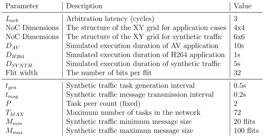
default parameters used throughout the simulations are given in Table 2. If

alternatives to these default parameters are used in any particular simulation

run, it will be specified during the description of the particular experiment.

6.1. Simulation Execution Time Performance Results

A major issue for NoC simulations is improving their overall execution

time while retaining accuracy, in order to allow realistic application cases

to be simulated. This subsection considers the wall-clock execution times of

(36)

Parameter Description Value

Larb Arbitration latency (cycles) 3

NoC Dimensions The structure of the XY grid for application cases 4x4 NoC Dimensions The structure of the XY grid for synthetic traffic 6x6

DAV Simulated execution duration of AV application 10s

DH264 Simulated execution duration of H264 application 1s

DSY N T H Simulated execution duration of synthetic traffic 5s

Flit width The number of bits per flit 32

tgen Synthetic traffic task generation interval 0.5s

tmsg Synthetic traffic message transmission interval 0.2s

P Task peer count (fixed) 2

TM AX Maximum number of tasks in the network 72

Mmin Synthetic traffic minimum message size 20 flits

[image:36.612.108.532.127.345.2]

Mmax Synthetic traffic maximum message size 100 flits

Table 2: Parameters for the overall simulation methodology, and for synthetic traffic generation

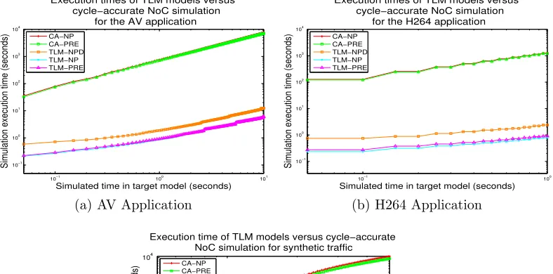
against reference cycle-accurate models for the three application cases

consid-ered. Figure 4a illustrates the execution time performance of the TLM and

reference models for the AV application, indicating that the simpler TLM-NP

model is approximately 3.1 orders of magnitude faster than cycle-accurate.

The TLM-NPD algorithm is approximately 2.7 orders of magnitude faster.

This relative reduction in speed for TLM-NPD compared to TLM-NP occurs

due to the requirement for the TLM-NPD algorithm to iterate in a nested

loop forwards over the time window and also over all active flows, which is

more time-consuming than the logic of TLM-NP. Considering the

preemp-tive models for the AV application, the TLM-PRE algorithm has effecpreemp-tively

(37)

10−1 100 101 10−1 100 101 102 103 104

Simulation execution time (seconds)

Simulated time in target model (seconds)

Execution times of TLM models versus cycle−accurate NoC simulation

for the AV application

CA−NP CA−PRE TLM−NPD TLM−NP TLM−PRE

(a) AV Application

10−1 100 10−1 100 101 102 103 104

Simulated time in target model (seconds) Execution times of TLM models versus

cycle−accurate NoC simulation for the H264 application

(b) H264 Application

100 10−1 100 101 102 103 104

Simulated time in target model (seconds)

Execution time of TLM models versus cycle−accurate NoC simulation for synthetic traffic

[image:37.612.117.511.141.336.2]

(c) Synthetic Traffic

Figure 4: Performance of the transaction-level model simulations compared with a cycle-accurate reference model

both algorithms are very similar. Similarly, the preemptive cycle-accurate

reference PRE displays very similar execution time performance to

CA-NP, since their simulation structure and event counts are very similar.

Figure 4b illustrates the execution time performance of the H264

applica-tion. The simulation duration is much shorter, and there is a smaller increase

(38)

applica-tion produces lower contenapplica-tion. The TLM-NP and TLM-PRE models exhibit

3.1 orders of magnitude execution time performance improvement over the

CA-NP and CA-PRE cycle-accurate simulations. The TLM-NPD model

de-livers 2.7 orders of magnitude improvement. The vertical steps shown in the

results arise due to the staggered release of packets from the central

trig-gering clock of the H264 application, which produces variations in network

loading at different sampling intervals.

Figure 4c illustrates the equivalent execution time performance for the

synthetic traffic generator, starting with the injection of the first tasks into

the system. Since tasks are generated dynamically for this simulation starting

with an empty network, at the beginning of the simulation model-independent

features such as simulation setup, data generation and packet generation are

dominant over the modelling of simulation transmission events. Therefore,

at the start the execution timing performance advantage of the TLM

simula-tions over cycle-accurate is comparatively low. However, as additional tasks

are generated as simulation execution progresses, the load placed upon the

NoC and total flit transmission rate throughout the NoC increases. Since

the cycle-accurate models require simulation events per every flit

transmit-ted, the advantage of the TLM models becomes greater, producing

approxi-mately 3.3 and 3.1 orders of magnitude timing performance improvement for

the TLM-NPD and TLM-NP models over cycle-accurate. As in the AV

ap-plication case, TLM-PRE provides an equivalent execution time performance

(39)

6.2. Latency Accuracy

The communication latencies produced during simulation by the TLM

models will vary according to how their algorithms handle the contention

between flows. This section presents and compares the normalised

laten-cies delivered for preemptive and non-preemptive TLM simulation models,

grouping packets according to their priorities. Normalised latency refers to

the latency per flit, that is, the total communication latency divided by the

number of flits transmitted. The total latency experienced by a packet

dur-ing transmission depends on the contention experienced durdur-ing transmission,

which may change due to the activities of other flows at the transmission

in-terval. Therefore, a maximum-minimum range is specified at each priority

level. Priorities are defined so that the low priority index values represent

the highest priorities (e.g. priority 1 is therefore the highest priority in the

system). All packets transferred between a source-destination pair in the

application model use the same priority.

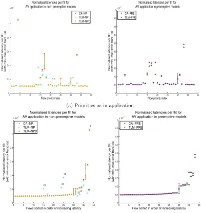
The latencies for the autonomous vehicle application are considered in

Figure 5a, covering results occurring over 10 seconds of simulation runtime.

The results show that the accuracy of the TLM-NPD algorithm is

over-all very high, with the largest error in the maximum normalised latency

under-estimation upon flow priority 17 corresponding to 15 flit-times (0.25

flit-times per message flit, with a message size of 60 flits). By contrast the

TLM-NP model exhibits large latency errors in several flow priorities,

(40)

0 5 10 15 20 25 30 35 40 0 0.2 0.4 0.6 0.8 1

x 10−7

Flow priority index

Normalised latency per flit

(with min−max error bars) (s)

Normalised latencies per flit for AV application in non−preemptive models

CA−NP TLM−NP TLM−NPD

0 5 10 15 20 25 30 35 40

0 0.1 0.2 0.3 0.4 0.5 0.6 0.7 0.8 0.9 1x 10

−7

Flow priority index

Normalised latencies per flit for AV application in preemptive models

CA−PRE TLM−PRE

(a) Priorities as in application

0 5 10 15 20 25 30 35 40

0 0.2 0.4 0.6 0.8 1

x 10−7

21 31

14

2215 33

4

Flows sorted in order of increasing latency

Normalised latencies per flit for AV application in non−preemptive models

CA−NP TLM−NP TLM−NPD

0 5 10 15 20 25 30 35 40

0 0.1 0.2 0.3 0.4 0.5 0.6 0.7 0.8 0.9

1x 10

−7

Flow sorted in order of increasing latency

Normalised latencies per flit for AV application in preemptive models

CA−PRE TLM−PRE

[image:40.612.114.506.159.576.2]

(b) Flows sorted in latency order

(41)

33. This occurs since the simpler TLM-NP algorithm in incapable of

track-ing precisely where contention occurs durtrack-ing the progression of a flow durtrack-ing

its growing phase. In the preemptive case, the TLM-PRE algorithm is more

accurate, since a preemptive architecture is inherently more predictable in its

timing. The only flow priority for which the latency is particularly

inaccu-rate is 19, in which there is an underestimate since the TLM-PRE algorithm

cannot model accurately contention during the growing and shrinking phases

of routes, conservatively assuming the route is active throughout. Figure 5b

shows the flows from the same simulation rearranged in order of increasing

mean normalised latency (in the cycle-accurate reference model), to

demon-strate the general trend in TLM simulation accuracy for flows with increasing

contention.

For the TLM-PRE algorithm for the AV application case, the normalised

latencies are overall a closer match to the cycle-accurate case, since the

sce-nario is overall more predictable. The largest latency error occurs for

prior-ity 19, in which the normalised latency is approximately 66% higher for the

cycle-accurate reference.

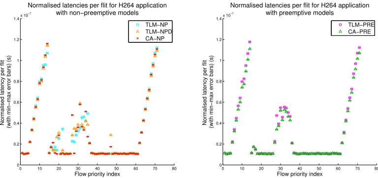
For the H264 application (Figure 6) in the non-preemptive case, both

TLM-NP and TLM-NPD correctly model overall structure of the latency

’ramp-up’ effect with priority that exists for low and high priorities. This

feature of the application arises as a result of the fan-out inherent in two

places in the H264 application, in which one source task transmits

(42)

0 10 20 30 40 50 60 70 80 0 0.2 0.4 0.6 0.8 1 1.2 1.4x 10

−7

Flow priority index Normalised latency per flit _{(with min−max error bars) (s)}

Normalised latencies per flit for H264 application with non−preemptive models

TLM−NP TLM−NPD CA−NP

0 10 20 30 40 50 60 70 80

0 0.2 0.4 0.6 0.8 1 1.2 1.4x 10

−7

Flow priority index Normalised latency per flit _{(with min−max error bars) (s)}

Normalised latencies per flit for H264 application with preemptive models

[image:42.612.113.497.126.307.2]

TLM−PRE CA−PRE

Figure 6: Latency results for the H264 application under both preemptive and non-preemptive models

simultaneous application release, the model is very sensitive to cascading

latency errors, and for both TLM-NP and TLM-NPD there are two

trans-missions that are predicted incorrectly (priority 22 for TLM-NP and priority

28 for TLM-NPD). For the H264 preemptive case, the overall application

structure is more predictable since the NoC is preemptive and there is less

dependence on exact details of timing. This produces lower errors between

TLM-PRE and the CA-PRE cycle-accurate reference.

For the synthetic traffic simulations, results are displayed using flow

re-sorting (in order of increasing mean cycle-accurate latency) only. Since the

flow priorities are randomly selected and there is no defined application

struc-ture to the network, flow patterns are difficult to process intelligibly without

resorting. Figure 7 displays the resorted normalised latency of flows. For the

(43)

markers in addition to the NP data series. It is clear that the

TLM-NP algorithm provides a very poor estimate of latency in the non-preemptive

case, in that there is no relation between the shape of the cycle-accurate curve

and the TLM model. This occurs since the synthetic traffic produces much

higher contention than the other application examples, given that the task

peering relationships and mappings are randomly generated. Many flows

are blocked two or more times during their growing phase, which given the

wide variety of flow lengths and mappings can produce normalised latencies

per flit up to five times higher, or twice as low as the cycle accurate

(CA-NP) reference. By contrast, TLM-NPD provides much closer estimations

of cycle-accurate latency, with an overall close correspondence between the

mean values for TLM-NPD and the cycle-accurate reference. This is due

to its ability to track the timings and advancements of flows and therefore

anticipate which flow will receive arbitration in the event of a small timing

offset.

In the CA-PRE and TLM-PRE model comparison, it is notable that in

most cases the TLM model produces a latency above the reference

cycle-accurate model. However, occasionally the minimum latency is below the

minimum latency of the cycle-accurate reference. This can occur due the

dependencies between flows, in which a latency prediction error for one flow

in the TLM model can cause a dependent flow to miss contention that would

(44)

0 20 40 60 80 100 120 140 0.2 0.4 0.6 0.8 1 1.2 1.4 1.6 1.8

x 10−7

Flows sorted by mean normalised latency Normalised latency per flit _{(with min−max error bars) (s)}

Normalised latencies per flit for synthetic traffic with non−preemptive TLM models

TLM−NP TLM−NPD CA−NP

0 20 40 60 80 100 120 140

0.2 0.4 0.6 0.8 1 1.2 1.4 1.6 1.8

x 10−7

Flows sorted by mean normalised latency Normalised latency per flit _{(with min−max error bars) (s)}

Normalised latencies per flit for synthetic traffic with preemptive TLM models

[image:44.612.119.498.123.307.2]

CA−PRE TLM−PRE

Figure 7: Latency results for synthetic traffic under both preemptive and non-preemptive models

6.3. Worst Case Latency Errors

As a summary, the maximum worst-case normalised latencies (per-flit

latency) errors generated by the various TLM models are presented in Table

3. These errors are computed by comparing the peak normalised latency

produced a TLM model against the latency produced by the relevant

cycle-accurate model. The priority level which produced the latency error is also

annotated.

It is notable that considering the non-preemptive cases, the TLM-NPD

model is significantly more accurate than the TLM-NP model predictions in

the AV application and synthetic traffic cases. Particularly in the synthetic

traffic case, there are a large number of priority levels which produce a high

relative error for TLM-NP (as depicted in Figure 7) in addition to the worst

(45)

mapping and the significant admission of packets to multiple destinations,

the worst case normalised latencies of the two models are approximately

equal.

Application TLM-NP TLM-NPD TLM-PRE

AVApp -74.3% (priority 33) -5.2% (priority 17) +66% (priority 19) H264 +218.0% (priority 22) +218.0% (priority 28) +39% (priority 28) Synthetic traffic +687% (priority 76) +32% (priority 29) +42% (priority 70)

Table 3: Maximum latency errors experienced by the TLM models

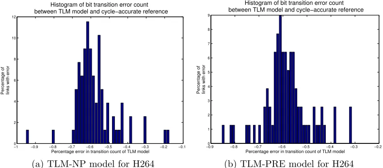
6.4. Link Transition Modelling Accuracy

This section considers the error in NoC link dynamic power consumption

modelling for the various TLM models, compared to the cycle-accurate

ref-erence. The dynamic power consumption on the links is approximated using

a model which counts the number of bit transitions upon the NoC links.

Although this does not include power consumption effects obtained from

switching logic or power coupling costs, due to the length of NoC links they

comprise a significant individual source of NoC dynamic power consumption

[18] [32] [21] [22] [19]. The results are presented as histograms indicating the

proportion of links in the network which exhibited the indicated error, which

allows the distribution of link errors to be examined.