On green pythons : the ecology and conservation of Morelia viridis

(1)

(2)

This is the book of David, the son of Abraham and the father of Jesus Christ Matthew 1.1

Declaration

This thesis is my original work and no part has been previously submitted for a degree. Chapters II, III and IV are in press and have been are co-authored with Rob Heinsohn, Sarah Legge, John Endler and Jeff Wood. I am, however, the principal contributor to these chapters.

(3)

On green pythons _iii

Abstract

The green python Morelia viridis is a most striking animal. Individuals are born either brick red or bright yellow and both colours change to green as adults. These colours and the remarkable colour change have long made them of interest to biologists and in demand for the pet trade. Despite this interest nothing is known of their

distribution, biology or ecology in the wild. Here I address this knowledge gap by presenting results from the first detailed study of the species, at Iron Range on eastern Cape York Peninsula, Australia.

Individual growth was described by the von Bertalanffy growth curve, with a maximum predicted size of 1.35 metres snout-vent length. Males matured at 2.4 years and females at 3.6 years, and growth was indeterminate after approximately 12 years. The colour change from yellow to green occurs at 55 centimetres, which corresponds to individuals approximately a year old. There was no sexual dimorphism in adults, however juvenile females had larger heads than juvenile males. Adult sized individuals comprised ~50% of the population.

Females had a home range of 6.2 ± 1.9 ha (mean ± SE), which was positively correlated with their snout-vent length. Males adopted a roaming strategy through suitable habitat while juveniles were restricted to areas where more light reached the ground. There was overlap between multiple female home ranges, and between female home ranges and the movement paths of males. There were no differences in the distances moved by males and females of any size, although the variation in movement distances was greater in the dry season than the wet season.

Green pythons are obligate ambush predators which eat a variety of prey. They show an ontogenetic shift from invertebrates and terrestrial, diurnal reptiles to birds and terrestrial, nocturnal mammals. This diet change is concurrent with a shift in the time of hunting, and the location and characteristics of ambush sites. Yellow individuals were usually found within ten metres of the ground, while green individuals used the full vegetation strata and were often found in the canopy.

The three colour morphs of the green python appear to be adaptive for

(4)

morph in only the canopy, where it was half as conspicuous as either the red or yellow morph. In both leafy and non-leafy sub-canopy environments green individuals were more conspicuous than both yellow and red morphs. Red morphs were least

conspicuous in only the non-leafy sub-canopy environment. The conspicuousness of green males decreased with age, but this was not the case with green females. Predation of plasticine models of the three colour morphs showed that red models were ten times more likely to be predated than either green or yellow morphs, however the model colours did not always match the real morph colours.

(5)

On green pythons _v

Acknowledgements

If I have seen farther than others, it’s because I’m standing on the shoulders of giants.

Me (and Sir Isaac Newton)

Firstly I would like to thank my supervisor, Rob Heinsohn. He provided the inspiration for this project, and his suggestions and support throughout these four years have made this project better than otherwise possible. He has also become a good friend, and I can’t imagine a better person with whom to work.

Many people assisted in some capacity during fieldwork. I would especially like to thank Peter Barrett & the staff of the Marlin Coast Veterinarian Clinic, Andrea Cook, Karl Goetze, Karl Hillyard, Nadine Kelly, Sarah Legge, Steve Murphy, Bess Schenk, Ellie Sobey and Kristie Wilson. I especially thank those that spent any time wandering around the rainforest at night with me. You may have saved me from my own sanity.

It was a pleasure to work in the Centre for Resources and Environmental Studies, and I met many very cool people here; Nadeena Beck, Caroline Blackmore, Adam and Annika Felton, Joern Fisher, Jake Gillen, Frank Jotzo, Adrian Manning, Nicki Munro, Phil Pagan, Glenn Sanecki, Kate Sherren, Jess Weir, Martin Worthy and Kara

Youngentob. Thank you for allowing me to distract you, beyond the call of duty.

Tim Mensforth of Ultimate Reptile Supplies in Adelaide and Tim Morris in the USA shared their considerable knowledge on captive breeding in the species. Karl Nissen provided helpful mapping advice, Jeff Wood invaluable statistical advice and John Endler discussions and thoughtful analysis of colour.

My family and friends have always provided unconditional support, even when they doubted my sanity. My parents - Anne and Kent – gave me the ability to do anything. Matt, Wendy, Karl and Bess, Nadine, Julia and Emma made the pain of fieldwork seem worthwhile as it allowed them to live vicariously. My time in Canberra has been so much fun thanks to the ‘extended family’ that is ultimate frisbee.

(6)

Figures

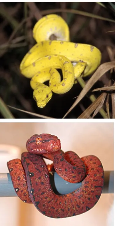
Figure 1. The three colour morphs of the green python. The red and yellow forms are juvenile, while all adults are green... 6 Figure 2. Predicted global distribution of the green python Morelia viridis. Location

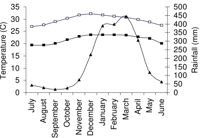
records for Australia and Papua New Guinea are based on climate modelling with known collection localities (see Chapter VI). Location records are incomplete for West Papua, hence the map is entirely shaded to indicate their likely distribution. 7 Figure 3. Map showing the location of the study area in northern Australia... 15 Figure 4. Environmental variables at Lockhart River airport (approximately 10 km

from the study site). Mean monthly minimum and maximum temperatures in degrees Celsius ( –minimum, – maximum) and mean monthly rainfall in millimetres ( ). Note the x-axis runs from July to June, rather than for the

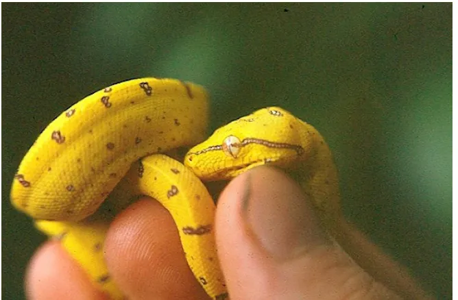
calendar year... 16 Figure 5. The smallest individual caught during fieldwork. Thirteen grams and 33

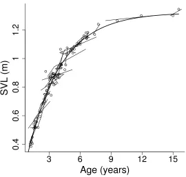
centimetres long... 18 Figure 6. Growth rate curve for the green python Morelia viridis at Iron Range based

on growth between recaptures of individuals. Open circles represent actual measurements, lines are the growth rate of individual pythons between captures and the smooth curve is the predicted relationship between age and size. ... 19 Figure 7. Size class distributions for the population of green python Morelia viridis at

Iron Range, Australia. See text for details on size class limits... 21 Figure 8. Relationships between the snout-vent length of individual green pythons

Morelia viridis at Iron Range and other morphometric variables measured; females – filled triangles and solid line; males – open nabla and broken line. All data has been transformed with natural logarithms. X – axis, snout-vent length.. 22 Figure 9. Frequency of SVLs (snout-vent lengths) recorded for all green python

Morelia viridis captures between 1999 and 2005 at Iron Range, Australia. ... 23 Figure 10. Individual in the process of changing colour from yellow to green. ... 24 Figure 11. Incremental area plots for Morelia viridis home ranges: (a) green males, (b)

green females, and (c) yellow individuals... 40 Figure 12. Home range areas of four radio-tracked individuals... 41 Figure 13. Predictions of the natural logarithm of distance moved for individual snakes

(10)

(yellow individual). ...52 Figure 15. Proportion of times hunting out of all location records. Proportions are

shown separately for sex and time of day...54 Figure 16. Perch heights for each size class of Morelia viridis at Iron Range National

Park, Australia during the day (black columns) and night (open columns). ...56 Figure 17. Relative frequency of locations for each green python size class that used the ground as perch substrate compared with above ground perches...57 Figure 18. The diameter of the perch for resting and hunting green pythons Morelia

viridis at Iron Range National Park. Females are shown as solid columns, males open columns. Error bars are standard errors of the differences. ...58 Figure 19. Disparity values for green pythons viewed by conspecifics (grey columns) or

by avian predators (black columns) in (a) the canopy, (b) the leafy sub-canopy environment or (c) the non-leafy sub-canopy environment. ...76 Figure 20. Comparison of the disparity between the three green python colour morphs

in locations where (a) yellow or (b) green individuals were found. ...77 Figure 21. The disparity of individual green pythons against their pooled backgrounds

as they increase in size. Values are means and standard errors as predicted by the best fitting linear mixed model. ...77 Figure 22. Percentage of each plasticine colour morph predated at Iron Range. Filled

columns; dry season, open columns; wet season. ...79 Figure 23. BIOCLIM prediction of climatically suitable areas for green pythons

Morelia viridis in Papua New Guinea. Light grey represents total range, while dark grey represents the predicted core range. Dots are the sighting locations on which the prediction is based...94 Figure 24. Predicted distribution of the green python in Australia: a) BIOCLIM

prediction of climatically suitable habitat. Light grey areas represent total range, while the dark grey area represents core range, b) prediction based on vegetation matching with known locations of green python sightings. Dots are sighting localities on which the predictions are based...95 Figure 25. Demographic composition of the green python population in the survey area.

(11)

On green pythons

4

Tables

Table 1. The evolutionary significance of ontogenetic colour change. Table adapted from Booth (1990). ... 30 Table 2. Individual green pythons Morelia viridis radio-tracked during this project ... 38 Table 3. Results for the generalized linear mixed model testing movement distances of

individual Morelia viridis. Terms were added sequentially to the fixed model.... 42 Table 4. Selected daily movement sequences for four Morelia viridis at Iron Range

National Park. ... 43 Table 5. Prey items recorded from green pythons during this study and from other

published records. Prey species were active diurnally (D) or nocturnally (N), snakes were either male (M) or female (F) and snake colour either yellow (Y) or green (G)... 59 Table 6. Known and potential predators of the green python Morelia viridis throughout

its distribution. ... 71 Table 7. Details of locations used in the BIOCLIM prediction of the distribution of

green pythons in Papua New Guinea. Locations are sourced from museum records, my surveys and O’Shea (1996)... 89 Table 8. Details of locations used in the BIOCLIM prediction of the distribution of

green pythons in Australia. Locations were primarily from my surveys, with additional locations from K. McDonald (pers. comm. 2003), S. Templeton (pers. comm. 2005), Waldren (1996) and Christian (1997)... 90 Table 9. Regional ecosystems categories where the green python Morelia viridis was

found in Australia, their dominant species and the extent of each regional

(12)

(13)

On green pythons ₅

General Introduction

“Wij maken nog gewag van eene andere nieuwe soort van de Aroe-eilanden, Python viridis, omdat zij in hare gestalte, haar zaemgedrukt ligchaam en hare groene met witte

vlekjes afgebrokene kleur, de grootste overeenkomst met Boa canina van Zuid-Amerika heeft”

“(We want to mention a different new species from the Aroe Islands, Python viridis, because her bodily shape, her compressed body and her green and white dotted colour,

hugely resemble the Boa canina of South America.)”

(Schlegel 1872)

Introduction

The green python Morelia viridis was first collected from the Aroe Islands, in the Dutch East Indies (now the Aru Islands of Indonesia) some time in the mid to late 1800s. It must have been a rare species even then as Alfred Russell Wallace, who spent considerable time in the Aru Islands never saw or collected a specimen (Wallace 1869). It was formally described by Schlegel (1872) at the Leiden Museum as Python viridis, in the genus Python due to its resemblance to other pythons known at the time, and with the specific name viridis due to the vivid green colour (the type specimen was obviously an adult). In 1874 Meyer re-examined green pythons and established the monotypic genus Chondropython, where it stayed until Kluge (1993) included it with Morelia.

(14)

[image:14.612.79.279.167.552.2]

patterns (Maxwell 2003). In the wild juveniles occur in two colour morphs – a bright yellow and a “brick” red, and both change to vivid green. The adaptive significance of such ontogenetic colour change and indeed colour polymorphisms in general is not well understood (Booth 1990; Galeotti et al. 2003; Hoffman & Blouin 2000).

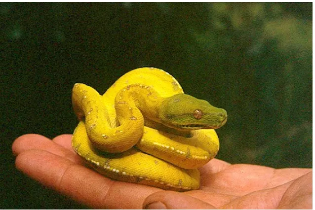
Figure 1. The three colour morphs of the green python. The red and yellow forms are juvenile, while all adults are green.

(15)

On green pythons ₇

‘The green python is a creature of the forest, coiled quietly on some arboreal perch or prowling through the trees and on the ground’ (Barker & Barker 1994).

“The green python is a nocturnal, arboreal python which normally shelters in tree hollows, epiphytic ferns, etc. during the day. Feeds on small mammals and birds” (Cogger 1996).

“...restricted to moist, closed forests....where it rests in a distinctive coiled posture on a horizontal branch or vine in dense vegetation. Green pythons use their tail tip to lure prey and to drink from pools that form in their coils after rain” (Torr 2000).

[image:15.612.161.508.313.578.2]

“This python forages on the ground at night. Sleeping specimens maybe located....in tree clefts, epiphytic plants and on low branches during the day. There is no evidence that birds form a significant part of their diet” (O'Shea 1996).

Figure 2. Predicted global distribution of the green python Morelia viridis. Location records for Australia and Papua New Guinea are based on climate modelling with known collection localities (see Chapter VI). Location records are incomplete for West Papua, hence the map is entirely shaded to indicate their likely distribution.

(16)

Papua New Guinea and Australia (Cogger 1996; O'Shea 1996) (Figure 2). In Indonesia they are found in West Papua including the Aru (Aroe) Islands and the islands of the Geevlink Bay (Biak, Yapen and possibly Numfor). In Papua New Guinea they are found on the mainland and the D’Entrecasteaux Islands, however they have not been recorded from New Britain or islands further east (O'Shea 1996). In Australia the species is limited to the Cape York Peninsula in Queensland (Cogger 1996).

Aims

The aims of this thesis are twofold. The primary aim is to gain a detailed understanding of the basic biology and ecology of the green python, its distribution and conservation status. Snakes are an understudied group of organisms when compared with mammals or birds mainly due to the relative difficulty involved in studying them. Despite these factors they are ideally suited to answering a variety of important theoretical and evolutionary questions (Shine & Bonnet 2000). In many instances the basic biology and ecology of snake species is unknown, limiting their applicability in answering broader questions. A detailed ecological understanding is also necessary to determine the conservation status of a species, and evaluate the potential effect of different threats on its survival. A species’ life history has important implications in all aspects of its biology, including longevity, survival and reproductive success (Chivers et al. 2001; Palkovacs 2003; Zuk & Stoehr 2002). Differences in the life history traits between individuals of a single species can lead to niche separation, and ultimately speciation if these differences are maintained over many generations (Luiselli 2006; Marzluff & Dial 1991). Variation in life history traits in snake species has long been of interest to scientists due to the wide variety of exhibited traits (Chiaraviglio et al. 2003; Fitch 1987; Shine 2005).

Here I establish the ecology of the green python, including population structure and dynamics, movements and feeding behaviour. The implications of these findings, along with their predicted distribution (from climatic and vegetation models) can then be used to assess the conservation status of the species.

(17)

On green pythons ₉

(Galeotti et al. 2003; Hoffman & Blouin 2000; Lank 2002). The evolutionary reasons underlying ontogenetic colour change are even less well understood (Booth 1990), and there have been few rigorous studies of this phenomenon in the wild (but see Graf and Nentwig (2001)).

Thesis structure

This thesis is organised into five data chapters. Each chapter is designed to stand alone and includes a thorough introduction to the specific topic of the chapter, and a review of relevant literature. All chapters are written in a style suitable for publication; three chapters are already in press. A brief outline of the thesis is as follows.

• Chapter I. General introduction.

• Chapter II. I establish the basic biological parameters for the population at Iron Range, Australia. This includes growth rates and aging, morphometric

characteristics, population structure and establishes the timing of ontogenetic colour change from yellow to green. This chapter has been accepted in the Journal of Zoology (London).

• Chapter III. I compare the movements of males, females and juveniles, testing for ranging behaviour, and determining daily distances moved and movement patterns. I also look for behavioural differences between the wet and dry seasons. This chapter has been accepted in Austral Ecology.

• Chapter IV. I detail the foraging ecology of individual green pythons, including detailed analyses of where and when they hunt. I include a list of all prey items recorded, and a measure of hunting success using time-lapse video footage. I also consider their behaviour when they are not hunting. This chapter has been accepted in the edited volume ‘The Biology of the Boas and Pythons’, Eagle Mountain Publishing (eds. R. Henderson & R. Powell).

• Chapter V. I examine the adaptive significance of the two juvenile colour morphs and the ontogenetic change to green using advanced techniques for analysing colour. These compare colour morphs with alternate possible habitat backgrounds “looking” through the eyes of both conspecifics and predators. • Chapter VI. I run a bioclimatic model to predict the green python’s distribution

(18)

likely distribution using regional ecosystem maps. At Iron Range I determined the density of individuals using surveys and capture-recapture techniques. I discuss the likely conservation status of green pythons using the density and demographic parameters attained in this study.

(19)

On green pythons ₁₁

Chapter II

Life history traits and ontogenetic colour change in an arboreal

tropical python,

Morelia viridis

(20)

Abstract

The Pythonidae are a widely distributed group of snakes that fill a variety of niches in Africa, Asia and Australasia. I used mark-recapture techniques to describe the life history traits and colour change in the green python Morelia viridis, an iconic species that is poorly known in the wild. Modelling of growth rates revealed that males and females reach sexual maturity after 2.4 and 3.6 years respectively, and are

predicted to live for at least 15 years. Extrapolation from small individuals revealed a highly seasonal breeding period with hatching in late November. However, few hatchlings were recorded in any one year suggesting that adults do not breed every year. The adult sex ratio did not statistically differ from parity, but immature females significantly outnumbered immature males. Approximately 50% of all snakes captured were adult-sized. Sexual dimorphism was not detected in the adults, but juvenile females have larger heads than juvenile males. Ontogenetic colour change from yellow to green occurred between 53 and 59 cm and, based on growth rates, occurs at

(21)

On green pythons ₁₃

Introduction

The pythons (Pythonidae) are a widely distributed family of approximately 24 species occurring in tropical, sub-tropical and temperate areas of Africa, Asia and Australasia (Greer 1997), and have been known for thousands of years (Charlesworth 2004). Pythons have radiated extensively, with species filling ecologically diverse niches from the desert to the tropical rainforest and aquatic ecosystems (Barker & Barker 1994). They range in size from the diminutive pygmy python Antaresia perthensis which reaches 47 cm (Shine & Slip 1990), to the giant reticulated python Python reticulatus of South East Asia which has been recorded close to 9m in length (Murphy & Henderson 1997).

Adult pythons are predominantly ambush predators of mammals, but some have specialised to feed on reptiles, birds, fish, frogs or invertebrates, and many show ontogenetic changes in diet (Greer 1997; Shine et al. 1998; Slip & Shine 1988a). In some areas pythons are an important ecosystem predator and can maintain very high densities (Groombridge & Luxmoore 1991; Shine et al. 1998; Shine & Madsen 1997). Pythons show remarkable variation in both body coloration and patterns between species, resulting in high demand from the captive pet trade and for skins for the leather industry. Some species may be threatened by the skin and captive pet trades

(Groombridge & Luxmoore 1991; Jenkins & Broad 1994), although the true extent of the problem is rarely known.

Green pythons Morelia viridis are one of the smaller pythons and occur throughout New Guinea and far northern Australia (Barker & Barker 1994; O'Shea 1996). They inhabit lowland and low montane rainforests, secondary forests and regrowth areas, ranging from sea level to low-mid montane forest (O'Shea 1996). There are several features that make green pythons interesting for study. They are the most arboreal python and are almost exclusively nocturnal (Greer 1997), rarely being observed on the ground or during the day. Females are known to maintain a defined home range, but males adopt a roaming mate-searching strategy (Chapter III) and both the male roaming strategy and behavioural dichotomy are rare among snakes

(Macartney et al. 1988).

The most striking feature of green pythons however, and one that sets them apart from almost all other snake species is their extreme juvenile dichromatism and

(22)

morphs, bright yellow or ‘brick’ red, and both morphs may exist in a single clutch. Only the yellow neonate morph has thus far been recorded in Australia (Barker & Barker 1994). The distribution of red morph juveniles is poorly known, but includes the Baliem Valley and the island of Biak in Papua, Indonesia and areas in the Sepik basin of Papua New Guinea (T. Morris pers. comm. 2004; Rawlings and Donnellan (2003)). Both colour morphs subsequently undergo OCC, and all individuals are green as adults. This degree of colour change also occurs in the Emerald Tree Boa Corallus caninus of the Amazon basin in South America. The two species show almost total convergence in colour, with Emerald Tree Boa neonates having both yellow and red morphs that turn green with age (Stafford & Henderson 1996). Although C. caninus is commonly kept in captivity, it is rarely observed in the wild, and little is known of its ecology. The

evolutionary significance of OCC in animals is still poorly understood (Booth 1990; Lank 2002), but few vertebrate species display such a striking and rapid colour change as green pythons. Once the timing and conditions under which OCC occur are known, green pythons may make an ideal model species for testing hypotheses regarding its evolutionary significance.

In New Guinea, green pythons are hunted for food by indigenous people (Igag, pers. comm. 2002), while their striking dichromatism has made them one of the most sought after snake species in the captive pet industry. Many are bred in captivity and exported from Indonesia for this purpose each year (UNEP-WCMC CITES trade database). The captive pet industry may also be a significant threat to local populations in the wild as small numbers of this species are reported to be taken from the wild illegally each year (TRAFFIC 2004a, b). For this reason green pythons are listed in CITES Appendix II (Inskipp & Gillett 2003).

(23)

On green pythons ₁₅

Methods

Study area

This study occurred at Iron Range on Cape York Peninsula, in north-eastern Australia (12°45`S, 143°17`E, Figure 3). Within this park there is c. 500 km2 of

lowland tropical rainforest that exists in a complex mosaic with eucalypt woodland and heath (Neldner & Clarkson 1995). Mean annual rainfall for the area is 2123 mm (Bureau of Meteorology 1957-99 average) with most rain falling during a distinct ‘wet’ season from December to April (Figure 4). Temperatures during the year are relatively stable, with a mean maximum of 32.2º C in December and a mean minimum of 19.3º C in August (Figure 4 – Bureau of Meteorology 1959-2004)

CAIRNS Iron Range National Park

142°E 142°E

144°E 144°E

146°E 146°E

16°S 16°S

14°S 14°S

12°S 12°S

10°S 10°S

[image:23.612.155.427.316.681.2]

0 50 100 200 300 400 km

(24)

[image:24.612.111.453.95.331.2]

0

5

10

15

20

25

30

35 Ju

ly

A

ug

us

t

S

ep

te

m

be

r

O

ct

ob

er

N

ov

em

be

r

D

ec

em

be

r

Ja

nu

ar

y

Fe

br

ua

ry

M

ar

ch

A

pr

il

M

ay

Ju

ne

Te

m

pe

ra

tu

re

(C

)

0

50

100

150

200

250

300

350

400

450

500 R

ai

nf

al

l (

m

)

Figure 4. Environmental variables at Lockhart River airport (approximately 10 km from the study site). Mean monthly minimum and maximum temperatures in degrees Celsius ( –minimum, – maximum) and mean monthly rainfall in millimetres ( ). Note the x-axis runs from July to June, rather than for the calendar year.

Field methods

(25)

On green pythons ₁₇

known individuals on subsequent encounters. If recaptured after more than a month, morphological details were remeasured to determine growth rates. After processing all individuals were released at their point of capture within 24 hours.

Data analysis

I used the von Bertalanffy growth model (von Bertalanffy, 1957) to estimate the age of individual snakes based on their size, and to determine the hatching period from captures of small individuals. This model was chosen as it best describes growth in many long-lived, larger reptiles (Andrews 1982), and has been applied to other snake species (Brito & Rebelo 2003; Madsen & Shine 2000; Stanford & King 2004). The von Bertalanffy growth model has the following form:

L(t) = A{1 – exp(k(t-t0))}+

where L(t) is the length in metres at age t. A, the asymptotic length, and k, the intrinsic growth rate, are parameters to be estimated. is the error term (or unexplained

variation), and t0 is chosen so that L(0) = 0.3. This value is the approximate length of

green pythons at hatching (Greer 1997). I assumed that A and k have the same value for all snakes. In addition I assumed that the length at first capture for an individual and were normally and independently distributed random variables. I then fitted the model by maximum likelihood using the ‘nlme’ package in the statistical computer package R (R-Development-Core-Team 2005). I also fitted the model by residual maximum likelihood, and with A as a random variable. These modifications had very little effect on the results.

We tested for differences between the sexes in the relationship of SVL and five response variables - weight, tail length, spur length, and head length and width, using regression analysis with sex as a grouping variable. All measured variables were transformed using natural logarithms to satisfy assumptions of normality. These analyses used only the initial capture event for each individual to avoid biases associated with repeat sampling. Differences in body condition were tested using the residuals from the model of SVL against weight for the two wet seasons where intensive sampling occurred (2002-3 and 2003-4). Morphological and body condition comparisons were made using generalised linear modelling with SVL and sex as explanatory variables.

(26)

searching was undertaken (2002-3 and 2003-4). The minimum size at sexual maturity is 84 cm for males and 99 cm for females (based on museum dissections of Shine and Slip (1990)). I included only the initial capture for an individual in the overall

calculation, but for the two wet season calculations I included all individuals known to be alive during that season. The number of adult males and females in all three periods were then analysed using maximum likelihood 2_{goodness-of-fit tests for departures}

from an expected equal sex ratio. Seven individuals were not included in the analyses of the two intensively sampled years because I could not determine their sex. All statistical tests (other than the growth rate model) were carried out using GenStat Version 8 (Genstat-Committee 2005).

Results

[image:26.612.125.459.436.655.2]

In total I made 262 captures of 207 individuals during this study (60 males, 104 females and a further 43 individuals where the sex was not determined. Most unsexed individuals were captured early in the project before I was proficient in determining the sex. The smallest individual recorded was 33 cm (Figure 5) – this is close to the mean length at hatching of 31.8 cm recorded by Greer (1997). The largest male and female caught had an SVL of 1284 cm and 1420 cm respectively.

(27)

On green pythons ₁₉

Growth rates and aging

I used data from 54 recaptures of 36 individuals, with some individuals being recaptured more than once. Recapture intervals ranged from 16 to 1677 days. The von Bertalanffy model provided a good fit of the observed changes in SVL (Figure 6). The estimated asymptotic length A was 1.32, while k, the growth rate parameter was estimated to be –0.84, giving an equation describing the growth of individual green pythons of the form:

L(t) = 1.32(1 – exp(-0.84(t-t0))+

From the von Bertalanffy growth model I derived an equation to predict the age of any given snake:

ax = 1000*1/k*logn((A-Lx)/(A-0.3))

where ax is the age of an individual with length Lx. I obtained estimated confidence

intervals for ax by the delta method (Oehlert 1992). Given the parameters above, I can

predict the age of any individual given its size using the equation; ax = (1000/0.84)*logn{(1.32−0.3)/(1.32-L(t))}

Age (years)

SVL (m)

3

6

9

12

15

0.4

0.6

0.8

1

[image:27.612.206.476.402.659.2]

1.2

(28)

measurements, lines are the growth rate of individual pythons between captures and the smooth curve is the predicted relationship between age and size.

The males’ approximate size at sexual maturity of 84 cm SVL is reached after 2.4 ± 0.8 years (mean ± 95 % confidence interval) while the females’ size of 99 cm SVL is reached after 3.6 ± 1.0 years (Figure 6), a difference of approximately 1.2 years. This model predicted a maximum age of approximately 19 years, however the largest individual I caught was approximately 12 years old, and growth rates were extremely low after this age (Figure 6).

Extrapolation from individuals less than 45 cm in length suggests that the mean hatching date was at the end of November in both years of intense fieldwork, with a 95% percentile bootstrap confidence interval for hatching between the start of November and mid December.

Size classes

(29)

On green pythons ₂₁

0 10 20 30 40 50 60 70

Yellow Immature Adult

N

um

be

r r

ec

or

de

d

Female Male

[image:29.612.204.464.85.304.2]

Sex unknown

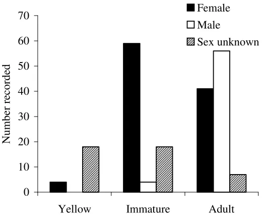
Figure 7. Size class distributions for the population of green python Morelia viridis at Iron Range, Australia. See text for details on size class limits.

Sexual dimorphism

Male and female green pythons are broadly similar in their body shapes. The mass of green pythons relative to their length was not significantly different between the sexes (slopes; t157 = 0.08, p = 0.936, intercepts; t157 = -0.05, p = 0.959, Figure 8a).

Nor did the tail lengths differ between the sexes at the same body length (restricted to individuals with complete tails, slope; t153 = -1.02, p = 0.309, intercept; t153 = 1.05, p =

0.297, Figure 8b). Partial tail loss occurred in only three individuals. There were however, significant differences between the sexes in head shape (both length and width). Females had both longer and wider heads compared with males of the same SVL, but male heads increased in both dimensions more quickly than those of

equivalent length females (length; slope; t107 = 2.41, p = 0.018, intercept; t107 = -2.43, p

= 0.017: width; slope; t107 = 2.28, p = 0.024, intercept; t107 = -2.28, p = 0.024, Figure 8c

(30)

[image:30.612.119.448.76.394.2]

Figure 8. Relationships between the snout-vent length of individual green pythons Morelia viridis at Iron Range and other morphometric variables measured; females – filled triangles and solid line; males – open nabla and broken line. All data has been transformed with natural logarithms. X – axis, snout-vent length.

I found no evidence of a difference in body condition between the sexes for either wet season where I sampled intensively (main effects; sex t150 = -0.2, p = 0.846, season

t150 = 0.3, p = 0.765, P for all interactions > 0.05 ).

I also found no significant differences between spur lengths of either sex (slope; t27 = 0.01, p= 0.995, intercept; t27 = 0.03, p = 0.973).

Sex ratio

Overall, I caught 60 males and 104 females where sex could be determined. The overall proportion of males in the population was 0.36, which was significantly different from parity ( 21= 11.95, p=<0.001). However when only adult individuals

(31)

On green pythons

two seasons when

2003-4). In the wet season of 2002

4 I caught 21 males and 22 females. In neither of these years did the adult sex ratio

differ significantly fr

Ontogenetic colour change

Individuals were categorised as yellow, green or changing (if they showed

(32)

[image:32.612.120.439.117.330.2]

(numbers on the x-axis represent the upper limit of each snout-vent length grouping).

Figure 10. Individual in the process of changing colour from yellow to green.

Discussion

This study is the first to detail the life history characteristics of green pythons in the wild, and presents rare information on a tropical, arboreal python. The four most important results were that; (1) green pythons have a strongly seasonal, but less than annual breeding cycle; (2) individuals are predicted to live for a considerable time (at least 15 years), with half the population consisting of adults; (3) there is a small degree of sexual dimorphism among juveniles but none discernible among adults; and (4) colour change in green pythons appears to be size mediated, and occurs within a very limited size range between 53 and 59 cm which corresponds to approximately one year of age.

Life history

(33)

On green pythons ₂₅

than the largest male (142 cm compared with 128 cm), suggesting that the asymptotic length A, may be slightly different between the sexes.

Males mature at smaller sizes than females (Shine & Slip 1990), and my data suggest that they reach maturity approximately 1.2 years earlier. This difference in maturity age of approximately one year is common in snakes (Parker & Plummer 1987). Based on a predicted hatching date in late November males mature in the middle of their third year, while females mature the following year. Maturity is reached at a similar length for both sexes of another Australian tropical python, Liasis fuscus, and for the more arid Astipides melanocephalus (Shine & Slip 1990). This predicted hatching date agrees with the three hatchings that I caught in early January. The predicted maximum age of approximately 19 years is near the upper limit of ages recorded for other snake species in the wild (Parker & Plummer 1987), however slightly less than the 20 years recorded from green pythons in captivity (Maxwell 2003). This value should be viewed with caution as confidence intervals were very wide for old individuals, and few individuals would reach this age.

Size class comparisons revealed that there were low numbers of juveniles in the population, and that immature individuals were predominantly female. The low number of juveniles detected is probably due to high juvenile mortality as most snake studies report high mortality within the first year of life (Parker & Plummer 1987). It may also be due to two types of sampling error. First, hatching and initial dispersal for green pythons may occur during periods when I was not in the field. This is unlikely as my data suggest most individuals hatch in late November near the beginning of my major research period. Second, hatching sites for green pythons have never been observed and it may be that neonates hatch and initially forage in areas where I did not search. However, I did catch three young individuals within a month of hatching. These three were found within five metres of each other. This suggests that I was searching in the appropriate habitat, and that neonates move very little during the first months of life. This agrees with my radio-tracking data (Chapter III) that showed average daily movements of 3 metres for the smallest individuals.

(34)

Interestingly, I found no evidence of sexual size dimorphism (SSD) in either weight or tail length for green pythons. Although females mature at slightly longer sizes (Shine & Slip 1990) and may grow to slightly longer maximum lengths, there was considerable overlap in body size between the sexes. I also found no difference in spur lengths between the sexes, refuting the findings of previously published studies (Barker & Barker 1994; Shine & Slip 1990). In contrast, I found sexual dimorphism in head characteristics at small body lengths, with females having larger heads than males (both length and width). As prey size in snakes is limited by the dimensions of an

individual’s gape (Arnold 1993), small differences in head shape between young males and females may result in dietary niche separation, possibly reducing intraspecific competition (Bolnick 2001). This may be important if individuals do not disperse rapidly from their hatching site and compete with siblings for food. As mortality is highest in the first year of life for most snake species (Parker & Plummer 1987), sexual differences may be less important and therefore lost as adults. In comparison, King et al. (1999) found varying levels of sexual dimorphism in a range of morphological traits for neonates and adults of four colubrid snake species. In general sexual dimorphism was either present in the same direction for neonates as adults, or occurred in adults but not neonates (King et al. 1999).

(35)

On green pythons ₂₇

Reproduction appears to be infrequent in the population as is typical for most Australasian python species (Madsen & Shine 1996a; Shine & Slip 1990). None of the adult females I captured, nor any of the 21 individuals radio-tracked for up to 18 months (Chapter III) showed any sign of reproductive activity. Further, mating, egg-laying and brooding in green pythons have never been observed in the wild. Female green pythons may delay reproduction until they have sufficient energy reserves, as has been shown in other snake species where not all adult-sized individuals breed in any year (Bertona & Chiaraviglio 2003; Madsen & Shine 1999; Reading 2004).

We can however deduce some details of the breeding cycle from my data, and from observations of the snakes in captivity. Extrapolation from the growth rates of individuals less than 45 cm suggests that hatching occurs in late November,

corresponding to the commencement of the wet season. I used only individuals within 15 cm of hatching as growth rates are highly variable in snakes (Madsen & Shine 2000), and individuals within this size range will have had less chance to diverge in their growth rates than larger individuals. Given that females are oviparous and in captivity brood their eggs for approximately 50 days (Maxwell 2003) my data suggests that laying occurs in early October. Hence it appears that green pythons in northern Australia have a strongly seasonal reproductive cycle with oviposition in the late dry season and hatching in the early wet season. Simulation of seasonality by lowering then raising temperature and humidity is also required to trigger egg laying in captive green pythons (Maxwell 2003).

The timing of emergence of neonate green pythons appears to coincide with the peak availability of their main food sources at Iron Range, Carlia longipes and diurnal invertebrates (Chapter IV). A seasonal reproductive pattern has also been shown in a related species, Liasis fuscus, where both oviposition and hatching occur at similar times to those suggested here for green pythons (Madsen & Shine 1996a). Following the predicted hatching date in late November there is increased activity in adult green pythons of both sexes until March, which I attribute to mate searching (Chapter III). From April until the beginning of the next breeding season in October individuals are relatively sedentary and inactive (Chapter III).

Ontogenetic colour change

(36)

morphs and the three individuals I observed changing were all within the maximum 3 cm recorded for yellow morphs. This suggests that OCC in green pythons is strongly size mediated. In captivity this change had been recorded to occur between six months (Switak 1975) and three years (Worrell 1951), however the age that OCC occurs in the wild appears to be more constrained. Based on the growth model (Figure 6) individuals change colour when they are approximately one year old. This change does not

coincide with sexual maturity, as the smallest recorded adult male and female were 84 and 99 cm respectively (Shine & Slip 1990). The ecologically convergent species C. caninus of South America shows similar OCC, with the colour change occurring in the same size range of 55 to 60 cm (Stafford & Henderson 1996). The underlying causes of colour change in C. caninus have never been studied, but may be similar to those of the green pythons given their strongly convergent ecological attributes.

Although colour change has long been of interest to scientists (Cott 1957; Poulton 1890), its evolutionary significance is still poorly understood (Booth 1990). The first step in understanding the significance of OCC in a species is to determine accurately the conditions under which it occurs. The function of colour can be separated into four distinct categories – intraspecific and interspecific communication, light-mediated functions (primarily thermoregulation) and physical pigment properties (Booth 1990). For green pythons the main function of colour appears to be in interspecific

communication – opportunities for intraspecific visual communication appear to be limited due to their solitary nature and nocturnal activity patterns. Colour mediated interspecific communication can involve crypsis, mimicry and aposematism (see review by Baylis (1979)) and is most often related to predation. Green coloration is common in arboreal snake species and has evolved as a form of crypsis against the foliage (Lillywhite & Henderson 1993), as concealment from both predators and prey. Although both red and yellow juvenile morphs exist in green pythons I will restrict this discussion to the change from yellow to green, as red morphs were not observed during my fieldwork, and have not been recorded from Australia.

(37)

On green pythons ₂₉

originated (Rawlings & Donnellan 2003). Such a species could explain the restricted size range over which the colour changed –yellow individuals larger than the model are rapidly selected against. Colour change from mimetic to cryptic as individuals outgrow the mimetic model has been shown for other snake species (Greene & McDiarmand 1981; Madsen 1987). Second, as many animals grow they move from one habitat to another, and if their background colour changes then they will also have to change colour if they are to remain cryptic. Habitat preferences do change with size in green pythons (Chapter III), with yellow individuals restricted to more open areas where light reached the ground, while green individuals were primarily found in closed canopy forests. A similar situation occurs in Corallus grenadensis where yellow individuals are found in sun-drenched habitats, while in ‘darker’ habitats only taupe or brown

individuals are more common (Henderson, 2002). Yellow individuals may be more cryptic to both predators and prey in open habitats than under a closed canopy rainforest. This appeared to be the case from my observations, but can only be accurately determined using spectroradiometry and the eye properties of predator and prey species (see Chapter V). With the timing of OCC in green pythons now

(38)

[image:38.612.60.762.155.509.2]

Table 1. The evolutionary significance of ontogenetic colour change. Table adapted from Booth (1990). Colour change

associated with;

Suggested reason; Adaptive value Possible in green pythons?

mimicry

small individuals mimic distasteful or dangerous species, and lose their mimicry when they outgrow the model, or when they reach a size where they are less vulnerable to predation

Yes

crypsis colour cryptic on small individuals, but not on large ones Yes

aposematism bright colour acts as a warning that they are distasteful or dangerous, toxicity changes with size

Unlikely – eaten by indigenous people in New Guinea, and not dangerous when small

thermoregulation colour affects absorption of solar radiation – less important as individuals grow

Unlikely – thermoregulation is less important for many tropical species (Shine & Madsen 1996) change in size and/or

vulnerability

deflection marks, intraspecific aggression,

variety of adaptive values related to intra and interspecific

communication Unlikely

mimicry no benefit of mimicry unless model occurs in new habitat Unlikely change in habitat

crypsis new habitat has different background, then individual need to

(39)

On green pythons ₃₁

thermoregulation, water balance, photoprotection,

different size individuals have different requirements Unlikely – thermoregulation not observed in either morph

change in reproductive status

immature individuals signal that they are not a threat, change to signal their availability to mate.

No – colour change does not occur at maturity (Shine & Slip 1990)

(40)

Chapter III

Age and sex related differences in the spatial ecology of a dichromatic

tropical python (

Morelia viridis)

(41)

On green pythons ₃₃

Abstract

(42)

Introduction

One of the most striking differences between temperate and tropical fauna is the difference in the number of arboreal species occurring in each zone. In the tropics more than three quarters of all vertebrate species are at least partially arboreal (Kays & Allison 2001). Within the arboreal vertebrate fauna of the tropics research is unevenly distributed across taxa, with mammals (especially primates) and birds receiving the most attention. There have been very few studies of arboreal reptiles and amphibians in tropical environments (Kays & Allison 2001), despite the tropics containing the

majority of species in these two taxa (Vitt 1987). Most major snake lineages include both tropical species and arboreal specialists (Lillywhite & Henderson 1993). The independent evolution of arboreality in snakes from separate lineages has been accompanied by striking convergence in morphology, ecology and behaviour

(Lillywhite & Henderson 1993), presumably reflecting similar ecological pressures. In Australia all snake families include species with arboreal and tropical representatives, with these traits most pronounced in the Australian pythons (Greer 1997). In general, arboreal species have attracted less scientific attention than their terrestrial counterparts, presumably due to logistic constraints (Bell et al. 1991). Radio-telemetry offers a solution to this problem, and can provide insights into otherwise cryptic, arboreal species (Fitzgerald et al. 2002; Webb & Shine 1997a).

In this study I used radio-telemetry to examine the sexual and age related differences in spatial ecology and movements of the green python (Morelia viridis: Pythonidae) - a rainforest species restricted to New Guinea and northern Cape York Peninsula, Australia (O'Shea 1996). M. viridis is a small ambush predator (maximum of 1.6 m) and the most arboreal species in the genus Morelia (Greer 1997). Morelia viridis shows complete ontogenetic colour change with juvenile individuals changing from either yellow or red to green adults, with the change for yellow individuals occurring between 55-60 cm (Chapter II). Morelia viridis shows one of the most striking examples of ontogenetic colour change, and determining whether or not differences exist in the ecology of the two colours morphs is an important step in understanding the evolutionary significance of this change. The underlying reasons for ontogenetic colour change are not yet well understood, yet this phenomenon occurs in a wide range of species (Booth 1990).

(43)

On green pythons ₃₅

spilota; (Heard et al. 2004; Pearson et al. 2005; Shine & Fitzgerald 1996; Slip & Shine 1988b), while preliminary studies have been undertaken on a second species (M. kinghorni; Fearn et al 2005, A. Freeman pers. comm.). Both species are primarily large and terrestrial (Greer 1997), with the studies done in temperate (M. spilota) or

subtropical environments (M. kinghorni). These studies can be used to contrast my results from a tropical arboreal species with those from closely related, yet ecologically dissimilar species.

Here I present data that reveal unexpected sexual and age-related differences in the home range and movement patterns of M. viridis that may be typical of tropical, arboreal snakes. This study is important because it highlights differences with closely related, yet more temperate and terrestrial taxa. It also provides important information on juvenile snake behaviour, which is generally lacking when compared to adult behaviour of the same species.

Methods

Study site

This study occurred in Iron Range National Park on Cape York Peninsula, in north-eastern Australia (12°45`S, 143°17`E, see Figure 3 in Chapter II). Within this park there is about 500km2 of lowland tropical rainforest in a complex mosaic with eucalypt woodland and heath (Neldner & Clarkson 1995). Mean annual rainfall for the park is 2123 mm (Bureau of Meteorology 1957-99 average) with most rain falling during a distinct ‘wet’ season from December to April.

Radio-tracking

Individual pythons were found by spotlighting, and surgically implanted with radio-transmitters (models SB-2 and BD-2G - Holohil Pty Ltd, Canada) by a veterinary surgeon (Peter Barrett – Marlin Coast Veterinary Clinic) following the procedure of Webb and Shine (1997b). Transmitters weighed 5 g (SB-2) or 1.85 g (BD-2G) for green and yellow individuals respectively, and were always <5% of body mass for any

individual (2.3 - 4.4% and 0.8 - 5.0 % of body mass for yellow and green individuals respectively). All individuals were released at their point of capture within 72 hours. I located individuals with an ICOM-R10 receiver and Yagi 3-stage antennae

(44)

they move from their day resting sight to their ambush site, and between 4-8am when they return to a resting posture (Chapter IV). Active individuals were never observed outside these times, and no individuals changed their resting site during the day, nor hunted at more than one location in a single night. Hence, consecutive fixes of an individual were always separated by a potential activity and location change. The order in which animals were tracked both within and among days was changed to avoid temporal autocorrelation in the data (Harris et al. 1990). Each location was marked with flagging tape and its position recorded with either a GPS (Garmin 12XL), or by using the distance and bearing from either previous locations or prominent landmarks. Due to their arboreal nature, individuals were often concealed from my view, either by foliage or because they were too high to be observed, when I estimated its location. If a new location for a concealed individual was within one metre of the previous location I considered that it had not moved. I report home range and movement results in two dimensions only, despite M. viridis being arboreal and operating in a three dimensional space. During radio-tracking I rarely recorded individuals close to the ground during the day, and often they were too high to observe and determine vertical position. Chapter 3 shows that individuals use all vegetation strata from the ground to the canopy, however this is not represented in the data. Similarly the movement distances were reported as if locations were on the same plane, rather than in three dimensional space. As I have no information on the relative heights at each location, true distances cannot be calculated. In this paper I used the two colour categories yellow and green to define different groups of M. viridis. Individuals change from yellow to green at approximately 55 centimetres SVL (Chapter II), however males do not mature until 84 centimetres, and females not until 99 centimetres (Shine & Slip 1990).

Data analysis

(45)

On green pythons ₃₇

polygons . All home range analysis was done using the RANGES 6 computer program (Kenward et al. 2003). The relationships between home range size, snout-vent length (SVL), month and sex were examined using a generalised linear modelling approach. In all cases residuals were examined to confirm that data were normally distributed, otherwise data were transformed to achieve normal distributions. As data from green males did not suggest a home range, I generated a sequential movement path. Home range overlap between pairs of green female M. viridis was determined using the 100% minimum convex polygons, while visual comparison between green male movement paths and green female home ranges was used to determine overlap between the sexes. Figures and movement paths were generated in ArcView GIS Version 3.1 with the Animal Movement Extension (Hooge et al. 1999).

I based the movement analysis on consecutive day fixes only, as longer intervals between fixes may underestimate daily movements. Consecutive fixes may also underestimate movement distances if individuals return to the same resting site after a period of movement. I observed green pythons re-using particular sites, however movements between these fixes were only in the vertical plane (descending to the ground and returning). Within this study, individuals never returned to a specific location after using a new site. As my data entailed repeated measures of individual snakes I avoided pseudo-replication by fitting generalised linear mixed models

incorporating the random factor “individual” in addition to the fixed variates and factors of interest. In all models both ‘season’ and ‘year’ were co-linear with ‘month’, therefore only ‘month’ was included in analyses.

I analysed movement in two ways. First, I analysed movement distances. Variables of interest in both analyses were SVL, the month and sex of the snake. All variables were removed sequentially from a fully factorial design to determine their significance. Movement distance was analysed with a linear mixed model, testing for the effects of SVL, month and sex. As the residuals were not normally distributed, distances were transformed using natural logarithms to obtain a better fit to the data.

(46)

[image:46.612.60.503.254.735.2]

Between November 2002 and April 2004 I recorded 2178 fixes from 27 pythons (9 green and 1 yellow male, 12 green and 5 yellow females, Table 2). This period encompassed two wet seasons and the intervening dry season. Individuals were tracked for a mean of 143 days (range 15-449), with a mean of 80 fixes (range 9-251) per individual. Three individuals were monitored for the whole study, while all others were monitored for at least a single wet season. I did not detect any female reproductive activity (egg formation or laying) during the study.

Table 2. Individual green pythons Morelia viridis radio-tracked during this project

Snake ID Sex Colour SVL†

(cm)

Mass (grams)

Capture date

Tracking duration (days)

Number of fixes

Gladys Sym Choon F Yellow 51.5 46 2-Jan-03 27‡ ₁₅

Judith F Yellow 51.5 51.5 21-Nov-02 6‡ ₁₁

Hepzibar F Yellow 51.7 42.5 9-Jan-03 86 62

Xanthippe F Yellow 52.4 52 21-Dec-03 58 67

Elephant F Yellow 56.0 68 2-Dec-02 65 83

Yellow females – means ± s.e. 53.1 ± 0.9 52.3 ± 4.4 69.7 ± 8.4 70.7 ± 6.3

Thor F Green 62.7 81 9-Jan-03 86 62

Vera Lynn F Green 70.0 99 3-Jan-03 132 51

Limburger F Green 81.6 177 31-Jan-04 10§ ₉

Utopia F Green 82.0 143 15-Oct-03 195 144

Chesterfield F Green 92.2 254 19-Jan-03 188 78

Ra F Green 96.0 284 16-Jan-03 132 60

Pont L'Eveque F Green 96.3 238 31-Jan-04 56 55

Pleasure Machine F Green 102.0 281 2-Dec-02 180 94

Zarniwoop F Green 102.3 258 19-Jan-03 119 57

AntiChrist F Green 111.5 472 9-Jan-03 444 130

Drench F Green 115.0 515 7-Jan-03 142 83

Tilsit F Green 142.0 617 7-Jan-04 89 65

Green females – means ± s.e. 96.1 ± 6.2 284.9 ± 48.5 160.3 ± 31.3 79.9 ± 9.4

Cookie Monster M Yellow 55.8 67 21-Dec-03 60 54

Yellow males - mean 55.8 67 60 54

Manhattan M Green 72.5 115 9-Jan-03 198 87

Ilchester M Green 87.8 152 31-Jan-04 61 57

Quinquervina M Green 88.0 189 28-Oct-03 154 133

Brian M Green 89.4 229 9-Jan-03 445 251

Faislabad M Green 91.4 237 13-Jan-03 79 44

(47)

On green pythons ₃₉

Wonko the Sane M Green 98.5 301 9-Jan-03 129 57

Kubla Khan M Green 103.0 421 16-Jan-03 438 194

Rasputin M Green 105.8 445 21-Dec-03 108 102

Green males – means ± s.e. 92.4 ± 3.3 261.9 ± 37.5 188.7 ± 49.7 110.9 ± 23.4

†_{SVL, snout-vent length.}

‡_{These transmitter failed earlier than expected.} §_{This individual was killed by a predator.}

Home range

(48)

[image:48.612.80.478.58.341.2]

Figure 11. Incremental area plots for Morelia viridis home ranges: (a) green males, (b) green females, and (c) yellow individuals.

These analyses exclude individuals with less than 20 locations. Note the three graphs have different scales for the x-axes, due to differences in transmitter life between groups. The solid line represents the mean home range area as a percentage of final home range for all individuals, while the vertical lines are the 95% confidence intervals associated with the mean at each fix.

(49)

On green pythons ₄₁

[image:49.612.133.523.155.510.2]

period 3.3 ± 0.5 (mean ± SE, range 2 – 4) radio-tracked green males passed through a green females’ home range. I caught other green males within the home range of green females and therefore the number of males passing through a female’s home range reported here is also an underestimate.

Figure 12. Home range areas of four radio-tracked individuals.

Two were green females a) Tilsit, and b) Drench (enclosed polygon). Also shown are the movement paths of three green males (thin lines), activity areas of two yellow individuals (shaded polygons) and other individuals (dots) found in their home ranges during the radio-tracking period. Movement paths of two green males c) Kubla Khan, and d) Ilchester.

Movement

Movement distance. The distance travelled between fixes by an individual was

(50)

[image:50.612.113.444.142.300.2]

however this was not always the case for different month/sex combinations.

Table 3. Results for the generalized linear mixed model testing movement distances of individual Morelia viridis. Terms were added sequentially to the fixed model

Effect X2 DF P

SVL 14.28 1 <0.001

Month 12.85 9 0.169

Sex 0.40 1 0.525

SVL.Month 6.01 9 0.739

SVL.Sex 0.09 1 0.766

Month.Sex 30.91 8 <0.001

SVL.Month.Sex 29.95 7 <0.001

During the wet season larger females moved further in February than in other months (Figure 13a), while larger males moved further in January and March (Figure 13b). During the dry season movement distances varied more between individuals than during the wet (compare the error bars in Figure 13c and 13d with those in 13a and 13b

respectively). Distances moved for all individuals in most months varied from 3 – 23 metres per move (values back transformed from predicted means). In January, February and March however the average maximum distance moved increased to approximately 50 metres. The data were highly skewed, with only eight of 1057 consecutive

(51)

On green pythons ₄₃

analysed statistically this trend was more obvious in larger individuals, and seemed to occur more during the wet than the dry season.

Figure 13. Predictions of the natural logarithm of distance moved for individual snakes at various times of the year.

[image:51.612.141.529.115.371.2]

Predictions reflect the significant interaction between x, y and z. (a) females, and (b) males during the wet season. The three lines represent January , February and March ; (c) females, and (d) males during the dry season. The three lines represent the months of May , September , and November . Standard errors are shown.

Table 4. Selected daily movement sequences for four Morelia viridis at Iron Range National Park.

Individual Movement distances (metres)

Antichrist (F) 0, 0, 70, 56, 16, 3, 5 and 0, 0, 60, 21, 0, 0 Brian (M) 0, 0, 94, 21, 42, 0, 0 and 0, 0, 42, 28, 85, 0, 0 Kubla Khan (M) 0, 0, 8, 142, 0, 0 and 0, 11, 39, 28, 28, 3, 5 Pont L’Eveque (F) 0, 32, 39, 2, 0, 0 and 0, 7, 2, 9, 65, 25, 3, 0

(52)

both the size of the individual (X21 = 0.49, P = 0.520) and the month (X28 = 12.68, P =

0.123)

Discussion

My study is one of the few to provide home range data for a tropical, arboreal snake. The data revealed two notable aspects of the ecology of M. viridis that may have broader implications for snakes in general. First the two sexes of M. viridis adopt different movement strategies, with green females having a home range and males ‘roaming’ across the landscape. This applied to all adult males, rather than a small subset of individuals. This sexually divergent strategy has not been reported previously for either of the other intensively studied Morelia species (Fearn et al. 2005; Slip & Shine 1988b), and to my knowledge has not been conclusively shown in any other snake species since the review of Parker and Plummer (1987). Second my data contributed detailed information on the movement patterns of juvenile snakes, which are unknown for most species. Yellow M. viridis moved as often as green individuals, and for comparable distances most of the year, despite being considerably smaller. They also lacked a home range, presumably as they were dispersing from their hatching site.

Home range

I used the criteria that defined a home range to exist when an incremental area plot plateaus at greater than 80% of the range area asymptote (Rose 1982; Stone & Baird 2002). I found that green females did have a home range, while both green males and yellow individuals did not. The average green female home range size of 6.21 ha is well within the range of home range sizes reported for other snake species (Macartney et al. 1988). The home range for female M. viridis is considerably smaller than the home range reported from the closely related M. spilota where females had a mean home range of between 11 and 37 hectares (Shine & Fitzgerald 1996; Slip & Shine 1988b). This difference is not unexpected as M. spilota are typically much larger as adults (Shine & Slip 1990) and use a correspondingly larger area (Jetz et al. 2004).

On green pythons : the ecology and conservation of Morelia viridis

Declaration

Abstract

Acknowledgements

Contents

Figures

Tables

General Introduction

Chapter II

Life history traits and ontogenetic colour change in an arboreal

tropical python,

Morelia viridis

0

5

10

15

20

25

30

35

Ju

ly

A

ug

us

t

S

ep

te

m

be

r

O

ct

ob

er

N

ov

em

be

r

D

ec

em

be

r

Ja

nu

ar

y

Fe

br

ua

ry

M

ar

ch

A

pr

il

M

ay

Ju

ne

Te

m

pe

ra

tu

re

(C

)

0

50

100

150

200

250

300

350