Nernst branes from special geometry

LTH-1033

Nernst branes from special geometry

P. Dempster1,2_{, D. Errington}1 _{and T. Mohaupt}1 1_{Department of Mathematical Sciences}

University of Liverpool Peach Street Liverpool L69 7ZL, UK

[email protected], [email protected], [email protected] 2_{School of Physics & Astronomy and Center for Theoretical Physics}

Seoul National University Seoul 151-747, KOREA

January 30, 2015. Revised: February 27, 2015.

Abstract

We construct new black brane solutions inU(1) gaugedN = 2 supergravity with a general cubic prepotential, which have entropy density s ∼T1/3 as T →0 and thus satisfy the Nernst Law. By using the real formulation of special geometry, we are able to obtain analytical solutions in closed form as functions of two parameters, the temperatureT and the chemical potentialµ. Our solutions interpolate between hyperscaling violating Lifshitz geometries with (z, θ) = (0,2) at the horizon and (z, θ) = (1,−1) at infinity. In the zero temperature limit, where the entropy density goes to zero, we recover the extremal Nernst branes of Barischet al, and the parameters of the near horizon geometry change to (z, θ) = (3,1).

Contents

1 Introduction 2

2 _N = 2 gauged supergravity and the real formulation of special geometry 7

2.1 Lagrangian of_N = 2U(1) gauged supergravity . . . 7

2.2 Reduction to three dimensions . . . 9

2.3 Purely imaginary field configurations . . . 11

3 Non-extremal black branes 12 3.1 Einstein equations . . . 13

3.2 Scalar equations of motion . . . 13

3.3 The Nernst brane solution . . . 17

3.4 Properties of the Nernst brane solution . . . 19

4 A magnetic black brane 23

5 Discussion and conclusions 24

A Scalar potential in the real formulation of special geometry 28

B Adapting the real formulation of special geometry to dimensional reduction 31

1

Introduction

One of the most celebrated successes of string theory is the AdS/CFT correspondence [1]. This generates a powerful duality between asymptotically AdS gravitational theories and conformal field theories on the AdS boundary, which is the simplest and best-studied example of the more general notion of a ‘gauge-gravity duality’. As a strong-weak coupling duality, the cor-respondence allows for the translation of non-perturbative field theory calculations into more tractable, perturbative calculations in gravity and vice-versa. This has enabled the exploration of previously inaccessible regimes of theoretical physics. Indeed, there are many examples of strongly coupled systems in condensed matter physics and it is hoped that gauge-gravity dual-ity may allow for a better understanding of these. Significant progress has already been made in this direction, leading to the development of the AdS/CMT correspondence (see [2, 3] and references therein). Further recent progress has been to extend the correspondence to space-times which are not asymptotically-AdS but rather exhibit hyperscaling violating and Lifshitz (hvLif) behaviour [4, 5], thus extending the dictionary between gravity and condensed matter systems living on the boundary.

field theory with the same thermodynamic properties (temperature, entropy, chemical potential, etc.) as the bulk spacetime [6, 7].

A natural starting point for the correspondence is to look at charged (Reissner-Nordstr¨om or ‘RN’) extremal black holes and black branes in AdS [8]. However, like their asymptotically flat ‘cousins’ they have a large non-zero entropy at zero temperature, thus violating the Third Law of Thermodynamics, which states in its strictest version that the entropy of a system should vanish in the zero temperature limit [9]. While a non-vanishing entropy for certain classes of extremal black holes is consistent with microstate counting for the corresponding D-brane configuration in string theory [10, 11], this still begs the question of whether one can find other gravitational systems which have a zero entropy or entropy density at zero temperature. Apart from being an interesting question about gravity, such systems are relevant for possible dualities between gravity and condensed matter systems.

We remark that although ‘Nernst Law’ is in the following used synonymously with ‘Third Law of Thermodynamics’, Nernst’s original formulation only requires that the difference in entropy between two equilibrium states related through a change in external parameters goes to zero at zero temperature. This formulation is equivalent to the ‘process version’ of the Third Law, which states that zero temperature cannot be reached by any physical process in a finite number of steps. A process version of the third law of black hole mechanics was already established in [12]. However, the Nernst version or, equivalently, the process version of the Third Law does not imply by itself the slightly stronger version of the Third Law, due to Planck, which states that the entropy itself goes to zero at zero temperature. This stricter version corresponds to systems with a unique ground state, and thus is the generic situation in condensed matter, although there is an extended debate about possible exceptions in specific systems, see for example [2, 3, 13, 14].

In the following we will be concerned with the explicit construction of families of gravita-tional solutions which have zero entropy (or entropy density) in the extremal limit. Following conventions in the literature, we will refer to the Third Law in its stricter, Planckian, version as the Nernst Law.

field theory [2, 19]. A first step in addressing this issue is to find non-extremal solutions, which can then be studied in the near extremal limit. In this context it is clearly desirable to have completely explicit, analytical solutions. However most results in the literature have to rely on a mixture of analytical and numerical methods. Of course tidal forces may still get very large at the horizon when one approaches the extremal limit [20], but analytical solutions will enable one to identify the region in parameter space where the solution can be trusted and possibly be mapped to condensed matter systems.

The second step in controlling the near horizon low temperature behaviour is to embed the theory under consideration into a UV-complete theory, for which string theory and its non-perturbative extension M-theory are arguably the best candidates. In the low-energy limit the relevant stringy gravitational backgrounds can be described in terms of supergravity. We will be working in a set-up which can be described by N = 2 U(1) gauged supergravity with an arbitrary number of vector multiplets. Theories with N = 2 supersymmetry are natural generalisations of the Einstein-Maxwell-Scalar theories underlying dilatonic black hole and black brane solutions which have been studied extensively as potential duals of strongly coupled electron systems [2, 3]. They have the advantage that one can often find exact, analytical answers, despite the fact that the couplings are not fixed by the matter content (as is the case for N ≥4 supersymmetry), but depend on arbitrary functions of the scalar fields, which are subject to quantum and stringy corrections. While we do not discuss the string theory or M-theory embedding explicitly, note that such theories arise through heterotic flux compactifications on

K3×T2and type-II flux compactifications on Calabi-Yau three-folds. We will not need to choose a specific model, and only assume that the vector multiplet couplings take the most general form that arises when working to leading order in the Regge parameter α0_{, and within the validity}

of string perturbation theory. In other words, we only assume that the prepotential, which encodes the vector multiplet couplings, is of the so-called very special type reviewed below. By working in a gauged supergravity theory obtainable by flux compactification from string theory we will have the option to further address the issues related to singularities in the extremal limit at a later stage. For BPS black holes with vanishing entropy it is known that the inclusion of stringy higher curvature corrections in supergravity [21,22] leads to regular solutions with finite entropy [23], and the entropy function formalism demonstrates that this mechanism is robust and does not depend on supersymmetry and details of the higher curvature corrections [24]. We refer to [2, 3, 14] for a further discussion of the possible implications of quantum and string corrections to the zero temperature behaviour and the ‘fate’ of the Nernst Law.

proven elusive, and the only known examples [25] have been constructed by deforming the metric of the corresponding five-dimensional extremal solution [26] and imposing suitable consistency conditions. In this paper we are able to provide a systematic construction of non-extremal Nernst branes by directly solving the second-order equations of motion. Moreover, our results will not only apply to a particular model, but to all models where the prepotential is of the very special type. This gain in generality and systematics should help to expand the AdS/CMT dictionary considerably in the future.

We now present a brief overview of the results in this paper. We start with a theory ofn

N = 2 vector multiplets coupled toU(1) gauged supergravity, with prepotential

F(X) = f(X

1_{, . . . , X}n₎

X0 ,

wherefis homogeneous of degree three. Iff is a homogeneouspolynomialof degree three (which is not required for our methods to apply), then the corresponding theory can be obtained by dimensional reduction from five dimensions. Moreover, such prepotentials capture perturbative string effects to leading order inα0if the model can be embedded into heterotic or type-II string theory. In this case the supergravity lift to five dimensions becomes a lift from type-II string theory to M-theory.

Within these models we restrict ourselves to static black brane solutions. Apart from this we will impose that the scalar fields take purely imaginary values, as for such ‘axion-free’ field configurations there is a systematic simplification of the equations of motion. Since we impose stationarity in four dimensions, we can perform a time-like dimensional reduction to obtain an effective three-dimensional Euclidean theory. The degrees of freedom in three dimensions can then be repackaged using the real formulation of special geometry developed in [27], which has been used to construct solutions to both gauged [28–30] and ungauged [31] theories of supergravity coupled to vector multiplets.

Since our ability to obtain explicit non-extremal solutions depends on using a specific for-malism, let us briefly summarize the underlying principles without going into technical details. • Instead of using the physical four-dimensional scalar fields zA_{,A= 1, . . . , n, we work on}

the ‘big moduli space’ parametrized by scalar fields XI_{, I = 0, . . . , n. The additional}

(complex) degree of freedom is compensated for by a localC∗ _{gauge symmetry. Working}

on the big moduli space has the advantage that the number of scalar fields and gauge fields matches.

• We use the real formulation of special K¨ahler geometry, which replaces the complex scalars

XI by real scalarsqa,a= 0, . . . ,2n+ 1 and which replaces the holomorphic prepotential

• Upon dimensional reduction, the Kaluza-Klein scalarφ is absorbed into the real scalars

qa, which results in the ‘radial’ direction of the big moduli space becoming a physical (rather than gauge) degree of freedom.

We postpone fixing the remaining U(1) ⊂ C∗ _{gauge symmetry to preserve}

electric-magnetic duality. The resulting three-dimensional theory depends on 4n+ 5 real scalars

qa_,qˆa_,φ˜_{, subject to one local gauge symmetry, where ˆq}a _{are dual to the four-dimensional}

gauge fields and ˜φ is dual to the Kaluza-Klein vector. While qa_,qˆa _{are vectors under}

electric-magnetic duality, ˜φis a scalar.

• We impose an ansatz which corresponds, from the four-dimensional point of view, to a static solution with purely imaginary scalar fields. This determines ˜φand half of the fields

qa,qˆain terms of the remaining fields, and also fixes the residualU(1) gauge symmetry. By abuse of notation, we denote the remaining independent fields byqa,qˆa (with a restricted range ofa, depending on the precise version of the ansatz).

• When we now proceed to solve the time-reduced three-dimensional equations of motion, their particular structure allows us to obtain solutions in closed form.

We remark that while some of the above ingredients are well known to people working on _N = 2 supergravity, it is critical that these elements are put together into a systematic structure. The key element that we use and preserve is electric-magnetic duality, which acts on the fields by symplectic transformations.1 _{Our choice of variables, which all transform as} symplectic tensors, leads to the simplifications and systematics that we exploit. We observe that this works despite the fact that the electric-magnetic duality group is broken to a discrete subgroup thereof by the presence of gauging (a scalar potential), and despite the fact that our ansatz restricts us from the full symplectic group to a subgroup.

Solving the three-dimensional equations of motion directly results in an instanton solution depending on a number of integration constants, which are a priori undetermined. However, in order that this solution lifts to aregular black brane in four dimensions we have to impose suitable regularity conditions. In particular, we require that the four-dimensional solution has a finite entropy density, which happens to simultaneously ensure that the scalar fields take finite values on the horizon. For a given set of charges and fluxes, we are then left with a two-parameter family of black brane solutions parametrised by a temperatureT and chemical potential µ, which can both be freely varied. In the limit of zero temperature, we recover the extremal Nernst branes of [19]. Therefore we interpret our solutions as non-extremal (or ‘hot’) Nernst branes. Indeed, it turns out that the entropy density goes to zero as T _→ 0 for fixed charges/fluxes, in agreement with the Nernst Law. Our solutions interpolate between hyperscaling violating Lifshitz geometries with (z, θ) = (0,2) at the horizon and (z, θ) = (1,₋1)

at infinity, wherez is the dynamical critical exponent and whereθis the hyperscaling violating exponent. In the zero temperature limit the near horizon geometry changes to (z, θ) = (3,1).

This paper is organised as follows. In Section 2 we review the real formulation of special geometry as applied to N = 2 U(1) gauged supergravity with both electric and magnetic fluxes, relegating the more technical details to the appendices. We then reduce this theory over a time-like direction and determine the equations of motion of the three-dimensional theory for general static field configurations, before concentrating on the case of purely imaginary field configurations. In Section 3 we solve the aforementioned equations of motion for the case where we have a single electric charge and some number of electric fluxes. Having found a solution to the three-dimensional equations of motion we then lift it back to a four-dimensional solution and determine the conditions imposed on the various integration constants by regularity, before carrying out an analysis of the properties of the solution. In Section 4 we apply our method to the case where we instead switch on a single magnetic charge and a single magnetic flux, whilst keeping (n₋1) of the electric fluxes. Section 5 contains our conclusions. We also include a brief initial discussion of our results in the context of holography.

2

_N

= 2

gauged supergravity and the real formulation of

special geometry

2.1

Lagrangian of

_N

= 2

U

(1)

gauged supergravity

We begin with the well-known bosonic Lagrangian of N = 2 Fayet-IliopoulosU(1)⊂SU(2)R

gauged supergravity coupled tonvector multiplets. Our conventions follow those of [27, 29]2

e−₄1_L4=− 1

2Y R(4)−gIJ∂µˆX

I_∂µˆ_X¯J₊1

4IIJF

I

ˆ

µνˆF

J|µˆˆν₊1

4RIJF

I

ˆ

µνˆF˜

J|µˆˆν

−V X,X¯

, (2.1)

where ˆµ,νˆ = 0, . . . ,3 are four-dimensional spacetime indices, and I, J = 0, . . . , n label the four-dimensional gauge fields: n from the vector multiplets and one, the graviphoton, from the gravity multiplet. For later convenience we use a formulation of the theory which contains

n+ 1 complex scalar fieldsXI _{which are subject to local dilatations andU(1) transformations.}

The n physical scalars remaining after gauge fixing can be parametrised as zA _{= X}A_/X0_, where A = 1, . . . , n. While the physical scalars zA _{parametrise a projective special K¨ahler}

(PSK) manifold, the XI _{parametrise a conic affine special K¨ahler (CASK) manifold, which is}

a complex cone over the PSK manifold. Conversely, the PSK manifold can be obtained as the K¨ahler quotient of the CASK manifold with respect to theC∗_{-action generated by dilatations}

andU(1) transformations. In physical terms this quotient amounts to gauge fixing the localC∗

determined by the holomorphic prepotential F(XI), which is homogeneous of degree 2. Prior to gauge fixing dilatations, the space-time Ricci scalar, R4, is multiplied by the conformal compensator

Y =−i(XIF¯I −FIX¯I),

where derivatives of the prepotential are denotedFI = _∂X∂FI, etc. The tensor

gIJ =−

∂2

∂XI_∂X¯J logY,

is the horizontal lift of the physical (PSK) scalar metric to the CASK manifold. It has a two-dimensional kernel which reflects the fact that the XI only representn complex physical degrees of freedom. The vector couplings are given by

NIJ =RIJ+iIIJ = ¯FIJ+i

NIKXKNJ LXL

−XM_N M NXN

,

whereNIJ = 2ImFIJ.

We now turn to theC∗ _{gauge fixing. Dilatations are fixed by imposing the D-gauge}

−i XIF¯I−FIX¯I

=κ−2, (2.2)

which in particular brings the Einstein-Hilbert term in (2.1) to the standard form ₋₂1_κ2R4.

LikewiseU(1) transformations can be fixed by imposing any condition transverse to theU(1) action, such as Im X0 = 0. However, as discussed in more detail in [27, 31], it is often advantageous to postponeU(1) gauge fixing until reducing the theory and starting to solve the resulting equations of motion. In particular, upon imposing the D-gauge (2.2) one has

gIJ∂µˆXI∂µˆX¯J= ¯gAB∂ˆµzA∂µˆz¯B,

where ¯gAB is the positive definite (PSK) metric of the physical scalars zA. Working with the

scalarsXI _{has the advantage that we retain covariance under symplectic transformations, and}

will result in a more convenient form of the equations of motion after reduction. Note that while the D-gauge removes one real degree of freedom from the XI_{, the second unphysical}

degree of freedom is taken care of by the remaining local U(1) symmetry, see [27] for details. Geometrically, imposing the D-gauge while keeping the local U(1) symmetry corresponds to working on aU(1) principal bundle over the PSK manifold.

The four-dimensional Lagrangian (2.1) also includes a scalar potential V(X,X¯), which as in [19] is given as

with a superpotential of the form

W = 2 gIFI−gIXI

, (2.4)

wheregI_{, g}

I parametrize theU(1) gauging. Since superpotentials of the form (2.4) arise in flux

compactifications, we refer to them as magnetic and electric fluxes, respectively. Note that we have included an explicit factor ofκ2 in (2.3) using dimensional analysis. We will use this later to rewrite the potential in terms of real variables. For reference, we note that the XI have mass dimension −1 while the flux parameters have dimension −2, so that W has dimension −3. SinceNIJ and, hence, its inverseNIJ are homogeneous of degree 0, they have dimension

0, andV has dimension ₋4, as required. We also remark that for later convenience we have re-scaled the flux parameters by a factor of 2 relative to [19]. Moreover, we have not factorized the flux parameters into a dimensionful coupling and dimensionless parameters, but kept them dimensionful.

2.2

Reduction to three dimensions

Imposing that the background is stationary, so that all of the fields are independent of time, we can reduce the four-dimensional action (2.1) over a time-like direction in order to obtain an effective three-dimensional Euclidean action. We decompose the four-dimensional metric as

ds2₄=₋eφ(dt+Vµdxµ)2+e−φds23, (2.5)

whereφandVµare the Kaluza-Klein scalar and vector respectively, and we have left the

three-dimensional part of the metric undetermined for now. Following the procedure for time-like dimensional reduction outlined in [27], and noting that the scalar potential remains unchanged throughout the reduction process, one obtains the three-dimensional Lagrangian [29]

e−₃1_L3 = − 1

2R(3)−H˜ab ∂µq

a_∂µ_qb

−∂µqˆa∂µqˆb

+ 1 2HV

−_H12(q

a_Ω

ab∂µqb)2+

2

H2(q

a_Ω

ab∂µqˆb)2

−_4H12(∂µφ˜+ 2ˆq

a_Ω

ab∂µqˆb)2. (2.6)

We have written all of the three-dimensional degrees of freedom using the conventions of the real formulation of special geometry developed in [27], and afterwards setκ= 1 for the remainder of the paper. While we give a brief summary here, more details can be found in Appendix B. The three-dimensional action contains 4n+ 5 scalar fields (qa_,qˆa_,φ˜_{) which are subject to one}

local U(1) symmetry and hence has 4n+ 4 independent scalar degrees of freedom. While the

vector. The constant tensor

Ωab=

0 1

−1 0

!

is the symplectic form of the CASK manifold expressed in real variablesqa. The tensor ˜Habis

given by

˜

Hab=

∂2_H˜

∂qa_∂qb , H˜ =−

1

2log(−2H),

where the Hesse potentialH is related to the prepotentialF by the Legendre transformation given in (A.1).

As shown in the appendices, the scalar potentialV is given in terms of the real coordinates as

1

HV(q) =−2g

a_gb

˜

Hab−4qaqb−2

(Ωq)a(Ωq)b

H2

, (2.7)

where the dual scalarsqa are defined byqa =−H˜abqb.

Substituting this expression into (2.6) the three-dimensional Lagrangian becomes

e−₃1_L3 = − 1

2R(3)−H˜ab ∂µq

a_∂µ_qb

−∂µqˆa∂µqˆb+gagb

−_H12(q

a_Ω

ab∂µqb)2+

2

H2(q

a_Ω

ab∂µqˆb)2

+4(gaqa)2+

2

H2(q

a_Ω

abgb)2−

1

4H2(∂µφ˜+ 2ˆq

a_Ω

ab∂µqˆb)2. (2.8)

In the following we will restrict ourselves to static solutions, i.e. set Vµ = 0 in (2.5), for

which the final term in (2.8) vanishes [27]. The equations of motion for ˆqa are then given by

∇µ

˜

Hab∂µqˆb

+ 2∇µ ₁

H2q

b

Ωba(qcΩcd∂µqˆd)

= 0, (2.9)

whilst those forqa _read

∇µ

˜

Hab∂µqb

−1₂∂aH˜bc ∂µqb∂µqc−∂µqˆb∂µqˆc+gbgc

−1₂∂a ₁

H2

(qbΩbc∂µqc)2+∇µ ₁

H2q

b

Ωba(qcΩcd∂µqd)

−_H12Ωab∂µq

b

(qcΩcd∂µqd)

+∂a ₁

H2

(qcΩcd∂µqˆd)2+

2

H2Ωab∂µqˆ

b_(qc_Ω cd∂µqˆd)

+ 4 ˜Habgb(gcqc) +∂a ₁

H2

(qbΩbcgc)2+

2

H2Ωabg

b_(qc_Ω

cdgd) = 0. (2.10)

Finally, the three-dimensional Einstein equations are

−1₂R(3)µν−H˜ab ∂µqa∂νqb−∂µqˆa∂νqˆb

−_H12(q

a_Ω

ab∂µqb)(qcΩcd∂νqd)

+ 2

H2(q

a_Ω

ab∂µqˆb)(qcΩcd∂νqˆd) +gµν

−H˜abgagb+ 4(gaqa)2+

2

H2(g

a_Ω abqb)2

2.3

Purely imaginary field configurations

We concentrate in this paper on purely imaginary (PI) field configurations, which we define to be those for which the complex scalars3 _zA_=YA_/Y0 _{are purely imaginary [31]. Moreover, we} restrict ourselves to a class of prepotentials of the form

F(Y) =f(Y

1_{, . . . , Y}n₎

Y0 , (2.12)

where the function f is homogeneous of degree three and real-valued when evaluated on real fields. For the case of ungauged_N = 2 supergravity, such models were considered in [31]. Note that those models withf a cubic polynomial are precisely the ‘very special’ prepotentials for which the solutions can be uplifted to five dimensions. Since we choose to fix theU(1) gauge by taking ImY0= 0, this is equivalent to settingxA= ReYAto zero. Models obtainable from five dimensions are invariant under constant shiftsxA _→xA+CA, and, hence, PI configurations will be referred to as ‘axion-free’.

For the class of models (2.12) the scalar fieldsqa _{take the form [31]}

(qa)_|PI= (x0,0, . . . ,0; 0, y1, . . . , yn),

and hence we see thatqaΩab∂µqb= 0. Following [31] we extend the PI condition to the scalars

ˆ

qa by imposing

(∂µqˆa)|PI=

1 2(∂µζ

0_{,0, . . . ,0; 0, ∂}

µζ˜1, . . . , ∂µζ˜n),

which sets alsoqaΩab∂µqˆb = 0. The quantities∂µζI and∂µζ˜I encode the four-dimensional field

strengths, see (B.5).

In the same way, we extend the PI condition to the fluxesga _{by imposing}

(ga)_|PI= (g0,0, . . . ,0; 0, g1, . . . , gn),

which setsqa_Ω

abgb= 0.

We then find that the equations of motion (2.9)–(2.10) and the three-dimensional Einstein equations (2.11) simplify to

∇µ

˜

Hab∂µqˆb

= 0, (2.13)

∇µ

˜

Hab∂µqb

−1₂∂aH˜bc ∂µqb∂µqc−∂µqˆb∂µqˆc+gbgc

+ 4 ˜Habgb(gcqc) = 0, (2.14)

and

−1₂R(3)µν−H˜ab ∂µqa∂νqb−∂µqˆa∂νqˆb+gµν

−H˜abgagb+ 4(gaqa)2

= 0. (2.15)

It turns out to be useful to write the equations of motion in terms of the dual variables qa

and ˆqa defined in Appendix B. In terms of these, the equations (2.13)–(2.15) become

∇2_qˆ

a= 0, (2.16)

∇2qa+

1 2∂aH˜

bc_(∂

µqb∂µqc−∂µqˆb∂µqˆc)−

1 2∂aH˜bcg

b_gc_{+ 4 ˜H}

abgb(gcqc) = 0, (2.17)

and

−1₂R(3)µν−H˜ab(∂µqa∂νqb−∂µqˆa∂νqˆb) +gµν

−H˜abgagb+ 4(gaqa)2

= 0. (2.18)

In the next section we will look for solutions of (2.16)–(2.18) which can be lifted to regular non-extremal black branes in four dimensions.

3

Non-extremal black branes

Our aim in this section is to construct a family of non-extremal black branes in the _N = 2 gauged supergravity theory (2.1) with prepotential (2.12). Restricting our attention to the PI configurations described in Section 2.3, it can be shown that the Hesse potential takes the form [31]

H =−1₄(−q0f(q1, . . . , qn))

−1

2_{. (3.1)}

For general functionsf, the form of the metric ˜Hab is fairly complicated [31]. However, since the fieldq0decouples from the rest, we can compute

˜

H00= 1 4q2

0

, q0=₋ 1 4q0

,

and this will be sufficient to find solutions valid for any choice off. We remark here upon a slight abuse of notation which we will make throughout the remainder of this paper. Specifically, we denote by qA with A = 1, . . . , n those scalar fields which are actually the (A+n+ 1)’th

components of the vector (qa). The same is true of the components ˜HAB of the metric, which

should properly be the (A+n+ 1, B+n+ 1) components of ˜Hab. This notation is convenient

since (q0, qA) are the remaining non-trivialqa-fields within our ansatz.

For simplicity we will concentrate on solutions which are supported by a single electric charge Q0 and electric fluxes g1, . . . , gn in this section. However, as we will see in Section 4,

3.1

Einstein equations

We make a brane-like ansatz for the three-dimensional metric:

ds2₃=e4ψdτ2+e2ψ(dx2+dy2), (3.2)

where ψ = ψ(τ) is some function to be determined. This form of the metric can always be obtained from the more commonly used form ds2₃ = dr2+e2ψ_(dx2_+dy2_{) by a suitable} redefinitionr_→τ. We also impose that all fields qa and ˆqa depend only onτ. The coordinate

τ has been chosen such that it is an affine parameter for geodesic curves on the scalar target space parametrized byqa _{and ˆq}a_{. Equivalently, theτ-dependent part of the three-dimensional}

Laplace operator is given by ∂2

∂τ2.

The non-zero components of the Ricci tensor are given by

Rτ τ = 2 ¨ψ−2 ˙ψ2, Rxx=Ryy =e−2ψψ,¨

where the dot denotes differentiation with respect toτ. With this choice the three-dimensional Einstein equations (2.18) become

−H˜abgagb+ 4(qaga)2−

1 2e

−4ψ_ψ¨

= 0, (3.3)

forµ=ν₆=τ and

˜

Habq˙aq˙b−q˙ˆaq˙ˆb

= ˙ψ2₋1

2ψ,¨ (3.4)

forµ=ν =τ, where we have used (3.3). Equation (3.4) is the Hamiltonian constraint which needs to be imposed on solutions (qa(τ),qˆa(τ)) of the second order scalar field equations. We

remark that since we have consistently reduced the full field equations, we do not need to impose this constraint by hand, but have retained it as a field equation following from an action principle.

3.2

Scalar equations of motion

We now turn to the equations of motion for the fieldsqaand ˆqa. We start with the ˆqaequations

of motion, which read simply

¨ˆ

qa= 0,

and can be integrated once to find

˙ˆ

qa=Ka, (3.5)

for some constants Ka, which are proportional to the electric and magnetic charges of the

solution, Ka = (−QI, PI) [31]. The explicit relations between the ˆqa and the field strengths

and so the only non-zero component of ˙ˆqa is ˙ˆq0=−Q0.

We turn now to theqa equations of motion (2.17), which become

e−4ψq¨a+

1 2∂aH˜

bc_e−4ψ_q˙

bq˙c−q˙ˆbq˙ˆc

−1₂∂aH˜bcgbgc+ 4 ˜Habgb(qcgc) = 0. (3.6)

For the models (2.12) without magnetic flux,g0= 0, on which we concentrate in this section, theq0 equation of motion decouples from the others. Indeed, using (3.5) with K0 =−Q0 the

q0equation of motion becomes

¨

q0− ˙

q2₀₋Q2₀ q0 = 0

. (3.7)

This takes precisely the same form as in the ungauged case [31] and can be solved with

q0(τ) =_{± −}Q0

B0 sinh

B0τ+B0

h0

Q0

, (3.8)

for some constantsB0andh0. Since the solution (3.8) is invariant underB0→ −B0, we can take

B0≥0 without loss of generality. It will turn out thatB0acts as a non-extremality parameter for the full solution. Furthermore, as we will see later explicitly, τ naturally takes values 0≤τ <_∞. Thus in order thatq06= 0 for τ≥0 we will have to require sign(h0) = sign(Q0).

TheqAequations of motion, forA= 1, . . . , n, become4

e−4ψq¨A+

1 2e

−4ψ n X

B,C=1

∂AH˜BCq˙Bq˙C−

1 2

n X

B,C=1

(∂AH˜BC)gBgC+ 4 n X

B=1 ˜

HABgB n X

C=1

qCgC !

= 0.

(3.9) Multiplying byqA and summing overAgives

e−4ψ

n X

A=1

qAq¨A+e−4ψ n X

A,B=1 ˜

HABq˙Aq˙B+ n X

A,B=1 ˜

HABgAgB−4 n X

A=1

gAqA !2

= 0, (3.10)

where we have made use of the homogeneity properties of the metric ˜Hab, viz.qa∂aH˜bc= 2 ˜Hbc

and qa_∂

aH˜bc=−2 ˜Hbc. One can now compare this equation to (3.3), which for the model at

hand becomes − n X A,B=1 ˜

HABgAgB+ 4 n X

A=1

gAqA !2

−1₂e−4ψψ¨= 0.

Substituting from this into the last two terms of (3.10) we obtain

n X

A=1

qAq¨A+ n X

A,B=1 ˜

HABq˙Aq˙B=

1

2ψ.¨ (3.11)

The left-hand side of this equation can be rewritten as a total derivative

n X

A=1

qAq¨A+ n X

A,B=1 ˜

HABq˙Aq˙B=

d dτ

n X

A=1

qAq˙A !

,

and so we can integrate to find

n X

A=1

qAq˙A=

1 2ψ˙−

1

4a0, (3.12)

for some integration constanta0, where we have chosen the factor for later convenience. Now, using the identity∂a_{H˜ = ˜H}ab_q

b [31] one can show furthermore that

dH˜ dτ =−q

0_q˙ 0−

n X

A=1

qAq˙A=

˙

q0 4q0−

n X

A=1

qAq˙A.

Substituting this expression into (3.12) and further integrating gives

−2ψ+a0τ+b0= 4 ˜H−log(−q0) =−2 log

−4H_·(₋q0)1/2_,

where we have used the definition of ˜H given in (B.7), and have chosen the definition of the integration constantb0for later convenience. Substituting the explicit expression for the Hesse potential (3.1) we therefore find

log (f(q1, . . . , qn)) =−2ψ+a0τ+b0. (3.13)

Let us now return to the Hamiltonian constraint (3.4) which, upon substituting the expres-sion (3.8), becomes

n X

A,B=1 ˜

HABq˙Aq˙B= ˙ψ2−

1 2ψ¨−

1 4B

2

0. (3.14)

So far we have the following picture: the equations of motion for theqAare given by the set

of coupled equations (3.9). The solutionsqA(τ) of (3.9) should then satisfy the two constraints

(3.13) and (3.14).

We proceed by imposing that theqAare all proportional, which will in turn mean that all of

the physical scalar fieldszAare proportional to one another5_{. Specifically, we setq}

A(τ) =ξAq(τ)

for some constants ξA. In terms of this ansatz, the constraints (3.14) and (the derivative of)

(3.13) become

3

_q˙

q

2

= 4 ˙ψ2₋2 ¨ψ₋B₀2, 3

_q˙

q

=₋2 ˙ψ+a0. (3.15) We have made use here of the homogeneity properties off and the metric ˜Hab_{, as well as the}

identity ˜Hab(q)qaqb = 1 [27] which implies, for the models at hand, that n

X

A,B=1 ˜

HAB(ξ)ξAξB=

3 4.

tion forψ(τ):

¨

ψ₋4

3ψ˙ 2

−2₃a0ψ˙+1 2B 2 0+ 1 6a 2

0= 0. (3.16)

Introducing the variable

y_≡exp

−4₃ψ₋1

3a0τ

,

this becomes

¨

y₋ω2y= 0,

for

ω2=2 3B 2 0+ 1 3a 2 0,

and hence can be solved by

exp

−4₃ψ₋1

3a0τ

= α

ωsinh (ωτ+ωβ), (3.17)

whereαandβ are integration constants, and we have takenω to be the positive root without loss of generality. Note that the right hand side should be non-negative for all τ > 0, and hence we should pickα >0 andβ _≥0. The solution (3.17) now determines the functionψ(τ) appearing in the metric ansatz in terms of some integration constants, which we will fix in Section 3.3.

We can now use (3.17) to find an expression for q(τ). Indeed, differentiating (3.17) with respect toτ and substituting into the second equation in (3.15) we obtain

˙

q q =

1

2ωcoth(ωτ+ωβ) + 1 2a0. This can be integrated up to find

q(τ) = Λe12a0τ(sinh(ωτ +ωβ)) 1

2_{, (3.18)}

where Λ is an integration constant. Since we have set all of theqAproportional to each other,

we can therefore write

qA=λAe

1

2a0τ_{(sinh(ωτ+ωβ))}12_,

for some constantsξA≡λA/Λ. Substituting this into (3.9) we find thatq1g1=. . .=qngn, and

that theqAequation of motion is satisfied provided the integration constantsλAare related to

the electric fluxesgA via

λA=±

3 8ngA

_α3

ω

12 .

Returning to (3.13) then determines the constantb0in terms ofαand the fluxesgA as

eb0 ₌

± _3α 8n 3 f ₁ g1

, . . . , 1 gn

Finally, the Kaluza-Klein scalarφappearing in the metric ansatz (2.5) is determined in terms of theqa via theD-gauge condition (B.6) and the explicit form of the Hesse potential (3.1).

To summarise, we find that the scalarsqa are given by

q0 = ± −

Q0

B0 sinh

B0τ+B0

h0

Q0

, (3.19)

qA = ±

3 8ngA

α3 ω

12

e12a0τ_{(sinh(ωτ+ωβ))}12 _{for A= 1, . . . , n, (3.20)}

whilst the metric degrees of freedom are given by

e−4ψ = α

ω

3

sinh3(ωτ+ωβ)ea0τ_{, (3.21)} eφ = 1

2(−q0)

−1 2(_f(_q

1, . . . , qn))−

1

2_. (3.22)

The±signs in (3.19)–(3.20) should be chosen such that the functioneφ _{is well-defined.}

3.3

The Nernst brane solution

In this section we want to look at the conditions on the various integration constants which give rise to regular black brane solutions in four dimensions. In particular, we impose that our solution has finite entropy density, which is the relevant regularity condition for solutions with non-compact horizon.

Let us recall the form of the four-dimensional metric in theτ coordinates:

ds2₄=₋eφdt2+e−φ+4ψdτ2+e−φ+2ψ(dx2+dy2). (3.23)

We will see below that for a suitable choice of integration constants τ = ∞ is an event horizon, while τ _→ 0 is the asymptotic regime at infinite distance. The regularity of the solution within the bulk between horizon and infinity depends on the detailed properties of the function f. In particular, when evaluatingf on the solution, we require that it has neither zeroes (so that there are in particular no changes of sign ofeφ_{) nor poles. Given the experience}

with similar issues for black hole solutions and domain walls, one expects that such solutions exist for any prepotential arising in string theory upon suitable restriction of the integration constants [35, 36]. In any case, such questions can only be investigated explicitly on a case-by-case basis, while we restrict ourselves to questions that can be answered irrespective of the choice off.

The position of the event horizon can be found by looking at the value ofτfor which the norm of the Killing vector fieldk=∂t vanishes. Sincek2=gtt=−eφ∼exp(−1₂B0τ−3₄a0τ−3₄ωτ) as τ _{→ ∞}, we can identify the horizon with the limiting valueτ _{→ ∞} provided a0 ≥ 0. If

The area of the horizon is given by

ˆ

dxdy e−φ+2ψ_τ

→∞,

which is divergent since thexandycoordinates are non-compact. However, we can still define a finite entropy densitysprovided the factor e−φ+2ψ_τ→∞remains finite. From the expressions

(3.21)–(3.22) one can show that in this limit we have

e−φ+2ψ_τ

→∞∼exp

₁

2B0τ+ 1 4a0τ−

3 4ωτ

.

In order that this be finite and non-zero at the horizon we therefore require 1

2B0+ 1 4a0=

3 4ω,

which turns out to be equivalent to fixing a0 = B0. Note that in this case we likewise have

ω=B0.

We still at this stage have four integration constantsh0, B0, α, βwhich area priori yet to be determined. However, note that we can always absorbβ into a shift ofτ and a redefinition of the constantsαandh0. Indeed, it will be useful to setβ= 0 at this stage so that the asymptotic region of the solution is at τ = 0. Moreover, we see that in the extremal B0 → 0 limit, the expression (3.17) becomes e−4/3ψ _{= ατ. Hence, we can scale τ to set α = 1, matching the}

conventions of the extremal Nernst brane of [19]. We are therefore left with a two-parameter family of solutions to the three-dimensional equations of motion, parametrised byB0 and h0, which we will interpret in terms of thermodynamic quantities in Section 3.4.

Before moving on to study properties of the solution, we summarise the results so far: the scalarsqa and ˆqa are given by

q0 = ± −

Q0

B0sinh

B0τ+B0

h0

Q0

, (3.24)

qA = ±

3 8ngA

B−12

0 e

1

2B0τ_(sinh(B

0τ))

1

2 for _A= 1_{, . . . , n,} (3.25)

˙ˆ

q0 = −Q0, (3.26)

whilst the metric degrees of freedom are given by

e−4ψ = 1

B₀3sinh

3

(B0τ)eB0τ, (3.27)

eφ = 1 2(−q0)

−1

2(_f(_{q1, . . . , qn}))− 1

2_. (3.28)

The physical scalar fieldszA_=YA_/Y0 _{can be determined from the expressions}

YA=−₂ieφqA, Y0=−

1 4q0

which were obtained in [31], see Appendix B. We find

zA=₋i

−q0qA2

f(q1, . . . , qn) 12

. (3.29)

Note that for B0 6= 0, q0 and qA all behave as exp(B0τ) whenτ → ∞. We will show in the following section that this implies that the physical scalar fields take finite values on the horizon forB06= 0.

3.4

Properties of the Nernst brane solution

We now turn to an analysis of various properties of the solution obtained in Section 3.3, post-poning a fuller discussion to Section 5.

A coordinate change

It is convenient to introduce the radial coordinateρvia

e−2B0τ_{= 1−}2B0

ρ ≡W(ρ).

With this definition, the asymptotic region is situated at ρ _{→ ∞}, while the horizon is at

ρ= 2B0. In terms ofρ, we find the expressions

q0=± H0

W1/2, and qA=± 3 8ngA

(ρW)−1/2 for A= 1, . . . , n,

where we have introduced the function6

H0(ρ) =−

"

Q0

B0 sinh

_B

0h0

Q0

+Q0e

−B0h0

Q0

ρ

#

.

The physical scalar fieldszA_{(ρ) then take the form}

zA=₋i _±8n

3g2

A

f

₁

g1

, . . . , 1 gn

−1

ρ1/2_H0

!12

.

Hence, for h0 6= 0 we find the asymptotic behaviour zA ∼ ρ1/4, whilst for h0 = 0 we find

zA

∼ρ−1/4_.

The four-dimensional line element (3.23) becomes

ds2₄=−H−1

2_{W ρ}34_dt2+H12_ρ−74dρ

2

W +H 1

2_ρ34(_dx2+_dy2)_, (3.30)

where we have found it convenient to define

H(ρ)_{≡ ±}4

₃ 8n 3 f ₁ g1

, . . . , 1 gn

H0(ρ).

From this form of the metric, it is clear that the limitB0→0 can be achieved simply by setting

W = 1 and

H0|ext=−

h0+

Q0

ρ

.

In this case we reproduce the extremal Nernst brane solutions of [19], albeit in different coor-dinates. This identifiesB0 as a parameter encoding the non-extremality of the solution.

Forh0= 0, the harmonic function for both the extremal and non-extremal solutions becomes H0(ρ) =−Q0/ρ. The line element (3.30) then becomes

ds2_4|h

0=0=−Z

−1 2W ρ

5

4dt2+Z 1 2ρ−

9 4dρ

2

W +Z 1 2ρ

1

4(dx2+dy2), (3.31)

where we have defined

Z_{≡ ±}4

3 8n

3

Q0f

1

g1

, . . . , 1 gn

,

with the sign chosen such that Z is positive. The corresponding extremal solution can be obtained by setting the ‘blackening factor’W = 1 in (3.31).

Near-horizon behaviour

To investigate the near-horizon behaviour of the line element (3.30), we define r2 _≡ρ₋2B0 and zoom in on the regionr_≈0. We then find that forB0 6= 0 the near-horizon metric looks like

ds2₄ = ₋Ze

B0h0

Q0

−1/2

(2B0)1/4_r2_dt2_{+ 4Ze}B0h0

Q0

1/2

(2B0)−5/4_dr2 +Ze

B0h0

Q0

1/2

(2B0)1/4_(dx2_+dy2_{), (3.32)}

which is the product of a two-dimensional Rindler spacetime with two-dimensional flat space. We also include, for comparison, the near-horizon behaviour of the extremal solution which, after puttingρ=R−4, becomes

ds2_4|Ext= 1

R

−_R14Z

−1

2_dt2+ 16_Z12_dR2+_Z12(_dx2+_dy2)

. (3.33)

By Wick rotating to Euclidean timet_→tE =itin (3.32) and enforcing regularity of thetE

circle we can read off the temperature

4πTH =Z−1/2(2B0)3/4e−

B0h0

We can also read off from (3.32) the entropy density of the solution, which is given by

s=Z1/2(2B0)1/4_eB0h0

2Q0 . (3.35)

Note that from (3.34) and (3.35) we can eliminate the integration constantB0in terms of the thermodynamic quantitiessandTH via.

B0= 2πsTH. (3.36)

Asymptotic behaviour

We now turn to a consideration of the asymptoticρ_{→ ∞}properties of the line element (3.30), which forh06= 0 becomes

ds2_4|asymp=H(∞)12_ρ14

− 1 H(_∞)ρ

1

2_dt2+dρ

2

ρ2 +ρ

1

2(_dx2+_dy2)

.

Note that this is the same for both the extremal and non-extremal solutions. Making the coordinate changeρ=R−4 then brings this to the form

ds2_4|asymp= 1

R3

h

−H(_∞)−12_dt2+ 16H(∞)12_dR2+H(∞)12(_dx2+_dy2)

i

, (3.37)

which is conformally AdS4 with boundary atR= 0.

For the case h0 = 0, the asymptotic limit corresponds simply toW → 1 in (3.31), from which we find the asymptotic line element (3.33), after a suitable coordinate redefinition.

Chemical potential

The gauge field strengthF_{τ t}0 is determined from the scalar field ˆq0 via (B.5):

˙

A0t = 2 ˙ˆq0= 2 ˜H00q˙ˆ0=−

Q0 2q₀2.

Substituting in the expression (3.24) and integrating with respect toτ gives

At(τ) =

1 2

B0

Q0

coth

B0τ+

B0h0

Q0

−1

, (3.38)

where we have chosen the integration constant such thatAt(∞) = 0, i.e. that the gauge fields

vanish on the horizon7_{. The chemical potentialµis then given by the asymptotic value ofA}

t,

µ_≡At(0) =

1 2

B0

Q0

coth

B0h0

Q0

−1

, (3.39)

which diverges as h0 → 0. Note that in the extremal limit B0 → 0 with h0 6= 0 we get

µext= 1/(2h0).

TH

s

d

c

b

a

μ=0.1

μ=0.25

μ=1

μ=10,000

s

T

0

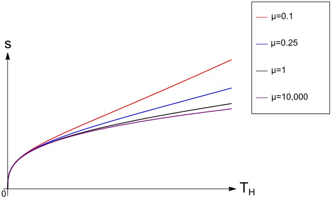
Figure 1: Mathematica plot of (3.40), showing how entropy densitysvaries with temperature

TH for various values of the chemical potentialµ, and with Q0 andZ fixed.

Thermodynamics and the Nernst Law

We are now in a position to relate the integration constantsB0andh0appearing in our solution to the thermodynamic quantitiess,TH andµ. In particular, we can rearrange (3.39) to find

e 2B₀h₀

Q0 = 1 + B0

Q0µ = 1 + 2πsTH

Q0µ

,

where we have used (3.36). Returning to (3.35) we then find an equation determining the entropy density as a function of the electric chargeQ0, fluxesg1, . . . , gn, temperatureTH and

chemical potentialµof the black brane:

s3= 4πZ2TH

1 +2πsTH

Q0µ

. (3.40)

One consequence of (3.40) is that, if we keepZ,Q0andµfixed and sendTH→0, we see that

s_→0, which is precisely the strict (Planckian) formulation of the third law of thermodynamics [9]. This identifies the solution constructed in Section 3.3 as a non-extremal (‘hot’) Nernst brane.

We can further analyse (3.40) by looking at the dimensionless ratio TH/µ. When TH/µ

is small, the second term in (3.40) becomes negligible, and we find that the entropy density behaves ass_∼T_H1/3. On the other hand, whenTH/µ becomes large, the second term in (3.40)

dominates, and we find the behaviours_∼TH.

In Figure 1 we plot equation (3.40) for various values of µ, keepingQ0 and Z fixed. This shows a) the Nernst Law behaviours_→0 asTH →0, and b) the crossover from the behaviour

4

A magnetic black brane

We now turn our attention to a simple reformulation of the procedure in Section 3 which for a certain class of prepotentials allows us to construct non-extremal black branes carrying magnetic charge. We will here simply present the supergravity solution, and leave a fuller discussion of the thermodynamics of magnetically-charged black branes for future work.

In particular, we are interested in prepotentials for which one of the fields Y1, . . . , Yn

de-couples from the others. Without loss of generality, we can assume that Y1 decouples, and consider prepotentials of the form

F(Y) =

_Y1

Y0

˜

f(Y2, . . . , Yn),

where the function ˜f is homogeneous of degree 2. This class is particularly interesting from the perspective of embedding the model into string theory as it contains the tree-level heterotic prepotentials, which are linear in the heterotic dilaton Y1_/Y0_{. We consider black brane} so-lutions which are supported by a single magnetic chargeP1, a magnetic flux g0, and electric fluxesg2, . . . , gn.

In this case we see that the equations of motion can be solved in precisely the same way as in Section 3, with the fieldq1 and magnetic charge P1 playing the role ofq0 andQ0 in the preceding section. In particular, we have

q1(τ) =±P 1

B0 sinh

B0τ+B0

h1

P1

,

whilstq0 andq2, . . . , qn take the same form as (3.20) after replacingg1 withg0 in the obvious place. Moreover, the functionψremains unchanged and, since

eφ=1

2(−q0q1f˜(q2, . . . , qn))

−1 2_,

is symmetric in q0 and q1, we find that the line element takes the same form as in Section 3. Looking at the near-horizon behaviour we again find that regularity of the solution imposes the same relation between the integration constants, a0 = B0, as before. The entropy density is therefore

s=Z1/2(2B0)1/4_eB0h1

2P1 _,

whilst the temperature of the solution is given by

4πTH =Z−1/2(2B0)3/4e−

B0h1

5

Discussion and conclusions

In this paper we have provided a new technique for the construction of non-extremal black brane solutions to large classes of _N = 2 U(1) gauged supergravity models, utilising the techniques of time-like dimensional reduction followed by a rewriting of the effective three-dimensional degrees of freedom through the real formulation of special geometry. In Section 3 we explicitly constructed a family of non-extremal black branes supported by a single electric charge and an arbitrary number of electric fluxes. This family of branes has an entropy density behaving as s _∼ T1/3 for T _→ 0, which therefore vanishes at T = 0, where we recover the extremal Nernst brane solutions of [19]. We anticipate that such non-extremal Nernst branes will have interesting applications in the context of holography, where they could prove useful in describing dual field theory configurations at finite temperature and chemical potential which satisfy the Nernst Law.

One issue with regards to a holographic interpretation is that our solutions do not fit nat-urally into the framework of AdS/CMT, since they do not asymptote to AdS4, but rather conformal AdS4, as seen in (3.37). Hence, the stress tensor of the dual field theory in the UV would not be scale invariant. However, in recent years much progress has been made in understanding the holographic description of such ‘hyperscaling violating’ theories, as well as the more general class of hyperscaling violating Lifshitz (hvLif) theories [4,5,37], which we now review.

Consider spacetime geometries of the form (we use the conventions of [4])

ds2_d+2=r−2(dd−θ)

−r−2(z−1)dt2+dr2+dx2_i, (5.1)

where i = 1, . . . , d label the spatial directions on the boundary, z is the ‘dynamical critical’ (Lifshitz) exponent, andθis the ‘hyperscaling violating’ exponent8_{. Note that forz= 1, θ= 0} one recovers the metric on AdSd+2.

By looking at the near-horizon and boundary behaviour of our solutions, we see that the Nernst brane interpolates between two hvLif geometries (5.1) withd= 2. There are four cases of interest, corresponding to whetherh0 andB0 are zero or non-zero:

• h0 = 0,B0 = 0: The solution becomes globally hvLif (3.33) with (z, θ) = (3,1). It has zero temperature and infinite chemical potential.

• h0= 0,B06= 0: The solution (3.31) has finite temperature and infinite chemical potential, and interpolates between a near-horizon Rindler geometry (3.32), with (z, θ) = (0,2), and an asymptotic hvLif geometry with (z, θ) = (3,1).

It interpolates between a hvLif geometry with (z, θ) = (3,1) at the horizon, and the conformal AdS4 geometry (3.37) with (z, θ) = (1,₋1) at infinity. This is the Nernst brane solution of [19].

• h0 6= 0, B0 6= 0: The solution (3.30) has finite temperature and chemical potential, and interpolates between a near-horizon Rindler geometry with (z, θ) = (0,2) and the conformal AdS4 geometry with (z, θ) = (1,₋1) at infinity.

Note that all of these values are consistent with the constraints imposed by the Null Energy Condition [4]. We have therefore found, analytically, a family of solutions which interpolate between two hvLif geometries. This family is parametrised by the two integration constants

B0 and h0, or equivalently by the temperature T and chemical potential µ of the solution, both of which can be freely varied. Both parameters have a distinct effect on the near horizon and asymptotic forms of the solution: while the extremal or zero temperature limit B0 → 0 changes the near horizon solution from (z, θ) = (0,2) to (z, θ) = (3,1), the infinite chemical potential limith0→0 changes the geometry at infinity from (z, θ) = (1,−1) to (z, θ) = (3,1). If both limits are performed we obtain a global hvLif solution with (z, θ) = (3,1) which we interpret as the ground state of the given charge sector. Note that like any Lifshitz solution different from AdS it is not geodesically complete, and that the scalars are non-constant and run off to zero or infinity in the asymptotic regions. However, a similar behaviour can occur for domain wall solutions in gauged supergravity which, for lack of more symmetric solutions, are interpreted as ground states. Sometimes this interpretation can be further justified by an embedding into string theory or M-theory, see for example [40]. While we leave studying the string theory embedding of our solutions for future work, we remark that the interpretation is consistent with a limit where the temperature is zero and the chemical potential infinite.

Since so far solutions interpolating between hvLif geometries have only been found by relying on a mixture of analytical and numerical methods, we have made a significant step forward, and expect that the techniques used and described in this paper will be useful in making further progress. While we leave searching for a concrete holographic dual of the bulk geometries presented in this paper to future work, we can already make some interesting observations which shed some light on the properties which such a putative dual theory might possess.

Let us first consider the extremal (B0 = 0) solution with h0 = 0. Since this is the grav-itational ground state solution with (z, θ) = (3,1), zero temperature and infinite chemical potential, we expect it to be dual to the ground state of a (2 + 1)-dimensional QFT with hyper-scaling exponentθ= 1 and Lifshitz exponent z= 3. We remark that the specific value θ = 1 for a QFT ind = 2 space dimensions seems to be required for the description of states with hidden Fermi surfaces, although a three-loop calculation givesz=3

the temperature ass_∼Td−zθ =T1/3. We therefore expect that the non-extremal Nernst brane withh0= 0 in (3.31) provides us with the relevant gravity dual to the (2 + 1)-dimensional QFT withθ= 1 andz= 3 at finite temperature. Indeed, takingµ_{→ ∞}in the relation (3.40) we see that the entropy density of the brane solution is related to the temperature ass_∼T1/3 which is the expected behaviour from the field theory arguments, and therefore consistent with our tentative interpretation.

We now move on to consider what happens at finite chemical potential µ < _∞, which corresponds to h0 6= 0. In this case, the extremal Nernst brane interpolates between a hvLif geometry with (z, θ) = (3,1) at the horizon, and a hvLif with (z, θ) = (1,₋1) at infinity, which is conformal to AdS4. One possible interpretation is as an RG flow between two QFTs: one with hyperscaling exponentθ=₋1 in the UV; and one with hyperscaling exponentθ= 1 and Lifshitz exponentz = 3 in the IR. As the gravity solution is smooth, and we do not seem to have a natural candidate for an order parameter identifying a phase transition, we think that the more likely interpretation is that the UV ‘phase’ and the IR ‘phase’ are related by smooth crossover. For the IR theory we expect that the entropy scales like s _∼ Td−zθ = T

1

3, which

agrees with the behaviour of the Nernst brane solution for low temperature T

µ 1. Adding

temperature changes the near horizon geometry, but leaves the asymptotic geometry at infinity unchanged, which is consistent with interpreting these configurations as thermal states. We therefore expect that the IR behaviour is correctly described by the Nernst brane solution, which in turn predicts a scalings _∼T of the entropy for high temperatures, T

µ 1. This however

does not agree with the expected scaling of our tentative UV theory with (z, θ) = (1,₋1), which predicts s _∼ T3. We also note that the asymptotic UV geometry, while conformal to AdS4, cannot be interpreted as an alternative ground state of our supergravity theory, because it is not, when taken as a global geometry, part of our family of solutions. Moreover, the physical scalar fields zA _∼ ρ1/4 run off to infinity in the UV region, which indicates strong coupling or decompactification. Taken together this suggests that the description in terms of our four-dimensional gauged supergravity theory is incomplete in the UV, and that further degrees of freedom become relevant. If we accept that the UV geometry correctly captures the thermodynamic behaviour then the corresponding UV theory should have a scaling behaviour

s

_∼

T

3

in far UV

s

_∼

T

s

_∼

T

µ

T

H

1

Figure 2: The holographic phase diagram for our family of Nernst brane solutions in terms of horizon temperature,TH, and chemical potential,µ, which shows a smooth crossover between

the two scaling regimes. We have also indicated that we anticipate a different scaling behaviour in the far UV where we don’t expect that our supergravity solution accurately describes the tentative dual theory.

Therefore we expect that by lifting our solutions to five dimensions we will obtain new asymp-totically AdS5finite temperature solutions inN = 2 gauged supergravity which still satisfy the Nernst Law9_{. We will expand on this point in [41], and remark that an asymptotic AdS5leads} to a scaling of the entropys_∼Td−zθ =T3, (z= 1, θ= 0, d= 3), which is consistent with our proposed UV theory.

We should also point out that there are issues with the interpretation of our solutions if the temperature is strictly zero, since the Nernst brane solution has infinite tidal forces and run-away behaviour of the scalars at the horizon in the extremal limit. This again indicates a breakdown of the effective description, and strictly speaking the supergravity solution should only be trusted at low but finite temperature. Thus, as in the similar case of the holographic interpretation of hyperscaling violating solutions of Einstein-Maxwell-Dilaton theories [4], the Nernst brane solution is not a valid description of its (tentative) dual over the full range of the energy (radial coordinate) from the UV (infinity) to the IR (horizon), but only over a finite

9_{Although examples of such asymptotically AdS}

interval outside the horizon. We leave it to future work to characterize the range of validity more quantitatively, and to identify the necessary completions in the UV and IR using a string theory embedding. One possible strategy to further investigate the zero temperature limit is to adapt formalisms that allow to include higher derivative terms. InN = 2 supergravity a certain class of higher derivative terms (those encoded in the so-called Weyl multiplet), which are related to the topological string, lead to a generalization of the framework of special geometry, on which we relied in the article [21, 22, 42–45]. One could also try to adapt the entropy function formalism [24], which employs universal properties of near horizon geometries and does not depend on supersymmetry.

Finally we comment on further possible future directions on the gravity side. Here it would be interesting to find solutions where other and possibly more charges and fluxes have been turned on. We expect that our formalism is particularly suited to finding dyonic solutions, due to its built-in electric-magnetic covariance [34]. For work in this direction it is encouraging that work on static BPS solutions inU(1) gauged supergravity solutions with symmetric scalar target spaces has led to the construction of the general dyonic solution [46–49].

We think that the systematic methods and explicit analytical solutions interpolating between hvLif geometries that we have presented in this paper will help to make progress towards a classification of solutions in gauged supergravity, and of the hvLif landscape, and to extend and deepen our understanding of the field theory/gravity dictionary.

Acknowledgements

We would like to thank G. Lopes Cardoso for drawing our attention to the problem of construct-ing non-extremal versions of Nernst branes in gauged supergravity, and for many further useful discussions. We also thank P. Athanasopoulos, M. Haack, S. Gentle, P. Rakow and O. Vaughan for useful discussions. The work of PD is supported by STFC grant ST/J50113X/1 and National Research Foundation of Korea grants 2005-0093843, 2010-220-C00003 and 2012K2A1A9055280. The work of DE is supported by STFC studentship ST/K502145/1. The work of TM is partially supported by the STFC consolidated grants ST/G00062X/1 and ST/L000431/1.

A

Scalar potential in the real formulation of special

ge-ometry

In this appendix we review the real formulation of special geometry introduced in [27], based on the work of [50, 51], and extend it to include scalar potentials of the form (2.3), which result from a flux superpotential (2.4). Starting from the holomorphic formulation, where the complex scalars XI _{parametrise a conic affine special K¨ahler (CASK) manifold, and where all vector}

of degree two, one introduces special real coordinates (qa_{) = x}I_{, y} I

T

, where

XI =xI+iuI, FI(X) =yI +ivI .

Note thatFI =_∂X∂FI is homogeneous of degree one. In the real formulation all vector multiplet couplings are encoded in a Hesse potential H(qa_{), which is homogeneous of degree two, and}

which is obtained from the imaginary part of the holomorphic prepotential by a Legendre transformation, which replacesuI byyI as an independent variable:

H xI, yI

= 2 ImF(X(x, y))₋2yIuI(x, y) =

i

2 X

I_F¯

I(X)−FI(X) ¯XI

. (A.1)

The special real coordinates qa _{are Darboux coordinates, and the K¨ahler form on the CASK}

manifold is simply

dxI _∧dyI =

1 2Ωabdq

a

∧dqb, Ωab=

0 1

−1 0

!

.

It is useful to note that the first derivatives Ha of the Hesse potential are related to the

imaginary parts ofXI _andF I by

Ha= 2(vI,−uI)T,

and provide an alternative, ‘dual’ coordinate system on the CASK manifold.

To obtain the associated projective special K¨ahler (PSK) manifold, one imposes the D-gauge ₋2H = κ−2, together with a condition which fixes a U(1) gauge. If one wants to preserve symplectic covariance, one postpones fixing a U(1) gauge and retains a local U(1) gauge invariance. Geometrically this corresponds to working on the total space of a U(1) principal bundle over the PSK manifold.

In [27] it was shown how to express all couplings appearing in the bosonic part of the vector multiplet Lagrangian in terms of real coordinates. In particular the CASK metric NIJ =

2ImFIJ is replaced by the Hessian metric

Hab=

∂2H ∂qa_∂qb .

For the purpose of this paper we need to rewrite the scalar potential V(X,X¯) of (2.3), and the associated flux superpotentialW(X) of (2.4), in terms of real coordinates. Using that

Ha =Habqbby homogeneity, and using the formulae given above, it is straightforward to obtain

W =W(qa) =W(xI, yI) = 2ga

Ωab+

i

2Hab

qb=iga(Hab−2iΩab)qb, (A.2)

In order to obtain the potential V as given in (2.3), we must compute the derivatives

∂IW =

∂W ∂XI =

1 2

_∂

∂xI −i

∂ ∂uI

W.

Since this derivative involves the real coordinates (xI_{, u}I_{) rather than (q}a_{) = (x}I_{, y} I)T, we

apply the chain rule toW(x, y(x, u)) and compute

∂W ∂xI _u = ∂W ∂xI _y

+ ∂yJ

∂xI ∂W ∂yJ _x

, and ∂W

∂uI _x

= ∂yJ

∂uI ∂W ∂yJ _x .

After decomposing the second derivatives of the prepotential F into real and imaginary parts (including a conventional factor of 2) by 2FIJ =RIJ+iNIJ, one can apply the chain rule to

show that

∂yJ

∂xI =

1

2 FIJ+ ¯FIJ

=1 2RIJ, and read from [27] that

∂yJ

∂uI =−

1 2NIJ. Combining this, we find

∂W ∂XI =

1 2

_∂W

∂xI +FIJ

∂W ∂yJ

, ∂W¯ ∂X¯I =

1 2

_∂W¯

∂xI + ¯FIJ

∂W¯ ∂yJ

.

Finally, we can put all of this together to obtain

NIJ∂IW ∂JW¯ =

1 4Wa

Hab+ i 2Ω

ab

¯

Wb, (A.3)

where (Wa) =

∂W ∂xI,

∂W ∂yJ

T

,Hab_{is the inverse Hessian metric on the CASK manifold (see [27]),}

and Ωab_{is the inverse of Ω} ab.

Using (A.2), we have that

Wa=igb(H−2iΩ)ba, W¯a=−igb(H+ 2iΩ)ba. (A.4)

This can be substituted into (A.3), which after simplification becomes

NIJ∂IW ∂JW¯ =Habgagb, (A.5)

where we have used the identity10_H

abΩbcHcd=−4Ωad[27].

comes from (2.3) using (A.2) and (A.5) as follows:

V =gaHabgb−2κ2ga(Hac−2iΩac)qcgb(Hbd+ 2iΩbd)qd

=gagbHab−2κ2HaHb−8κ2(Ωq)a(Ωq)b

, (A.6)

where we have used homogeneity Ha = Habqb. Lastly, we substitute theD-gauge condition

−2H =κ−2 into (A.6) to obtain

V =gagb

Hab+

HaHb+ 4 (Ωq)a(Ωq)b

H

. (A.7)

Note that the expression within the square brackets is homogeneous of degree zero. This is useful in order to rewriteV in terms of rescaled variables after dimensional reduction.

B

Adapting the real formulation of special geometry to

dimensional reduction

We shall now define the various terms appearing in the three-dimensional Lagrangian (2.6), which uses a modified version of the real formulation of special geometry that is adapted to dimensional reduction. We follow the conventions of [27], to which we refer the reader for further details. Firstly, the complex scalar fields, XI_{, appearing in the four-dimensional}

Lagrangian (2.1), are replaced by rescaled scalars

YI :=eφ/2XI , (B.1)

whereφis the Kaluza Klein scalar. In the four-dimensional theory parametrised by theXI _the

radial direction of the CASK manifold, which is generated by the vector field

ξ=XI ∂ ∂XI + ¯X

I ∂

∂X¯I ,

is a gauge degree of freedom. The above rescaling promotes it to a physical degree of freedom, which is equivalent to the Kaluza-Klein scalar. It turns out that this rescaling leads to a convenient parametrization of the reduced three-dimensional theory. Rewriting the D-gauge condition (2.2) in terms ofYI_{, we obtain}

−i YIF¯I−FIY¯I

=eφ(Y,Y¯), (B.2)

which determinesφin terms of the scalar fieldsYI_.