B R I A N B L A I S
L I F E ’ S M O S T I M P O R TA N T Q U E S T I O N S A R E , F O R T H E M O S T PA R T, N O T H
-I N G B U T P R O B A B -I L -I T Y P R O B L E M S .
P I E R R E - S I M O N L A P L A C E
S TAT I S T I C A L T H I N K I N G W I L L O N E D A Y B E A S N E C E S S A R Y F O R E F F I C I E N T
C I T I Z E N S H I P A S T H E A B I L I T Y T O R E A D A N D W R I T E .
H . G . W E L L S
S TAT I S T I C S A R E T H E H E A R T O F D E M O C R A C Y.
B R I A N B L A I S
S TAT I S T I C A L I N F E R E N C E
F O R E V E R Y O N E
Copyright ©2018Brian Blais
p u b l i s h e d b y sav e t h e b ro c c o l i p u b l i s h i n g
t y p e s e t w i t h t u f t e-l at e x
This book is licensed under the Creative Commons Attribution-ShareAlike license, version4.0,http:// creativecommons.org/licenses/by-sa/4.0/, except for those photographs and drawings of which I am not the author, as listed in the photo credits. If you agree to the license, it grants you certain privileges that you would not otherwise have, such as the right to copy the book, or download the digital version free of charge fromhttp://web.bryant.edu/~bblais. At your option, you may also copy this book under the GNU Free Documentation License version1.2, http://www.gnu.org/licenses/fdl.txt, with no invariant sections, no front-cover texts, and no back-cover texts.
Dedicated to all of the wonderful people at
Bryant University in the Library, Writing
Center, and the Center for Teaching and
Learning who have been exceedingly supportive
Acknowledgements
I would like to acknowledge the following people who have added to this book, in big ways and in small. The book is much better as a result.
Billie Anderson Jim Bishop Jenifer Bond
Paul Campbell Stephanie Carter Allen Downey
Robert Fairhead Rodrigo Fernandez-Vizarra Thomas Hartl
Harold Hausmann Jeremy Hussell Laura Kohl
David Louton Patrick Marchand Alan Olinksy
John Quinn Matt Renfro Steven Rush
Hakan Saraoglu Phillis Schumacher James Scott-Brown
Contents
Proposal
29
1
Introduction to Probability
33
1
.
1
Models and Data
34
1
.
2
What is Probability?
35
Card Game
36
Other Observations
38
1
.
3
Conditional Probability
39
Probability Notation
39
1
.
4
Rules of Probability
40
Negation Rule
41
Product Rule
42
Independence
43
Conjunction
43
Sum Rule
45
Marginalization
46
Bayes’ Rule
47
1
.
5
Venn Mnemonic for the Rules of Probability
49
1
.
6
Lessons from Bayes’ Rule - A First Look
50
2
Applications of Probability
53
2
.
1
Cancer and Probability
53
10
First Solution - Independence
55
Second Solution - Correlation
55
2
.
3
Adding Dice
56
2
.
4
The Birthday Problem
58
Two People on April
3
58
Two People
58
Three People
59
Two People...Out of Three
60
Two People...Out of Thirty
62
2
.
5
The Lottery Problem or Rare Things Are Common
62
2
.
6
Monty Hall Problem
64
Two Doors with Information
65
Three Doors with Information
65
Three Doors Down To Two
66
2
.
7
Exercises
66
2
.
8
Some Philosophical Applications
67
Doctors’ Claims - English Language and Probability
67
Diverging Opinions
68
A problem of independence
69
Another problem with independence
71
Prosecutor’s Fallacy
72
2
.
9
Computer Examples
72
Coin Flips
72
3
Random Sequences and Visualization
75
3
.
1
Coin Flipping
75
Counting the Rearrangements
78
Sequences of Heads and Tails
79
3
.
2
Binomial Distribution
82
3
.
3
Some Philosophical Applications
82
Streaks
82
Gambler’s Fallacy
83
The Hot Hand - Correlations in Random Sequences
84
11
3
.
4
Visualization of Data
87
Histograms
87
Scatter Plots
90
3
.
5
Computer Examples
92
Histograms
92
Scatter Plot
92
4
Introduction to Model Comparison
95
4
.
1
The High/Low Deck Game
95
What does our intuition say?
95
Before the data - the prior
97
The “easy” question - the likelihood
97
Applying the Bayes’ recipe
98
Drawing the next card
99
Prior information or not?
100
4
.
2
Multiple Hypotheses
102
5
Applications of Model Comparison
109
5
.
1
Disease Testing
109
Consequences
111
5
.
2
M&M’s
112
Updating with other data
113
5
.
3
Psychic Octopi
114
Making a Well Posed Problem
114
The First Model Comparison
116
Furthering the Comparison
117
5
.
4
Monty Hall Problem
117
6
Introduction to Parameter Estimation
121
6
.
1
Bent Coins
121
12
6
.
3
Moving Toward the Continuous
125
6
.
4
MAP and Areas
127
6
.
5
Quartiles
129
6
.
6
Best Estimates
131
6
.
7
Uncertainty in the Best Estimates
133
6
.
8
Marginalization
134
6
.
9
Exercises
134
6
.
10
Computer Examples
135
Beta Distribution Example
135
7
Priors, Likelihoods, and Posteriors
139
7
.
1
Binomial and Beta Distributions
139
7
.
2
The Normal Distribution - Properties
140
The Shape
140
The location parameter,
µ
141
The deviation parameter,
σ
141
Summarizing the Distribution
142
Moving from a General Normal to the Standard Normal and Back
142
Sum and Differences
144
7
.
3
The Normal Distribution - Estimating From Data
146
Estimating the mean,
µ
, knowing the deviation,
σ
146
Estimating the mean,
µ
,
not
knowing the deviation,
σ
148
7
.
4
Normal Approximation
149
The Beta Distribution
149
The Binomial Distribution
151
The Student’s t Distribution
152
7
.
5
Summary
154
7
.
6
Computer Examples
155
13
8
Common Statistical Significance Tests
159
8
.
1
z-test
159
8
.
2
What it means and doesn’t mean
161
Significance
161
8
.
3
Student-t-test
162
8
.
4
Computer Examples
163
9
Applications of Parameter Estimation and Inference
165
9
.
1
Normal Model - Inference about Means
165
9
.
2
Normal Model Again - Inference about Means and Deviations
166
9
.
3
Beta Model - Inference About Proportions
170
9
.
4
Model Construction
173
9
.
5
Computer Examples
180
Iris Example
181
Sunrise
183
Cancer Example
184
Pennies
185
Ball Bearing Sizes
190
10
Multi-parameter Models
193
10
.
1
Simple Linear Regression
193
Mean Squared Error
195
An Educational Example
197
10
.
2
Multiple regression
199
10
.
3
Computer Examples
202
11
Introduction to MCMC
211
11
.
1
One-Dimensional Models
211
Reading the Output
212
11
.
2
Multi-Dimensional Models
213
14
12
Concluding Thoughts
219
12
.
1
Where have we come?
219
12
.
2
Where are we going?
220
Bibliography
221
Appendix A:
Computational Analysis
223
Appendix B:
Notation and Standards
225
B.
1
Useful Greek Letters
225
B.
2
Some Math Notation
225
Variables
225
Sums
226
Products
226
Sample Mean
226
Sample Standard Deviation
227
Estimates
227
Factorials
227
B.
3
Qualitative labels to probability values
227
Appendix C:
Common Distributions and Their Properties
229
C.
1
Discrete and Continuous
229
C.
2
Uniform
229
Discrete
229
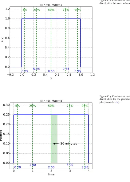
Continuous
229
C.
3
Binomial
232
C.
4
Beta
232
15
Appendix D:
Tables
235
D.
1
Credible Intervals for Standard Normal Distribution
235
D.
2
Credible Intervals for Student’s t Distribution
236
List of Figures
1.1 Standard52-card deck. 13cards of each suit, labeled Spades, Clubs,
Diamonds, Hearts. 36
1.2 Venn diagram of a statement,A, in aUniverseof all possible
state-ments. It is customary to think of the area of theUniverseto be equal to1so that we can treat the actual areas as fractional areas
represent-ing the probability of statements likeP(A). In this image,Atakes up1/4of theUniverse, so thatP(A) =1/4. Also shown is the
nega-tion rule.P(A) +P(not A) =1 or “inside” ofA+ “outside” ofA
adds up to everything. 49
1.3 Venn diagram of the sum and product. The rectangleBtakes up1/8
of theUniverse, and the rectangle Atakes up1/4of theUniverse. Their
overlap here is1/16of theUniverse, and representsP(AandB). Their
total area of5/16of theUniverserepresentsP(AorB). 49
1.4 Venn diagram of conditional probabilities,P(A|B)andP(B|A). (Right)
P(A|B)is represented by the fraction of the darker area (which was originally part ofA) compared not to theUniversebut to the area of
B, and thus representsP(A|B) =1/2. In a way, it is as if the con-ditional symbol, “|,” defines theUniversewith which to make the com-parisons. (Left) Likewise, the same darker area that was originally part ofBrepresentsP(B|A)which makes up1/4of the area ofA.
ThusP(B|A) =1/4. 50
1.5 Venn diagram of mutually exclusive statements. One can see thatP(AandB) =
0 (the overlap is zero) andP(AorB) =P(A) +P(B)(the total area is just the sum of the two areas) 50
2.1 Probability for rolling various sums of two dice. Shown are the
re-sults for two6-sided dice (left) and two20-sided dice (right). The dashed
line is for clarity, but represents the fact that you can’t roll a fractional sum, such as2.5. 57
2.2 Probability of having at least two people in a group with the same
birthday depending on the number of people in the group. The50%
18
3.1 Probability of gettinghheads in30flips. Clearly the most likely value
is15, but all of the numbers from12up to18have significant
prob-ability. 81
3.2 Probability of gettinghheads in30flips given a possible unfair coin.
One coin hasp=0.1, where the maximum is for3heads (or1/10
of the30flips), but2heads is nearly as likely. Another hasp=0.5,
and is the fair coin considered earlier with a maximum at15heads
(or1/2of the30flips). Finally, another coin shown as p=0.8 where 24heads (or8/10of the30flips) is maximum. 83
4.1 High Deck -55Cards with ten10’s, nine9’s, etc... down to one Ace.
Aces are equivalent to the value1. 96
4.2 Low Deck -55Cards with ten Aces, two2’s, etc... up to one10. Aces
are equivalent to the value1. 96
4.3 Drawing a number of9’s in a row, possibly from a High, Low, and
Nines deck. 105
5.1 Rare disease and testing. Shown is a population of3000where1in
every200people have the disease (large circles). A test which is99%
effective is applied to everyone in the population, and the positive test results (i.e. the test says that you have the disease) are shown ask small black dots. Notice that although nearly all of those that have the disease test positive (a small black dot inside a large circle), there are many false positives (black dot in an empty square) - healthy peo-ple that test positive for the disease. Even though the test is quite good, there are many more healthy people and1out of100of them will
erroneously test positive. 111
5.2 The full results of the predictions of Paul the Octopus, reproduced
fromen.wikipedia.org/wiki/Psychic_octopus. 115
6.1 Bent Coins 121
6.2 Probability for different bent-coin models, given the data=9tails,3
heads. 123
6.3 Probability for different bent-coin models, given no data (left), the
first tails (middle), and the second tails (right). The curve for no data is the same as the prior probability, and in this case all models are equally likely. When the first tails is observed, the model which states that heads arecertain(coin10) goes to zero probability. As more tails
are observed, the probability for the lower models is increased. 125
6.4 Probability for different bent-coin models, given three tails (left), the
first heads (middle), and another tails (right). When the first heads is observed, the model which states that heads areimpossible(coin
19
6.5 Probability for different bent-coin models, given no data (left), the
first half of the data set (middle), and the entire data set of9tails and 3heads (right). 126
6.6 Posterior probability distribution for theθvalues of the bent coin
-the probability that -the coin will land heads. The distribution is shown for data3heads and9tails, with a maximum atθ=0.25. 128
6.7 Posterior probability distribution for theθvalues of the bent coin
-the probability that -the coin will land heads. The distribution is shown for data3heads and9tails. The area under the curve fromθ = 0
(the “all heads” coin) toθ=0.5 (the “fair” coin) is0.954. 129
6.8 Posterior probability distribution for theθvalues of the bent coin
-the probability that -the coin will land heads. The distribution is shown for data3heads and9tails. The area under the curve fromθ = 0
(the “all heads” coin) toθ = 0.28 is0.5- half the area. This
repre-sents themedianof the distribution. 130
6.9 Posterior probability distribution for theθvalues of the bent coin
-the probability that -the coin will land heads. The distribution is shown for data3heads and9tails. The various quartiles are shown in the
plot, and summarized in the accompanying table. 131
6.10Posterior probability distribution for theθvalues of the bent coin
-the probability that -the coin will land heads. The distribution is shown for data10heads and20tails. The various quartiles are shown in the
plot, and summarized in the accompanying table. 135
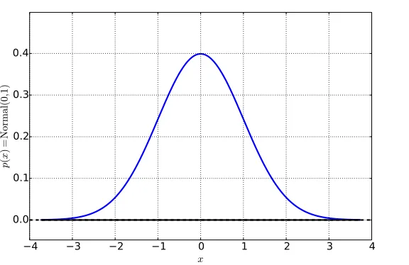
7.1 The Normal Distribution. 140
7.2 The Normal distribution with different location parameters,µ. 141
7.3 The Normal distribution with different deviation parameters,σ. 142
7.4 The Standard Normal Distribution (the Normal distribution in the
special case whereµ = 0 andσ = 1). The percentiles shown are for positions1-σ away from the center,2-σaway, and3-σaway. The
area within1-σis0.68, within2-σis0.95, and3-σis0.99. These
lo-cations are the most prevalently used in any kind of statistical test-ing, and thus we will see them many times. 143
9.1 Probability distributions for the subset of iris petal lengths. Each
dis-tribution follows a Student-t form. 168
9.2 Probability distributions for the difference between iris petal lengths
for the closest two iris types,VirginicaandVersicolor. The distribu-tion follows a Student-t form, and clearly shows significant proba-bility (greater than99%) for being greater than zero. 169
9.3 Mass of Pennies from1960to1974. 174
9.4 Mass of Pennies from1960to1974, with best estimates and99% CI
20
9.5 Mass of Pennies from1960to2003, with best estimates and99% CI
(i.e. 3σ) uncertainty. 179
9.6 Mass of Pennies from1960to2003, with best estimates for the two
true values and their99% CI (i.e. 3σ) uncertainty plotted. There is
clearly no overlap in their credible intervals, thus there is a statisti-cally significant difference between them. 180
9.7 Difference in the estimated values of the pre- and post1975pennies,
µ1−µ2. The value zero is clearly outside of the99% interval of the
difference, thus there is a statistically significant difference between the two valuesµ1andµ2. 181
10.1Heights (in inches) and shoe sizes from a subset of McLaren (2012)
data. 194
10.2Posterior distribution for the slope for the linear model on the shoe
size data subset. 195
10.3Posterior distribution for the intercept for the linear model on the
shoe size data subset. 196
10.4Best linear fit for the shoe size data subset. 196
10.5Minimizing the Mean Squared Error (MSE) results in the best
lin-ear fit for the shoe size data subset. 197
10.6Total SAT score vs expenditure (top) and the distributions for the slope
(bottom left) and intercept (bottom right). 198
10.7Percent of students taking the SAT vs per pupil expenditure (top)
and the distributions for the slope (bottom left) and intercept (bot-tom right). 200
10.8The posterior distributions for coefficients on the expenditure term,
the percent taking term, and the intercept. 201
11.1So-called MCMC “chains” for parameterθversus time. Observe that
the values ofθstart spread evenly from0to1at the beginning and
then thin down to a range of about0.5-0.8with the middle around 0.7(17/25=0.68). 212
11.2Distribution ofθ, and the95% credible interval. 213
11.3Chains for parametersa,b, and the noiseσ. 213
11.4Data (blue) and predictions (green) for the model - the width of the
predictions demonstrates the uncertainty. 214
11.5Distributions for parametersaandb(slope and intercept). 215
11.6Chains for parametermu1, the mean of thedruggroup. 217
11.7Distribution for parametermu1, the mean of thedruggroup. 217
11.8png 218
11.9Distribution for parameterδ, the mean of thedifferencebetween the
druggroup and theplacebogroup. 218
C.1 Discrete uniform distribution for values1to6. The value for each
21
C.2 Continuous uniform distribution between values0and1 231 C.3 Continuous uniform distribution for the plumber example
(Exam-ple C.1). 231
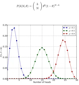
C.4 Probability of gettinghheads in30flips given a possible unfair coin.
One coin hasp=0.1, where the maximum is for3heads (or1/10
of the30flips), but2heads is nearly as likely. Another hasp=0.5,
and is the fair coin considered earlier with a maximum at15heads
(or1/2of the30flips). Finally, another coin shown as p=0.8 where 24heads (or8/10of the30flips) is maximum. 232
C.5 Posterior probability distribution for theθvalues of the bent coin
-the probability that -the coin will land heads. The distribution is shown for data3heads and9tails. The various quartiles are shown in the
plot. 233
List of Examples
1.1 What is the fraction of the first card as a jack given that we know
that the first card is a face card?. . . 41
1.2 What is the fraction of cards that are Jacks and a heart?. . . 42
1.3 What is the probability of drawing two Kings in a row? . . 42
1.4 What is the probability of flipping two heads in a row? . . . 43
1.5 Marginalization and Card Suit . . . 46
1.6 What is the probability of drawing a jack, knowing that you’ve
drawn a face card? . . . 47
2.1 What is the probability of both having cancer and getting a
positive test for it? . . . 53
2.2 What is the probability of both not having cancer and getting
a positive test for it? . . . 54
2.3 What is the probability of having cancergivena positive test
for it? . . . 54
2.4 If the probability that it will rain next Saturday is0.25and the
probability that it will rain next Sunday is0.25, what is the
prob-ability that it will rain during the weekend? . . . 55
2.5 What is the probability of thesumof two dice getting a
par-ticular value, say,7? . . . 56
2.6 What is the probability of rolling a summore than7with two
dice? . . . 57
2.7 What is the probability of rolling various sums with two dice
each with20sides? . . . 57
2.8 Let’s imagine we have the case where two people meet on the
street. What is the probability that they both have April3as
their birthday? . . . 58
2.9 Two people meet on the street, and we ask what is the
prob-ability that they both have the same birthday? . . . 58
2.10 What is the probability that three random people have the same
birthday? . . . 59
2.11 What is the probability thatat least twohave the same
birth-day? . . . 60
2.12 What is the probability thatat least twohave the same
24
2.13 When you have a group of30people, like students in a
class-room, and you ask what the probability of finding two in the room with the same birthday, would your intuition say it is greater or less than50%? . . . 62
2.14 Suppose you’re on a game show, and you’re given the choice
of three doors: behind one door is a car; behind the others, goats. You pick a door, say No. 1(but the door is not opened), and
the host, who knows what’s behind the doors, opens another door, say No.3, which has a goat. He then says to you, "Do
you want to change your choice to door No. 2?" Is it to your
advantage or disadvantage to switch your choice, or does it matter whether you switch your choice or not? . . . 64
2.15 Imagine we have a game with two doors: Behind one door
is a car; behind the other is a goat. You pick a door, say No.
1(but the door is not opened), and the host, who knows what’s
behind the doors, says that there is a90% chance that the car
is behind door No.2. Is it to your advantage to switch your
choice? . . . 65
2.16 The host, who knows what’s behind the doors, points to a door,
choosing the correct door90% of the time and the incorrect
one10%. You pick a door, say No.1, and the host points to
door No. 2. Is it to your advantage to switch your choice? . 65
2.17 Suppose you’re on a game show, and you’re given the choice
of three doors: Behind one door is a car; behind the others, goats. You pick a door, say No. 1(but the door is not opened), and
the host, who knows what’s behind the doors, says that an-other door, say No.3, has a0% chance of having a car, and that
the remaining door (that you haven’t chosen - i.e door No. 2)
has a66% of having the car. He then says to you, "Do you want
to pick door No. 2?" Is it to your advantage to switch your choice?
. . . 65
2.18 Suppose you’re on a game show, and you’re given the choice
of three doors: behind one door is a car; behind the others, goats. You pick a door, say No. 1(but the door is not opened), and
the host, who knows what’s behind the doors, opens another door, say No.3, which has a goat. He then says to you, "Do
you want to change your choice to door No. 2?" Is it to your
advantage or disadvantage to switch your choice, or does it matter whether you switch your choice or not?. . . 66
2.19 Beard and Mustache - An Examination of Independence . . 70
3.1 What is the probability of flipping three heads in a row, with
a fair coin? . . . 75
3.2 What is the probability of flippingthirtyheads in a row, with
25
3.3 What is the probability of flipping two heads in three flips,
with a fair coin? . . . 76
3.4 What is the probability of flipping ten heads in thirty flips,
with a fair coin? . . . 77
3.5 How many ways can we rearrange the unique symbols A, B,
C, and D? . . . 78
3.6 How many ways can we rearrange the symbols A, A, A, and
D? . . . 78
3.7 How many ways are there of rearranging the symbols “A A
A D D”? . . . 79
3.8 What is the probability of flipping ten heads in thirty flips,
with a fair coin? . . . 80
3.9 What is the probability of getting17or more heads in30flips? 81
4.1 What is the probability of drawing a9, given that we know
that we’re holding the High Deck? . . . 97
4.2 What is the probability that you are holding one of either the
High or the Low Deck having drawn five9’s in a row from that
deck? . . . 102
4.3 What is the probability that you are holding one of either the
High or the Low Deck having drawnm9’s in a row from that
deck, wheremstands for a number (m=1, 2, 3,· · ·)? . . . . 103
4.4 What is the probability that you are holding one of either the
High, Low, or Nines Deck having drawnm9’s in a row from
that deck? . . . 104
5.1 Is it better to switch doors? - Monty Hall Problem revisited 117
6.1 What is the best estimate of the probability of a bent coin
flip-ping heads, given the observation of9tails and3heads? . . 132
7.1 Given a Normal distribution with a mean ofµ=150 and a
σ=20, what is the most likely value? . . . 143
7.2 Given a Normal distribution with a mean ofµ=150 andσ=
30, what is the probabilityP(x>170) . . . 143
7.3 We have two Normal distributionsP(x) =Normal(µ=8,σ=
2)andP(y) = Normal(µ = 20,σ = 7). What is the distri-bution forz=y−x? . . . 145
7.4 Estimating the True Length of an Object. . . 147
7.5 Estimating the True Length of an Object...Again . . . 148
7.6 Estimating the True Length of an Object...Yet Again . . . 153
9.1 Iris petal lengths - Best estimate . . . 165
9.2 Iris petal lengths - A different species?. . . 166
9.3 Iris petal lengths - Significantly different? . . . 166
9.4 Ball Bearing Sizes . . . 168
9.5 What is the best estimate (and uncertainty) for each of the two
26
9.6 Is it reasonable to believe that there is a difference in the size
produced between the two lines? . . . 170
9.7 The Sunrise Problem . . . 170
9.8 Cancer Rates . . . 171
9.9 Cancer Rates - Normal Approximation . . . 171
9.10 Will it rain on the4thof July? . . . 172
9.11 Hot Hand Reexamined . . . 172
9.12 Mass of the Penny, Model1- One True Value. . . 173
9.13 Mass of the Penny, Model1- One True Value with More Data176
9.14 Mass of the Penny, Model2- Two True Values . . . 179 C.1 You call a plumber, and they say that they can come anytime
in the next4hours. The probability of them arriving at any
particular time can be represented with a uniform distribu-tion. What is the probability that they arrive in the first20
min-utes of the second hour? . . . 230 D.1 Usage of the Credible Interval Table for the Normal
Distribu-tion . . . 235 D.2 Usage of the Credible Interval Table for the Student’st
List of Tables
1.1 Rough guide for the conversion of qualitative labels to probability
values. 51
3.1 Total Correct Guesses from Students “Predicting” the Results of50
Coin Flips. Shown are the results of a first round and a second round of guessing. 86
3.2 Performance in the Second Round of Students “Predicting” the
Re-sults of50Coin Flips. Shown are the results for those students who
performedbestin the first round (left), and those that performedworst
in the first round (right). 86
3.3 106Male Student Heights (in cm) from a Survey. 88
4.1 Drawingm9’s in a row, from either a High Deck or Low Deck. 104
6.1 Probabilities for flipping heads given a collection of bent coins 121
6.2 Probability for different bent-coin models, given the data=9tails,3
heads. The middle column is the non-normalized value from Bayes’ Rule, needing to be divided byK(the sum of the middle column) to get the final column which is the actual probability. 123
8.1 Rough guide for the conversion of deviations away from zero and
the qualitative labels for probability values for being asignificant de-viation. 161
9.1 Iris petal lengths, in centimeters, for Iris typeSetosa. 165
9.2 Subset of iris petal lengths, in centimeters, for iris typesVirginica,
Se-tosa, andVersicolor. 166
9.3 Production lines are produce a ball bearing with a diameter of
ap-proximately1micron. Ten ball bearings were randomly picked from
the production line (i.e. theFirst line) at one time, and then again for a different production line (i.e. theSecond line). Romano, A. (1977)
Applied Statistics for Science and Industry. 169
9.4 Mass of Pennies from1960to1974. 174
28
10.1Heights (in inches) and shoe sizes from a subset of McLaren (2012)
Proposal
I would like to propose a new introductory statistical inference text-book, which I believe takes a fresh look at a course that fits into nearly every quantitative major at universities.
Initial Motivation
My motivation for this project stems from my dissatisfaction with tra-ditional approaches to the topic, and my belief that there is a better way. A first semester statistics course is generally divided into the following four parts:
I Basic Statistical Concepts
• Basic statistical concepts including population, parameter, sam-ple, and statistic
• Types of data (ordinal, time-series, etc...), and sampling method-ology
• Organizing the data visually or graphically - including his-tograms, pie graphs, box plots, and stem-and-leaf plots • Statistical computations including mean, median, mode,
stan-dard deviation, and percentiles II Probability
• Properties of unions, intersections, conditional probability, independence and mutual exclusivity
• Permutations and combinations • Discrete distributions
• Continuous distributions • Normal distribution
III One-sample Statistics
30
• Sampling distributions
• Computations involving the normal distribution, t-distribution, and binomial distribution (for proportions)
• Hypothesis testing
IV Two-sample Statistics
• Two sample problems - expanding topics from Part III to two variables
Obviously, there is some variability to these topics, but as one can see from most introductory statistics textbooks, there is a consistent approach. My main concerns about the traditional approach can be summarized as follows:
1 Part II (probability) generally covers at least one quarter of the ma-terial in an introductory statistics course. There is a shift from data collection and analysis (Part I) to probability theory. Subsequently, Part III shifts back to a data centered approach and only a small portion of Part II generally applies in Part III. This disconnect be-tween Parts I, II, and III, impedes the learning process. It seems to the students as if the parts are related somehow, but the connec-tion is rarely made. The students are then left with a feeling that the course concerns two completely unrelated topics: probability and statistics.
2 The normal distribution is covered repetitively throughout many chapters of most introductory statistics books. The coverage is included in sections such as: empirical bell-shaped curve (Part I), normal distribution as a type of continuous distribution (Part II), sampling distributions (Part III), interval estimation (Part III), hypothesis testing (Part III), and two population testing (Part IV). There is redundant focus on the normal and t-distributions. These topics are closely related, but not handled cohesively. More importantly, there is little or no discussion of the assumptions of the normal model or how to tell what constitutes “close enough” to normal. In addition, there is generally equal consideration given to the rare practical situation in which the standard deviation is known (and knowing this does not generally alter the result much at all).
31
like a “cookbook”: just find the right recipe for the right problem. The fundamental understanding of statistical inference is under-mined by this approach.
It is my view that the traditional approach detracts from student understanding, with its “cookbook” perspective, disjointed cover-age of probability, and the almost exclusionary focus on the normal distribution.
A New Approach
In the field of statistical inference, there are two primary schools of thought. Each has its proponents, but it is generally accepted that on all problems covered in an introductory course, that both approaches are valid and lead to the same numerical values when applied to actual problems. Only one of these approaches is covered in a tra-ditional course, which denies the students access to an entire field of statistical inference. The traditional approach, also called the fre-quentist or orthodox perspective, leads almost directly to problem (1) above. The other approach, also called Probability Theory as Logic1
, 1
E. T. Jaynes. Probability Theory: The Logic of Science. Cambridge University Press, Cambridge,2003. Edited by G. Larry Bretthorst
derives all statistical inference from probability theory directly. It is this approach that I hope to expose students to in an introductory course.
The probability theory approach to statistical inference has several benefits:
1 All of the same problems as handled traditionally can be handled with this perspective, yieldingexactly the same answers2
. 2
One reason why “Probability theory as Logic” concepts are covered only in advanced courses is the misperception that they are applicable only to more advanced problems, and not applicable to problems normally found in an introductory class. The fact that this misperception exists is a strong argument for a book like this one, to dispel this misperception and to communicate both to students and instructors alike the value of a this approach to basic problems.
2 Statistical inference is theoretically grounded in probability theory, which, although admittedly beyond an introductory course, avoids the “cookbook” approach, where different problems need different methods, that students take away from the traditional textbooks. Here all problems use thesamemethod, derived from probability theory.
3 The reasoning process using the probability theory perspective is more intuitive than the orthodox perspective, especially when dealing with hypothesis testing.
32
In the Probability Theory as Logic perspective, this same calcu-lated value is interpretedexactly like the students’ initial intuition! Thus, testing hypotheses, estimating parameters, and determining uncertainties are far more direct and intuitive using this approach than the traditional approach.
What I Am Proposing
This text can help solve the challenges described above, and more. By focusing on models and data, as opposed to populations and samples, this text can more cohesively bridge the topics described in Parts I, II, and III above. Probability will be introduced as a natural part of solving problems, as opposed to its standalone treatment traditionally done in today’s texts.
In this text, I will use the Probability Theory as Logic approach applied to the same problems that are traditionally covered. This viewpoint can greatly enhance our understanding of statistics and can handle topics such as confidence intervals and hypothesis testing in a very intuitive manner. Statistical inference covered in this way also addresses real-life questions that are not addressed by traditional
statistical methods.3 3
One of the reasons why this ap-proach is usually covered only in more advanced courses is the diffi-culty of the mathematics generally associated with it. Orthodox statis-tics makes heavy use of sampling, which is deemed more intuitive than probability distributions. It is my intention to start with low-dimensional cases, building to distributions, and to augment all concepts with numerical exercises.
Finally, this will be a problem oriented textbook. It is imperative that the problems are cohesive with the pedagogy. I will also plan to use technology, where appropriate, to further student learning and make the textbook more interactive.
1
Introduction to Probability
Life’s most important questions are, for the most part, nothing but probability problems.- Laplace
In1968a jury found defendant Malcolm Ricardo Collins and his wife defendant Janet Louise Collins guilty of second degree robbery1
. 1
J. Sullivan. People v. Collins , 68cal.2d319,1968. URLhttp: //scocal.stanford.edu/opinion/ people-v-collins-22583
The decision hinged on the testimony of bystanders, which stated that the perpetrators had been “black male, with a beard and mous-tache, and a caucasian female with blonde hair tied in a ponytail,” and that they escaped in a “yellow motor car.” A mathematician testified that the oddsagainstthis couple being innocent were one intwelve million, and this was enough for the jury to convict. Later, in an appeal, the California Supreme Court reversed the decision primarily because of lack of evidence, and faulty inference.
In another case, Sally Clark was convicted in1999of the murder of her two young sons2
. Again, the testimony hinged on a statistical 2
Lord Justice Kay. R vs Sally Clark, April2003. URLhttp: //www.bailii.org/ew/cases/EWCA/ Crim/2003/1020.html
argument - the chances of one baby dying in their bed1in8500, so therefore the chances oftwoof them dying in the same way is the square of this, or1in73million. Several years later, and a public statement from the Royal Statistical Society highlighting the erro-neous logic, Sally Clark was released - although she never overcame the resulting damage to her life that the conviction had caused.
We will cover these cases in more detail later, and why the in-ference was faulty, but I introduce the stories here for two reasons. First, is to point out that there are cases in which proper statistical inference can be a life and death matter. Second, it is to highlight the fact that such inference can run counter to one’s intuition. Part of the purpose of this book is to retrain your intuitions and your habits of intuition to avoid such failures.
34 s tat i s t i c a l i n f e r e n c e f o r e v e r yo n e
quantitatively resolve the level of uncertainty, and make valid infer-ences. It is in these cases that statistical inference is most useful.
Statistical inference refers to a field of study where we try to infer unknown properties of the world, given our observed data, in the face of uncertainty. It is a mathematical framework to quantify what our common sense says in many situations, but allows us to exceed our common sense in cases where common sense is not enough. Ig-norance of proper statistical inference leads to poor decisions and wasted money. As with ignorance in any other field, ignorance of sta-tistical inference can also allow others to manipulate you, convincing you of the truth of something that is false.
For example, in1978a Russian satellite deviated from its orbit and became increasingly erratic, and was going to crash into the Earth.3 3
L Heaps. Operation morning light. Paddington, S.l,1978. ISBN 0709203233
This sort of event occurs from time to time, even including a recent
crash of a US spy satellite in2008.4 There was a local news broadcast 4
James Oberg. U.S. satellite shoot-down: The inside story. IEEE Spectrum,2008
about the impending Russian satellite crash which said something like, “the scientists had studied the trajectory of the satellite, and determined that there was only a25% chance of it striking land, and even a much smaller chance striking a populated area.” The report was clearly designed to calm the public, and convince them that the scientists had a good handle on the situation. Unfortunately, given a little thought, one realizes that the Earth’s surface consists of about25% land and75% water, soif you knew nothing about the trajectory of the satellite, you would simply state that it had a25% chance of striking land. Instead of communicating knowledge of the situation, the news broadcast communicated (to those who knew basic statistical inference) that either the scientists were incomplete ignoranceof the trajectory or the reporter had misinterpreted a casual statement about probabilities and didn’t realize what was implied. Either way, the intent of the message and the content of the message (to those who understood basic probability) were in direct conflict.
1
.
1
Models and Data
There are two main aspects of statistical inference: description of data and model analysis. In the description of data, one attempts to summarize a set of data with a smaller set of numbers. Grades in the classroom are summarized by the average, votes in a state are summarized by a percentage, etc... This smaller description of the data is useful for both practical and theoretical reasons. It is more expedient to communicate a small set of numbers than the entire data set, and it is almost always the case that the detailed properties of a set of data are not relevant to the questions that you are asking.
ap-i n t ro du c t ap-i o n t o p ro b a b ap-i l ap-i t y 35
proximate the underlying causes of the data, and unify seemingly unrelated problems. One may have a (mathematical) model for a coin flip which ignores all of the details of the flip, the bounce, and the catch and summarizes the possible results by a single number: the chance that the coin will come up heads. You may then use that same model to describe the voting behavior of citizens during a pres-idential election, or to describe the radioactive decay of particles in a physics experiment. The mathematics is identical, but the interpreta-tion of the components of the model will be different depending on the problem. Modelssimplify, by summarizing data with a small set of causes, and they are used forinference, allowing one to predict the outcome of subsequent events.
The goal of statistical inference is then to take data, and update our knowledge about various possible models that can describe the data. This often means deciding which of several models is the most likely. It can also entail the refinement of a single model, given the new data. All of these activities are closely related to (and perhaps identical to) the methods in science. What we are trying to do is make the best inferences from the data, improve our inferences as new data come in, and plan what data would be the most useful to improve our inferences. In a nutshell, the approach is:
Initial Inference + New Data→Improved Inference
In order to deal with a wide variety of problems, we require a minimal amount of mathematical structure and notation, which we introduce in this chapter.
1
.
2
What is Probability?
Probability theory is nothing but common sense reduced to calculation. -Laplace
36 s tat i s t i c a l i n f e r e n c e f o r e v e r yo n e
struck by lightning sometime in your life isp = 0.0002, or1out of 5000. Statistical inference is simply the inference in the presence of uncertainty. We try to make the best decisions we can, given
incom-plete information. In this book, our approach is to
determine, for each problem, what degree of confidence we have in all of the possible outcomes. The approach of statistical inference covered in this book is about the procedure of most rationally assign-ing various degrees of confidence (which we callprobability) to the possible outcomes of some process using all the objectively available data.
One can think of probability as a mathematical short-hand for the common sense statements we make in the presence of uncertainty. This short-hand, however, becomes a very powerful tool when our common sense is not up to the task of handling the complexity of a problem. Thus, we will start with examples that will perhaps seem simple and obvious, and move to examples where it would be a challenge for you to determine the answer without the power of statistical inference.
Let’s walk through a simple set of examples to establish the nota-tion, and some of the basic mathematical properties of probabilities.
Card Game
A simple game can be used to explore all of the facets of probability. We use a standard set of cards (Figure1.1) as the starting point, and
use this system to set up the intuition, as well as the mathematical notation and structure for approaching probability problems.
Figure1.1: Standard52-card deck. 13cards of each suit, labeled Spades, Clubs, Diamonds, Hearts.
We start with what I simply call thesimple card game5
, which goes 5
i n t ro du c t i o n t o p ro b a b i l i t y 37
like:
simple card game ≡
From a standard initially shuffled deck, we draw one card, note what card it is and set it aside. We then draw another card, note what card it is and set it aside. Continue until there are no more cards, noting each one along the way.
(1.1)
There are certain principles that guide us in developing the math-ematical structure of probability. We start with some common sense notions, written in English, and then write them as general princi-ples. These principles, then, constrain our mathematics so that we can apply the ideasquantitatively.
When asked “what is the probability of drawing a red on the first draw?” you would generally say50-50, or50%, or equivalently written as a probability,P(R1) = 0.5. The reason for this is that
we are completely ignorant of the initial conditions of the deck (i.e. where each card is located in the deck after the initial shuffling). Given this level of (or lack of) knowledge, we could swap the colors of the two suits and we would have an equivalent state of knowledge - the problem would be identical. We will keep coming back to this concept, but in general:
Principle of Knowledge and ProbabilityEquivalent states of Principle of Knowledge and
ProbabilityEquivalent states of knowledge must yield equivalent probability assignments.
knowledge must yield equivalent probability assignments. Because of this principle, we are led to the conclusion that
P(R1) =P(B1)
whereR1represents the statement “a red on the first draw” andB1
represents “a black on the first draw.” Because these are the only two options, and they are mutually exclusive, then they must add up to1. Thus we have
P(R1) =1−P(B1)
which leads directly to our original assignment
P(R1) =P(B1) =0.5
Mutually ExclusiveIf I have a list ofmutually exclusiveevents, then Mutually ExclusiveIf I have a
list ofmutually exclusiveevents, then that means that only one of them could possibly be true. Examples includes the heads and tails outcomes of coins, or the values of standard6-sided dice. In terms of probability, this means that, for events A and B,
P(AandB) =0.
38 s tat i s t i c a l i n f e r e n c e f o r e v e r yo n e
cards. In terms of probability, this means that, for events A and B, P(AandB) =0.
Non Mutually ExclusiveIf I have a list of events that arenot mutu- Non Mutually ExclusiveIf I have
a list of events that arenot mutually exclusive, then it is possible for two or more to be true. Examples include weather with rain and clouds or holding the high and the low card in a poker game.
ally exclusive, then it is possible for two or more to be true. Examples include weather with rain and clouds or holding the high and the low card in a poker game.
Now, this was a long-winded way to get to the answer we knew from the start, but that is how it must begin. We start working things out where our common sense is strong, so that we know we are proceeding correctly. We can then, confidently, apply the tools in places where our common sense is not strong.
In summary, with no more information than that there are two mutually exclusive possibilities, we assign equal probability to both. If there are only two colors of cards in equal amounts, red and black, then the probability of drawing a red isP(R1) =0.5 and the
probabil-ity for a black is the same,P(B1) =0.5.
Other Observations
If instead of just the color, we were interested in the suit (hearts, diamonds, spades, and clubs), then there would be four equal and mutually exclusive possibilities. We have a certain number of possi-bilities, and our state of knowledge is exactly the same if we simply swap around the labels on the cards. If we’re interested in the specific card, not just the suit, the logic is the same. Thus, we have
P(♠) =P(♣) =P(♦) =P(♥)
and for drawing one specific card from the deck,
P(A♠) =P(2♠) =P(3♠) =· · ·=P(K♥)
Further, they all must add up to1, so we get for suits
P(♠) +P(♣) +P(♦) +P(♥) =1
and for the specific card from the deck,
P(A♠) +P(2♠) +P(3♠) +· · ·+P(K♥)
| {z }
52cards
=1
Putting it together, we get for the suits
P(♠) =P(♣) =P(♦) =P(♥) = 1
i n t ro du c t i o n t o p ro b a b i l i t y 39
and for the specific card
P(A♠) =P(2♠) =P(3♠) =· · ·=P(K♥) = 1
52
Probabilities for Mutually Exclusive Events In general, for mutu- Probabilities for Mutually
Exclu-sive Events
P(A) = (number of cases favorable to A) (total number of equally possible cases)
ally exclusive events, we have
P(A) = (number of cases favorable to A)
(total number of equally possible cases) (1.2)
1
.
3
Conditional Probability
It is important to understand that probability reflects our state of knowledge about the system. As our knowledge changes, so do our probability assignments. As we gain more information, we change our probability assignments. Two people observing the same system, but withdifferentinformation about the system, will givedifferent probability assignments. All we need to make sure probability theory matches our common sense is for two people with the same state of knowledge, or the same information, to yield identical probability assignments.
Because our information about a system is so important in assign-ing probabilities, we introduce a way of writassign-ing it mathematically that we will use for the rest of the book. It will be good for the reader to get used to reading the mathematical short-hand in English in order to gain an understanding for what it means.
Probability Notation
In math, we choose to abbreviate long sentences in English, in order to use the economy of symbols. In this book we choose a middle-ground between mathematical succinctness and the ease of under-standing English. We start with the simple card game (Equation1.1)
We then define a new symbol,|, which should be read as “given.” When there is information given we call this probabilityconditional on that information. When we write the following:
P(red on first draw|simple card game) (1.3) or
40 s tat i s t i c a l i n f e r e n c e f o r e v e r yo n e
“The probability of drawing a red on the first draw,given thatwe have a standard initially shuffled deck and we follow the procedure where we draw one card, note what color it is and set it aside and continue drawing, noting, and setting aside until there are no more cards.”
One can easily see that the mathematical notation is far more efficient. It is important to be able to read the notation, because it describes what we know and what we want to know.
Conditional ProbabilityWhen information is given, and ex- Conditional ProbabilityWhen
information is given, and expressed on the right-hand side of the| sign, we say that the probability isconditional.P(I’m going to get wet today|raining outside)is an assessment of how likely it is that I will get wetgiven, orconditional on, the fact that it is raining outside. Clearly this number will be differ-ent if it was conditional on the fact that it is sunny outside.
pressed on the right-hand side of the|sign, we say that the proba-bility isconditional. P(I’m going to get wet today|raining outside)is an assessment of how likely it is that I will get wetgiven, or condi-tional on, the fact that it is raining outside. Clearly this number will be different if it was conditional on the fact that it is sunny outside -different states of knowledge yield -different probability assignments.
Causation. Imagine we have a2-card game: a small deck with one red card and one black card, and I draw a red card first. Clearly this makes the probability of drawing red as the second card equal to zero - it can’t happen. We’re tempted to interpret
P(R2|R1,2-card game) =0
to mean thatbecause we drew a red on the first draw, thiscausesthe impossibility of drawing the red on the second- there is only1red card after all, and drawing it seems tocause
the impossibility of drawing red in the future. However, consider the following:
P(R1|R2,2-card game) =0
which is, if weknewthat the second card we drew was red, then it makes it impossible to have drawn a red card as the first card. This is just as true as the previous case, however, you can’t interpret this as
causation- the second draw didn’t
causethe first draw.
Instead,probability statements are statements of logic, not causation. One can use probabilities to describe causation (i.e.P(rain|clouds)), but the statements of probability have no time component - later draws from the deck of cards act exactly the same as earlier ones.
When we put a comma (“,”) on the right side then we read this as “and we know that.” For example, when we write the following:
P(red on second draw|simple card game,red on first draw) (1.5)
or
P(R2|simple card game,R1) (1.6)
this is short for
“The probability of drawing a red on the second draw,given thatwe have a standard initially shuffled deck and we follow the procedure where we draw one card, note what color it is and set it aside and continue drawing, noting, and setting aside until there are no more cardsand we knowthat we drew a red on the first draw.”
1
.
4
Rules of Probability
From the rule for mutually exclusive events (Equation1.2), we assign
the following probabilities for thefirst drawfrom this deck6 :
6
A face card is defined to be a Jack, Queen, or King. A number card is defined to be Ace (i.e.1) through 10.
• P(10) = 4
52
• P(♥) = 1352 = 14
• P(10♥) = 521
• P(face card) = 1252
i n t ro du c t i o n t o p ro b a b i l i t y 41
It turns out that mathematically, the rules forfractions of things and ofprobabilitiesare the same. Thus, to gain an understanding for the rules of probability, we will calculate fractions (which are more immediately intuitive), and then summarize the same rule for probabilities.
Negation Rule
In this section I’ll use the letterFfor fraction, and we can determine the values simply by counting. The fraction of cards which are hearts
(♥) is Either-or fallacy. The negation
rule, should not be taken to imply that everything is “black and white,” or “there are only two sides to every story.” It really is just a statement of logic, should be carefully considered and has some limitations. For example, the following is true,
P(object is black) +P(object is not black) =1
However, this does not mean the same thing as
P(object is black) +P(object is white)6=1
“Not black” is not the equivalent of “white.” It could be red, or gray, or some other color. A common logical fallacy sometimes referred to as the “either-or fallacy” or the “fallacy of the excluded middle,” turns on this point. Some examples of these fallacies are:
• If we don’t reduce public spend-ing, our economy will collapse. • You’re either with us or you’re a
terrorist.
• Either modern medicine can explain how Ms. X was cured, or it is a miracle.
F(♥) =13
52 = 1 4
The fraction of cards which arenothearts (i.e. the3other suits) is:
F(not♥) = 13×3
52 =
3 4
These numbers add up to one: F(♥) +F(not♥) = 1. We can do this with more complex statements.
F(first card is a face card) = 12
52 F(first card is not a face card) = 40
52 F(first card is a face card) +F(first card is not a face card) = 1 Example 1.1 What is the fraction of the first card as a jack given that we know that the first card is a face card?
We can also apply the negation rule to conditional statements, like “the first card is a jack given that we know that the first card is a face card.” Notice that there are12cards that are face cards, so we restrict our counts to those.
F(jack|face card) = 4
12 =1/3 F(not a jack|face card) = 8
12 =2/3 F(jack|face card) +F(not a jack|face card) = 1
and they add up to one.
Negation Rule Given any information, we have Negation Rule
P(A|B) +P(notA|B) =1
P(statement|information) +P(notstatement|information) =1 or
42 s tat i s t i c a l i n f e r e n c e f o r e v e r yo n e
Product Rule
The product rule comes from looking at the combination of events: event Aandevent B. As before, we’ll work on the numbers from the fractions of the card game.
Example 1.2 What is the fraction of cards that are Jacks and a heart?
This is clearlyF(J♥) = 1/52, but we can look at it a different way that is equivalent. We note that the Jacks constitute4/52of the cards, and thatof those4, only one quarter of them are hearts (one card out of the four cards). So, we can arrive at the fraction of J♥by taking one quarter of the fraction of jacks. So what we have is
F(jackand♥) =F(♥|jack)×F(jack) = 1
4× 4 52 =
1 52
One can equivalently reason from the suit first: the hearts constitute 13/52of the cards, and thatof those13, the Jacks constitute1/13 of the cards. So, we can arrive at the fraction of J♥by taking one thirteenth of the fraction of♥. Again, we have
F(jackand♥) =F(jack|♥)×F(♥) = 1
13× 13 52 =
1 52 In general we have
Product Rule Product Rule
P(AandB) = P(A|B)P(B) = P(B|A)P(A)
P(AandB) =P(A|B)P(B) =P(B|A)P(A) (1.8)
Example 1.3 What is the probability of drawing two Kings in a row?
This is the same as
P(K2andK1)
From the product rule (Equation1.8) we have
P(K2andK1) = P(K2|K1)P(K1)
The second part is straight forward: P(K1) = 4/52. The first part is
asking the probability of drawing a second king, knowing that we have drawn a king on the first draw. Now, there are only51cards remaining when we do the second draw, and only3kings. Thus, we haveP(K2|K1) =3/51 and finally
P(K2andK1) = P(K2|K1)P(K1)
= 3
51× 4 52 =
i n t ro du c t i o n t o p ro b a b i l i t y 43
Independence
As a specific case of the product rule, we can change the rule of the card games such that we reshuffle the deck after each draw. In this way, the result of one draw gives you no information about other draws. In this case, the events are consideredindependent.
Independent EventsTwo events, A and B, are said to be inde- Independent EventsTwo events,
A and B, are said to be indepen-dent if knowledge of one gives you no information on the other. Mathematically, this means
P(A|B) =P(A)
and
P(B|A) =P(B) pendent if knowledge of one gives you no information on the other.
Mathematically, this means
P(A|B) =P(A)
and
P(B|A) =P(B)
In this case, the product rule reduces to the simplified rule for independent events: the product of the individual event probabilities.
Joint Probabilities for Independent Events Joint Probabilities for Independent
Events
P(AandB) =P(A)×P(B)
P(AandB) =P(A)×P(B) (1.9)
We have already seen an example of this, when we looked at drawing the Jack of Hearts: drawing a heart gives you no informa-tion about whether it is a jack, and vice versa. Thus,
P(♥|jack) =P(♥)
Example 1.4 What is the probability of flipping two heads in a row?
The probability of getting “heads” on any given coin flip isP(H) =
0.5. The probability of flipping two heads in a row is then simply P(H1)×P(H2) = 0.5×0.5 = 0.25, because the second flip is
in-dependent of the first. If it wasn’t, then you’d have to determine how the knowledge of the first flip influences our knowledge of the second flip, which is written asP(H2|H1)and the full product rule
(Equation1.8) would need to be used.
Conjunction
44 s tat i s t i c a l i n f e r e n c e f o r e v e r yo n e
terms in the product rule
P(AandB) = P(B|A)
| {z }
less than or equal to 1
×P(A)≤P(A)
In other words, coincidences are less likely than either event hap-pening individually. We intuitively know this, when we make com-ments like “Wow! What are the chances of that?” referring to, say, someone winning the lottery and then getting struck by a car the next day. Sometimes, however, it seems as if one’s intuition does not match the conclusions of the rules of probability. One such case is
called theconjunction fallacy. Combinations of Events and the
English languageI believe that the issue of the conjunction fallacy is more subtle than this. In English, if I were to say “Do you want steak for dinner, or steak and potatoes?” one would immediately parse this as choice between
1 steak with no potatoes 2 steak with potatoes
Although strict logic would parse this choice as
1 steak, possibly with potatoes and possibly without potatoes
2 steak, definitely with potatoes, it is common in English to have the implied negative (i.e. steak with no potatoes) when given a choice where the alternative is a conjunction (i.e. steak with potatoes).
In an interesting experiment, Tversky and Kahneman[Tversky and Kahneman,1983] gave the following survey:
Linda is31years old, single, outspoken, and very bright. She majored in philosophy. As a student, she was deeply concerned with issues of discrimination and social justice, and also participated in anti-nuclear demonstrations.
Which is more probable?
1 Linda is a bank teller.
2 Linda is a bank teller and is active in the feminist movement.
85% chose option2.[Tversky and Kahneman,1974] This, they
at-tributed, to the conjunction fallacy - mistaking the conjunction of two events as more probable than a single event. They went further and did a survey of medical internists with the following
Which is more likely: the victim of an embolism (clot in the lung) will experience partial paralysis or that the victim will experience both partial paralysis and shortness of breath?
Combinations of Events and the English languageIf we interpret the doctor’s choice with this implied negative, we have:
1 clot with paralysis and no shortness of breath
2 clot with paralysis and shortness of breath
and the first one is much less likely, because it would be odd to have a clot and not have a very common symptom associated with it. The doctor’s probability assessment is absolutely correct: both symptoms together are more likely than just one. The “fallacy” arises because the English language is sloppier than mathematical language.
and again,91percent of the doctors chose that the clot was less likely to cause the rare paralysis rather than to cause the combination of the rare paralysis and the common shortness of breath.
Even when correct, the consequence for conjunctions can be mis-used, or at least misidentified. Returning to our example of someone winning the lottery and then getting struck by a car the next day, rare eventsoccur frequently, as long as you have enough events. There are millions of people each day playing the lottery, and millions getting struck by cars each day. We will explore this problem later in Sec-tion2.5, but one immediate consequence is that winning the lottery
i n t ro du c t i o n t o p ro b a b i l i t y 45
Sum Rule
Now we consider the statements of the form AorB. For example, in the card game, what is the fraction of cards that are jacks or are hearts. By counting we get the13hearts and3more jacks that are not contained in the13hearts, orF(jackor♥) = 13+3
52 = 16/52. Now, if
we tried to separate the terms, and do:
F(jack) +F(♥) = 4
52+ 13 52 =
17 52
then we get a number that is too big! It is too big because we’ve double-counted the jack of hearts. Adjusting for this, by subtracting one copy of this fraction, we get
F(jack) +F(♥)−F(jackand♥) = 4
52+ 13 52−
1 52 =
16
52 =F(jackor♥) In general
Sum Rule Sum Rule
P(AorB) =P(A) +P(B)−P(AandB)
P(AorB) =P(A) +P(B)−P(AandB) (1.10)
Sum Rule for Exclusive EventsIf two events aremutually exclusive Sum Rule for Exclusive EventsIf
two events aremutually exclusivethe sum rule reduces to
P(AorB) =P(A) +P(B)
becauseP(AandB) =0 for such events.
the sum rule reduces to
P(AorB) =P(A) +P(B) (1.11) becauseP(AandB) =0 for such events.
So the probability of rolling a1or a2on one die is2/6. One more variant on the Sum Rule is where we have3 propo-sitions. It can be a bit tedious to write it all out, but the end result looks a lot like the original Sum Rule. All we do is break up the terms in pieces, and then apply the Sum Rule to each piece.
P(AorBorC) = P(Aor [BorC])
= P(A) +P(BorC)−P(Aand [BorC]) = P(A) +P(B) +P(C)−P(BandC)−
P(AandBorAandC)
= P(A) +P(B) +P(C)−P(BandC)− [P(AandB) +P(AandC)−
P(AandBandAandC)]
which leads finally to
Sum Rule for Three Events Sum Rule for Three Events
P(AorBorC) = P(A) +P(B) +P(C)− P(AandB)− P(BandC)− P(AandC) + P(AandBandC)
P(AorBorC) = P(A) +P(B) +P(C)−
P(AandB)−P(BandC)−P(AandC) +
46 s tat i s t i c a l i n f e r e n c e f o r e v e r yo n e
In words, when you’re looking for the sum of several events, we add the probabilities (i.e. P(A) +P(B) +P(C)), then subtract the double counting (i.e. P(AandB)) as before. Finally, we need to add back in thetriple count(i.e. P(AandBandC)) because it was taken out too many times with the double count. The accounting here can be somewhat prone to error, but the concepts are always the same: when you add probabilities of events, sayAandB, together the termP(A)includes the probability of bothP(AandB)and the termP(B)includes the probability of bothP(AandB), so you’ve included that probability twice and need to subtract one of them to balance the books. Likewise (although it is harder to show), the first six terms in Equation1.12end up subtracting one too many copies of
P(AandBandC), and we need to add one in at the end.
Marginalization
Another consequence of the sum rule and the product rule is a pro-cess calledmarginalization.
Example 1.5 Marginalization and Card Suit
Imagine we have a number of conditional statements, like:
P(jack|♥) = 1
13 P(jack|♦) = 1
13 P(jack|♠) = 1
13 P(jack|♣) = 1
13
but we are interested in just the probability of drawing a jack, regard-less of the suit, or in our notation
P(jack)
The marginalization procedure for this problem looks like:
P(jack) =
all possibilities
z }| {
P(jack|♥)×P(♥) +
P(jack|♦)×P(♦) +
P(jack|♠)×P(♠) +
P(jack|♣)×P(♣)
= 1
13× 1 4 +
1 13×
1 4 +
1 13×
1 4+
1 13×
1 4
= 4
i n t ro du c t i o n t o p ro b a b i l i t y 47
MarginalizationIf we have a complete set of conditional state- MarginalizationIf we have a
com-plete set of conditional statements, like
P(A|B1),P(A|B2),P(A|B3),P(A|B4),· · ·
then theu