White Rose Research Online URL for this paper:
http://eprints.whiterose.ac.uk/107940/
Version: Accepted Version
Article:
Dughman, S.S. and Rossiter, J.A. orcid.org/0000-0002-1336-0633 (2017) Systematic and
effective embedding of feedforward of target information into MPC. International Journal of
Control. ISSN 0020-7179
https://doi.org/10.1080/00207179.2017.1281439
[email protected] https://eprints.whiterose.ac.uk/
Reuse
Unless indicated otherwise, fulltext items are protected by copyright with all rights reserved. The copyright exception in section 29 of the Copyright, Designs and Patents Act 1988 allows the making of a single copy solely for the purpose of non-commercial research or private study within the limits of fair dealing. The publisher or other rights-holder may allow further reproduction and re-use of this version - refer to the White Rose Research Online record for this item. Where records identify the publisher as the copyright holder, users can verify any specific terms of use on the publisher’s website.
Takedown
If you consider content in White Rose Research Online to be in breach of UK law, please notify us by
International Journal of Control
Vol. 00, No. 00, Month 200x, 1–23
Systematic and effective embedding of feedforward of target information into
MPC
S.S. Dughman∗, J. A. Rossiter∗,
(Received 00 Month 200x; final version received 00 Month 200x)
∗ Department of Automatic Control and Systems Engineering, University of Sheffield, UK, S1 3JD. Email: [email protected], [email protected]
ISSN: 0020-7179 print/ISSN 1366-5820 online c
⃝200x Taylor & Francis
Abstract:Discussions on how to make effective use of advance information on target changes are discussed relatively rarely in the predictive control literature. While earlier work has indicated that the default solutions from conventional predictive control algorithms are often poor, very little work has proposed systematic al-ternatives. This paper proposes an embedding structure for utilising advance information on target changes within an optimum predictive control law. The proposed embedding is shown to be systematic and beneficial. Moreover, it allows for easy extension to deal with more challenging scenarios such as unreachable set points and guarantees of convergence/stability in the uncertain case.
1 Introduction
Model Predictive Control (MPC) has been widely and successfully applied (Qin and Badgwell 2003, Richalet et al. 1978, Fallasohi et al. 2010), primarily because of its ability to handle input and state constraints and multivariable processes in a systematic fashion. Nevertheless, there are some aspects of the algorithm which lack comprehensive systematic approaches and in particular one of these is the effective use of advance information of the target (Goodwin et al. 2011, Dugham and Rossiter 2016). While original work on MPC (Clarke and Mohtadi 1989) argued that advance information was included within the optimisation and therefore assumed this was helpful, it has been noted subsequently (Rossiter and Grinnell 1996, Valencia-Palomo et al. 2014) that in fact this information is often not used systematically and thus can lead to a degradation in performance rather than an improvement.
The reason for this apparent contradiction is relatively simply to understand. In a traditional MPC approach using either open-loop or closed loop predictions (Scokaert and Rawlings 1998, Rossiter et al. 1998), the degrees of freedom (d.o.f.) are focussed on immediate transients. If advance knowledge of the set point changes means that such changes are many samples in the future, these are not contemporaneous with the d.o.f. and thus the d.o.f. are ineffective in using this information (Valencia-Palomo et al. 2014).
The above arguments pertain to the constrained case as well as the unconstrained case. More recent work in the literature has focussed on issues linked to the interaction between set point changes and feasibility (Shead et al. 2010, Ferramosca et al. 2009, Lim´on et al. 2008). Specifically, feasibility issues tend to apply most to dual-mode MPC approaches as these include a terminal constraint, that is, the predicted state nc steps into the future must be within a specified set in order to be sure that the predicted trajectories satisfy constraints. A significant change in the target implies a significant change in the terminal constraint and it may not be possible to find a trajectory that satisfies this terminal constraint, as well as transient constraints; this is denoted as infeasibility. Infeasibility due to target changes can take two forms: (i) the target is infeasible only in transients (Rossiter et al. 1996, Rao and Rawlings 1999, Rossiter 2006, Lim´on et al. 2008) and (ii) the target is permanently unreachable Rawlings et al. (2008), Shead et al. (2010).
optimisation, thus one that can be deployed easily within a standard industrial MPC algorithm.
2 Background on MPC tracking algorithms
This section summarises the key modelling assumptions, notation and some typical MPC algo-rithms in the literature which make use of information about target changes.
2.1 System model and constraints
This paper will use a state space model:
xk+1=Axk+Buk, yk=Cxk+pk (1)
wherexk, yk, uk, pkare states, process output, process inputs and output disturbance respectively at samplek and A, B, C are matrices defining the model. Assume constraints, at every sample, on input and states as follows:
u≤uk≤u; x≤xk≤x (2)
More complex constraints can also be included without any change to the algorithms and con-cepts presented here.
2.2 Performance index
A typical MPC strategy proposes a sequence of candidate future input moves which are expected to give the best predicted performance, where performance is assessed using a defined perfor-mance index. Usually, MPC utilises only the first move of the control candidate sequence and ongoing measurement and optimisation are used to continually improve the planning at each sample. A common performance index (e.g. Rossiter (2003)) penalises the weighted squares of both predicted tracking errors and the control deviations from steady-state, that is:
J =
∞
∑
i=1
(xk+i+1−xss|k+i+1)TQ(xk+i+1−xss|k+i+1) + (uk+i−uss|k)TR(uk+i−uss|k) (3)
where uss|k, xss|k are the estimated steady-states of the input and states which enable y → rk asymptotically,rk being the desired target at sample k. Unbiased definitions ofuss|k, xss|k and their linear dependence on current disturbance estimatepk and targetrk are well known in the literature (e.g. (Muske and Rawlings 1993)) and can be defined for suitableKxr, Kur as follows:
[
xss|k uss|k
]
=
[
Kxr Kur
]
(rk−pk) (4)
Remark 1 : This paper focuses on infinite horizon algorithms due to their superior a priori stability properties. To simplify the presentation of the algebra, the disturbance estimate pk is omitted from the equations hereafter; it is straightforward to include where required and is included in some of the numerical illustrations.
2.3 Degrees of freedom (d.o.f ) and autonomous models for prediction
algorithms the d.o.f can be equivalently parametrised (Rossiter et al. 1998) as perturbationsck about a nominal stabilising control law.
uk−uss|k=−K(xk−xss|k) +ck;i < nc uk−uss|k=−K(xk−xss|k); i≥nc
(5)
The predicted state and input evolution is conveniently captured by combining (1,4,5). Hence, with Φ =A−BK, a one-step ahead prediction model is:
xk+1+i = Φxk+i+ [I −Φ]Kxr(rk+1+i) +Bck
uk+i =−Kxk+i+ [KKxr+Kur](rk+1+i) +ck (6)
It is convenient to describe the predictions (6)using an autonomous model formulation (Kou-varitakis et al. 2000) whose states also include any information available about the d.o.f.ck and the future targetrk at sample k. Such a model is given as follows:
Zk+1 = ΨZk; Zk= [xTk, c→Tk, r→Tk+1]T; Ψ =
Φ [B,0, ..,0] [(Φ−I)Kxr,0, ...,0]
0 Dc 0
0 0 DR
(7)
c
→k=
ck ck+1 .. . ck+nc−1
; r
→k=
rk+1 rk+2 .. . rk+na
; r
→k+2=
0I 0· · · 0 0 0I · · · : : : : : : 0 0 0· · · I 0 0 0· · · I
| {z }
DR
r
→k+1; →ck+1 =
0I 0· · · 0 0 0I · · · : : : : : : 0 0 0· · · I 0 0 0· · · 0
| {z }
Dc
c
→k
(8) Readers will note that within the definitions of DR, Dc assumptions have been embedded into the prediction model thatrk+na+i=rk+na, that is we know the set point onlyna steps into the
future and alsock+nc+i = 0, i≥0 (as required by (5)).
2.4 Admissible sets
The predictions from autonomous model (7) are defined as feasible if they satisfy the constraints (2) for all future samples. For convenience, these constraints are represented as a set of matrix inequalities. Standard algorithms are available in the literature for determining these inequalities (e.g. Gilbert and Tan (1991) or recent variants such as Pluymers et al. (2005a)). At this point it is worth introducing an acronym Maximal Controlled Admissible Set (MCAS) which in this paper is taken to be largest volume region in x-space for which one can determine a choice for d.o.f. c
→ksuch that the predictions of (7) satisfy constraints. In mathematical terms, (for suitable M, N, P, d) the set is denoted as SM CAS where:
SM CAS ={x:∃c
→k s.t M xk+N c→k+P r→k+1 ≤d} (9)
Of particular relevance to this paper is the observation that the MCAS shape and position changes as r
2.5 An Optimal MPC algorithm
A typical infinite horizon MPC algorithm (here denoted as OMPC for optimal MPC) minimises the performance index (3) subject to constraints (9) and using an input trajectory/d.o.f. as specified in (5). Of the optimised c
→k, only the first valueck is deployed and the optimisation is repeated at every sample. This section gives a brief summary of the algebra required for such an algorithm.
The deviations in states and inputs relative to their estimated steady-state values can be expressed in terms of the augmented stateZk as:
xk−xss|k =
[
I,0, ..,0]−[0 0 [Kxr,0,0, ..0]
]
| {z }
Kxss
Zk (10)
uk−uss|k=−
[
K,0, ..,0]−[0 0 [Kur,0, , ...,0]]
| {z }
Kuss
Zk (11)
Substituting (7), (10),(11) into the performance index (3) one can express J in terms of the augmented state as:
J =
∞
∑
i=0
ZkT+i[ΨTKxssT QKxssΨ +KzssT RKzss]Zk+i (12)
It is straightforward to show that this reduces to the following equivalent form:
J =ZkTSzZk; Sz =
∞
∑
i=0
(Ψi)TWΨi (13)
Critically, a simpler method of computing Sz is via a Lyapunov equation so that W = ΨTKT
xssQKxssΨ +KzssT RKzss andSz=W + ΨTSzΨ.
Algorithm 1 : In summary, the OMPC algorithm is given as follows. At every sample, first perform the optimisation:
min c
→k
J =ZkTSzZk s.t. M xk+N c
→k+P r→k+1≤d (14)
Then, use (5) and the first value ck of the optimum c
→k to determine the current system input uk.
In many cases the OMPC algorithm is effective, but it is known to contain a number of weaknesses which are tackled in this paper. Three of these are:
(1) Infeasibility, that is occasions wherexk̸∈SM CAScan occur due to rapid changes inrk, pk and also due to uncertainty. This is more common where the underlying loop control law K is well tuned, which of course is a desirable choice. If xk ̸∈ SM CAS, the algorithm is undefined so an alternative control law is required.
(2) Typical approaches in the literature use na= 1, that is they assume no advance knowl-edge of set point changes. A simplistic inclusion of future information (r
→k+1withna>1)
into the algorithm is often detrimental (Valencia-Palomo et al. 2014).
3 Effective use of advance information assuming feasibility
3.1 Ignoring advance knowledge of the target
Most of the literature using OMPC algorithms ignores advance knowledge of target changes, that is, it tacitly assumes that for the purposes of prediction and optimisation, na = 1 and rk+i = rk+1,∀i > 0. This also means that, within the predictions, xss|k, uss|k are constant. Moreover, it can be shown that (Rossiter 2003) in this case the optimum unconstrained choice of the d.o.f. is c
→k= 0. The proof is not important here, but rather this gives a useful observation which is a helpful insight for the control operator and as we develop the contributions of this paper. When na = 1, that is no advance knowledge, optimisation reduces to minimising the weighted norm of the input perturbations c
→k so the magnitude of→c is a direct indicator of the
impact of constraints on the input choices. If c
→k= 0, constraints are not affecting the choice of control inputs.
3.2 Impact of advance knowledge in the unconstrained case
This section will show that whenna̸= 1, the OMPC algorithm may lose the useful link between the value of c
→k and constraints. Moreover, the section derives the explicit impact of the future target values on the control law (that is the control feedforward term). This is straightforward algebra but is useful hereafter and also gives insight.
Theorem 3.1 : The use of performance index (13) allows the user to formulate the explicit dependence of the control law on future target information.
Proof:The matrix Sz can be decomposed into its individual block elements which show the links between the statesxk, r→k+1, c→k within the cost function:
Sz=
Sx SxcSxr ST
xc Sc Scr ST
xr ScrT Sr
(15)
Use the decomposition of (15) to expand (13):
J =xTkSxxk+ 2xTkSxcc
→k+→c
T
kSc→ck+→r
T
k+1Sr→rk+1+ 2x
T
kSxr→rk+1+ 2→cTkScr→rk+1 (16)
However, it is well known (e.g. Rossiter (2003)) thatSxc= 0. Moreover, within the optimisation ofJ one can ignore the terms based on Sx, Sxr as these contain no d.o.f. and hence:
arg min c
→k
J ≡arg min c
→k
{c
→
T
kSc→ck+ 2→c
T
kScr→rk+1} (17)
Next, minimisingJ w.r.t c
→k one finds:
dJ dc
→k
= 0 ⇒ c
→k=−S
−1
c Scr
| {z }
Pr
r
→k=Pr→rk+1. (18)
Hence, the feedforward term, in the unconstrained case, is given by Pr and the dependence on r
→k+1 is explicit.
Remark 2 : The summation of the block elements of the matrixPrmust be equal to zero. This follows immediately from the observation that if the future target is constant then the optimum unconstrained value is c
→k= 0 and hencePr→rk+1 = 0. This is a useful check for coding errors.
3.3 Potentially negative effects of using advance target knowledge with OMPC and systematic choices for na: the unconstrained case
The results of optimising performance suggested that the optimum value of c
→k depends upon future target values, through the feedforwardPr, and the obvious inference is that one should get better performance by using this information and moreover using as large ana as possible. Surprisingly however, this intuitive expectation is incorrect. In fact, including the feedforward term can cause a deterioration in closed-loop performance as will be shown in this section.
More specifically, this section seeks to give more systematic guidance on how much feed forward information is useful and leads to improved performance and also, what constitutes too much feed forward information which cannot be used effectively and thus can be counter productive. In fact, as the reader will see, the best choice ofna is linked to both the system dynamics and nc.
This subsection demonstrates a trial and error method (Algorithm2 (Dugham and Rossiter 2016)) and a short cut algorithm (algorithm3) to select the best amount of the advance knowl-edge for different systems. While this may seem somewhat simple or lacking rigour, both have the advantage of being easy to code/implement in practice which is a core aim of this paper contribution and moreover gives insights that allow easy extension to the constraint handling case.
Algorithm 2 : For values na from 1 to ny, simulate the process (for a specified target) and compute the runtime cost J using performance index (3) by summing terms over the entire runtime (until all terms have converged to zero). Plot the runtime cost vsna. Select the smallest na giving an acceptable runtime cost on the basis that a smallernamay be preferable if the loss in performance is minimal compared to a largerna.
Algorithm 3 : Determine the closed-loop settling-time ns using a measure such as settling to within 10% of steady-state. Choosena =n∗a=nc+ns/2.
The following examples demonstrate how easily these algorithms can be applied and moreover, the fact that the optimum answer is highly dependent on both closed-loop dynamics and nc. Consider the following systems:
A=
[
0.8 0 0.2 0.2
]
, B=
[
0.2 0.8
]
; C=[1.9−1] (19)
A=
[
1−0.09 1 0
]
, B=
[
1 0
]
; C=[1−0.1] (20)
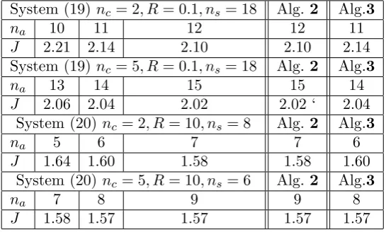
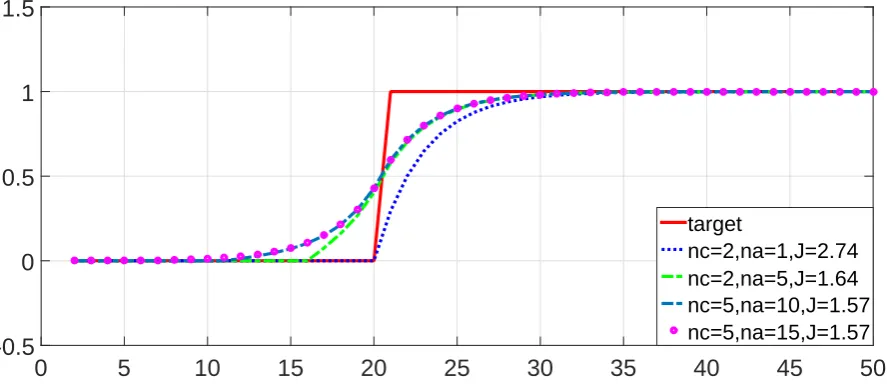
In both cases, closed-loop simulations are performed with a range of values of nc, na. The responses for model (19) are in figure 1 and for model (20) are in figure 2. Table 1 also summarises the performance using runtime cost (3). In summary:
(1) It is clear that advance information can be used systematically and affects behaviour. (2) Up to a limit, choosing na >1 improves performance compared to na = 1 but if na is
Table 1. Variation of performance indices for step changes in target over the runtime for a range ofnaand comparison to proposals
from Algorithms (2,3).
System (19) nc = 2, R= 0.1, ns= 18 Alg.2 Alg.3
na 10 11 12 12 11
J 2.21 2.14 2.10 2.10 2.14
System (19) nc = 5, R= 0.1, ns= 18 Alg.2 Alg.3
na 13 14 15 15 14
J 2.06 2.04 2.02 2.02 ‘ 2.04
System (20) nc = 2, R= 10, ns= 8 Alg.2 Alg.3
na 5 6 7 7 6
J 1.64 1.60 1.58 1.58 1.60
System (20) nc = 5, R= 10, ns= 6 Alg.2 Alg.3
na 7 8 9 9 8
J 1.58 1.57 1.57 1.57 1.57
(3) It is possible to use trial and error (Algorithm2) to choose an optimum value ofnafor a given set point profile but this would cumbersome to implement in practice whereas the simple guideline of n∗
a≈nc+ns/2 suggested by Algorithm3is seen to be fairly effective in the unconstrained case and would be easier to deploy in general.
0
5
10
15
20
25
30
35
40
45
50
-0.5
0
0.5
1
1.5
target
[image:10.595.71.511.328.524.2]nc=2,na=1,J=2.74 nc=2,na=5,J=1.64 nc=5,na=10,J=1.58 nc=5,na=15,J=1.56
Figure 1. Closed-loop step responses for system (19) with variousna, nc.
3.4 Optimising and embedding the use of feed forward information
Before consideration is given to the constrained case, it is important to get the unconstrained case right as this will be the foundation for including constraints later. The previous section and some earlier work (Valencia-Palomo et al. 2014) gave an indication of a possible start point which is to determine the feedforward termPrseparately from the online optimisation, that is to determine a choice ofPr which is known to be optimal in the unconstrained case; such a choice would depend on assumptions about the dynamics with the feedback loop and choices for both na, nc.
0
5
10
15
20
25
30
35
40
45
50
-0.5
0
0.5
1
1.5
target
[image:11.595.67.511.61.256.2]nc=2,na=1,J=2.74 nc=2,na=5,J=1.64 nc=5,na=10,J=1.57 nc=5,na=15,J=1.57
Figure 2. Closed-loop step responses for system (20) with variousna, nc.
Theorem 3.2 : Minimisation of performance index (17) gives the same optimum c
→k as the following optimisation.
˜ c
→= arg min˜c →
˜ J = ˜c
→kSc→c˜k; →ck= ˜→ck+Pr→rk+1 (21)
Proof:A parameterisation of the input perturbationsck which includes the optimum feedfor-ward (18)) and further d.o.f. for constraint handling can be defined as:
c
→k= ˜→ck+Pr→rk+1 (22)
Hence the term ˜c
→kis the deviation from the unconstrained optimum. The cost function is given by substituting (22) into (17). Hence
J ≡[ ˜c
→k+Pr→rk+1]
TSc[ ˜c
→k+Pr→rk+1] + 2[ ˜→ck+Pr→rk+1]
TScrr
→k+1 (23)
From (18) it is known that the unconstrained optimum choice is ˜c
→k = 0 and therefore the performance index must be a quadratic with no-affine term. Therefore, for some constantC,
J = [ ˜c
→k] T
Sc[ ˜c
→k] +C (24)
which implies minimisingJ and minimising ˜J must give the same ˜c
→k. ⊔⊓
Corollary 3.3 : An equivalent MCAS for control perturbations (22) is straightforward to con-struct. This follows directly from substitution of (22) into (9).
M xk+N c
→k+P r→k+1 ≤d ⇒ M xk+N[ ˜→ck+Pr→rk+1] +P r→k+1≤d (25)
Now the constrained optimisation can focus on the computation of just ˜c
Algorithm 4 : The constrained OMPC algorithm with systematic incorporation of advance knowledge can now be summarised as:
min ˜ c
→
˜ J = ˜c
→
T
kSc→˜ck s.t. M xk+N→c˜k+ [N Pr+Q]→rk+1≤d (26)
The optimised ˜ck is used in conjunction with (22,5) to determine uk.
3.5 Summary
The key point here is that, the default OMPC algorithm has the nice property that a choice of c
→ = 0 implies that the unconstrained optimal is feasible and thus one has a clear view on
the impact of constraints as there is a direct link to the magnitude of c
→. However, including
advance knowledge destroyed this link (see eqn.(22)). By re-parameterising the degrees of free-dom in terms of ˜c
→ this nice property is recovered and moreover, the nominal optimal solution,
incorporating advance knowledge, is embedded within the predictions. Hence the required on-line optimisation, a standard quadratic program (QP), is solely dealing with constraint handling and not trying to achieve mixed objectives of performance optimisation and handling advance information alongside constraint handling.
4 Unreachable targets and advance knowledge
The previous section focussed on effective use of advance knowledge when target changes are feasible so that optimisation (26) always has a solution. This section extends the discussion to scenarios where infeasibility occurs, that is, where the change in the steady-state xss|k, uss|k is too rapid, so the prediction class (5) is not sufficiently large to meet constraints. Infeasibility can take two common forms:
(1) Transient infeasibility. That is, the target is reachable asymptotically but a much larger nc is required (Rao and Rawlings 1999) to find a feasible solution. Assuming nc cannot be increased, an alternative algorithm is needed to maintain feasibility and convergence. A common proposal (Rossiter et al. 1996, Rossiter 2006, Lim´on et al. 2008, Shead et al. 2010)) is to include extra d.o.f that capture changes in the steady state. A contractive constraint may be deployed to ensure convergence.
(2) Persistent infeasibility or so called unreachable targets (Shead et al. 2010, Rawlings et al. 2008). In this case, the target cannot be reached, even asymptotically, without violating some constraints and thus an alternative parameterisation allowing changes to the target steady-state is needed, again along with a modified objective.
A key point to note here is that the majority of the work in the literature tackling these two issues assume that na = 1; in this paper proposals are given which embed advance knowledge (i.e. na > 1) while also taking account of transient or permanent infeasibility and moreover, while retaining a simple QP based optimisation.
4.1 Input parameterisation for unreachable targets
In the case where the asymptotic target is unreachable, then the input parameterisation of (5) is invalid, that is, infeasible. The proposal here is to replace this parameterisation with:
uk+i−uss|k+i =−K(xk+i−xss|k+i) +ck+i, i≤nc
uk+i−uss|k+i =−K(xk+i−xss|k+i) +c∞ i > nc (27)
Lemma 4.1 : The inclusion of the term c∞ within the input parameterisation of (27) leads to
a constant offset between the predicted steady-state output and the desired target.
Proof: Substitute the asymptotic input parameterisation of (27) into the model dynamics (1,4). It is clear that ifc∞= 0 there is no offset and hence
lim
k→∞xk=xss=Kxrrk+na ⇒ klim→∞yk=rk+na (28)
Using superposition one can then determine that with (27)
lim
k→∞yk =rk+na+δy∞; δy∞= [C(I−Φ)
−1B]−1
| {z }
G∞
c∞ (29)
Corollary 4.2 : The inclusion of c∞ is equivalent to deploying an artificial target rˆ which is
deviated from the true target byδy∞. Hence, one can also find an equivalent c∞ for a specified
artificial target ˆr as follows:
c∞=G−∞1(ˆrk−rk+na)) (30)
Lemma 4.3 : Minimising performance index (3) with with input parameterisation (27) and na = 1 gives the same optimising values for ck as minimising the following cost:
Jc= c
→
T
kS c→k+
∞
∑
i=1
cT∞Sc∞ (31)
Proof:Minimising the true performance indexJ has been shown earlier (Theorem 3.1) to be equivalent to minimising:
Jc =
∞
∑
i=0
cTk+iSck+i (32)
Then, noting that in effect parameterisation (27) implies ck+nc+i =c∞, i > 0 the result drops
out. The r
→k+1 has been excluded fromJc because herena= 1.
Corollary 4.4 : Combining input parameterisation of (27) with the observation of Theorem 3.2 and Lemma 4.3 one can form an equivalent cost function for na >1 of the form:
˜ Jc≡ ˜c
→
T
kS→c˜k+
∞
∑
i=1
cT∞Sc∞ (33)
Equivalent means the optimum control law from minimisingJc˜ is the same as the optimal control law from minimising Jc.
added in such a way that gives clarity to the impact of constraints in that, the optimised values of ˜
ckare zwero, if and only iff the unconstrained optimal is feasible. Nevertheless, a more significant contribution is to show how optimal trajectories, which include advance knowledge of targets, can also be embedded effectively. The ˜c
→ terms indicate the deviation from the unconstrained
optimal, with advance knowledge, during transients and the c∞ term gives the deviation from
the unreachable target.
4.2 Objective function with steady-state offset
It is well recognised (Rossiter et al. 1996, Rawlings et al. 2008) that the performance index of (33) is not useful in itself because wheneverc∞̸= 0 thisJc is unbounded and hence minimising
Jc is equivalent to minimising the offset component ofcT∞Sc∞. Indeed one could choose simply
to do that, but such an objective would effectively ignore the impact of transient behaviour on overall performance and thus may lead to relatively poor decisions. Consequently, there is a need for a performance index which captures the following requirements:
(1) Has an objective measure of transient performance.
(2) Is always feasible and thus includes the d.o.f. c∞ to allow deviation from unreachable
asymptotic targets.
(3) Includes advance information about target changes.
The key proposal here is to build on the performance index of (33) which already includes transient performance and implicitly has included information about advance knowledge through the deployment of ˜ck. However, we desire a reduced emphasis on the asymptotic predicted error so that this does not swamp the transient terms.
A performance index Jp which gives a balance between transient behaviour and expected asymptotic offset is:
Jp=W1(cT∞Sc∞) + ˜→cTkS→c˜k (34)
where W1 is a weighting matrix to be selected. Here, the term (cT∞Sc∞ penalises asymptotic
offset and the term ˜c
→
T
kS→˜ck penalises transient performance, including information on →rk+1.
The weightingW1 allows the user to determine the emphasis they wish to place on each term.
4.3 Constraint handling
The dynamics now include an additional term as compared to (7), that is the term ck+nc+i =
c∞, i ≥ 0 and hence the autonomous model and inequalities capturing constraint information
need minor modifications to include this. Define the autonomous prediction model as follows:
Zk+1= ΨZk; Ψ =
Φ [B,0, ..,0] 0 [(Φ−I)Kxr,0,0...,0]
0 Dc Ec 0
0 0 I 0
0 0 0 DR
; Zk= [x
T k,→˜c
T
k, c∞, r−→ T k]
T (35)
Dc, EC are shift matrices for ˜ck, c∞ analogous to that in (8).
Using model (35) it is straightforward to apply the admissible set algorithm (Pluymers et al. 2005a) to find a the new MCAS (denoted SM CASU for MCAS Unreachable) of the following format:
SM CASU ={x:∃( ˜c
However, readers should note that a standard admissible set algorithm may not terminate in finite or reasonable time due to the implied steady-state being on a constraint boundary by virtue ofc∞̸= 0 and thus some termination condition needs to be added.
The proposed OMPC algorithm can now be summarised.
Algorithm 5 : An OMPC algorithm with both advance knowledge handling and the potential to manage unreachable targets is summarised in the following optimisation.
min ˜ c
→,c∞
W1(cT∞Sc∞) + ˜→cTkS→˜ck s.t. ( ˜→ck, c∞)∈SM CASU (37)
Use the optimised ˜c
→in conjunction with (22) to determine ck and implement the first moveuk
of the control law as defined in (27).
4.4 Guarantees of feasibility and performance
This section establishes that algorithm5 has guarantees of recursive feasibility and asymptotic convergence to a point which minimises the weighted offset.
Lemma 4.5 : The proposed OMPC algorithm 5 with advance knowledge handling maintains feasibility irrespective of changes in the target.
Proof: The proof follows in a straightforward fashion from the assumption of feasibility at start up and the inclusion ofc∞. If there were no change in target, that isrk+na+1 =rk+na, then
one can use standard MPC arguments to show that the optimum (assumed feasible) solution from samplekcan be carried forward to samplek+ 1 and thus feasibility is retained. In the case whererk+na+1̸=rk+na, one can always introduce a non-zero value ofc∞ such that the implied
artificial target ˆrk+na+1=rk+na, thus again retaining feasibility.
Theorem 4.6 : The proposed algorithm 5 is convergent to the point which minimises the weighted offset.
Proof:At steady-state the optimised values for ck are all identical and therefore the optimi-sation is capped by:
min c
→k
,c∞
Jp ≤cT∞[(W1+nI)S]c∞ (38)
Any optimised value of ck such that cTkSck < cT∞Sc∞ would be a contradiction of the system
being in steady-state and thus, noting the relationship of (30), the optimisation has minimised a weighted norm of the offset.
It is not the purpose of this paper to consider guarantees in the presence of disturbances as that case is altogether much more demanding. The focus here is on a simple approach to deal with the basic requirements. However, it is worth noting that the flexibility afforded in c∞ is
often sufficient to deal with any transient infeasibility caused by changes in disturbances.
4.5 Numerical example with an unreachable target
This section gives numerical examples which demonstrate the efficacy of algorithm5for handling both advance knowledge and unreachable targets in a single simple optimisation.
Table 2. Performance indices for step changes in target for example system (39) using Algorithm5. J with na= 1 J withna= 3 J withna= 5
Example (39) 42.05 38.62 31.92
in a systematic fashion, thus improving performance compared to more conventional approach withna= 1.
Consider the system and constraints
A=
[
0.8 0.1
−0.2 0.9
]
, B=
[
0.1 0.8
]
; C=[1.9−1]; −1≤u≤1.35;
[ −0.8
−2.5
] ≤x≤
[
4 4
]
(39)
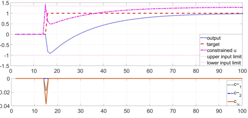
withr= 1, nc = 2, na= 1, R= 0.1I, Q=CTC.
• Figure 3 shows responses when the target is reachable in steady-state, but not in transients, with the use ofna= 1.
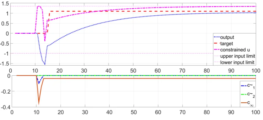
• Figure 4 shows responses when the target is reachable in steady-state, but not in transients, with the use ofna= 5.
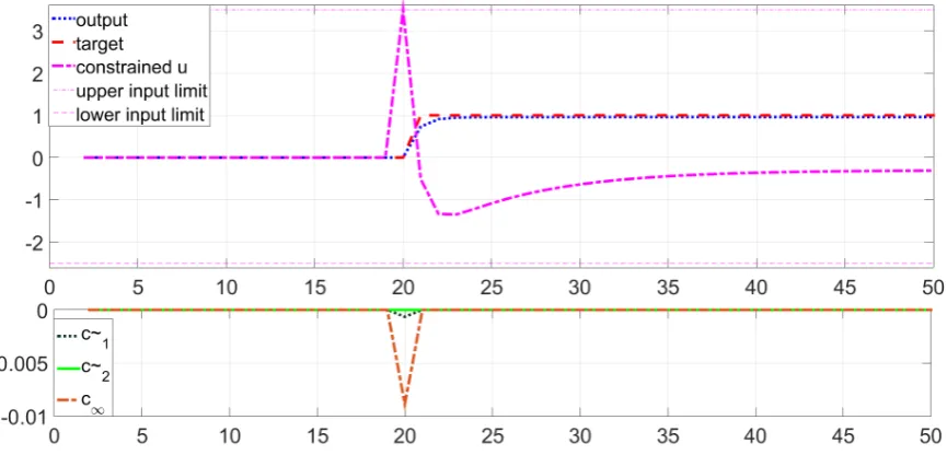
• Figure 5 shows responses when the target is unreachable (now r = 1.1) in steady-state with the use ofna= 5.
It is clearly shown in figures 3, 4 and table 2 that algorithm 5 provides effective control for a constrained system both with no advance knowledge (na = 1) and with advance knowledge. Readers will note that for figures 3,4 the term c∞ (lower figure) is non-zero during transients
only, as expected whereas it remains non-zero permanently in figure 5. The term ˜ck is also non-zero demonstrating the benefits of incorporating advance information systematically, even within these challenging scenarios.
Figure 3. Closed-loop step responses for system (39) using Algorithm5for unreachable target in transient withna= 1.
5 Robust MPC with tracking
[image:16.595.69.499.388.594.2]Figure 4. Closed-loop step responses for system (39) using Algorithm5for unreachable target in transient withna= 5.
Figure 5. Closed-loop step responses for system (39)using Algorithm5for unreachable target in steady state forna= 5.
MPC often require much more demanding algebra and optimisations (Cheng and Jia 2004, Rakovic and Mayne 2005, Chisci et al. 2001).
The proposal here is to build on the robust invariant set approach developed in Pluymers et al. (2005a) and later demonstrated to be effective with a simple dual mode MPC algorithm for regulation Pluymers et al. (2005b). This section will demonstrate how the basic approach can be extended to cater for both tracking scenarios and unreachable set points.
5.1 LPV system model and input predictions
Consider the discrete time LPV system
[image:17.595.62.516.306.513.2]A(k), B(k) are matrices defining the model. Parameter uncertainty is quantified with [A(k)B(k)] ∈ Ω = Co{[A1B1], ....,[AmBm]}, where Co refers to convex hull of the extreme
models, in which [A B]∈Ω, hence with 0≤λi≤1, ∑λi= 1 and [A B] =∑Li=1λi[AiBi]. The dual-mode predictions for system (40) with control law (27) can be described as:
xk+1 = Φ(k)xk+ [I−Φ(k)]Kxr(rk+1) +B(k)ck
uk=−Kxk+ [KKxr+Kur](rk+1) +ck (41)
where Φ(k) =A(k)−B(k)K. It is noted that [A(k)B(k)]∈Ω ⇒ Φ(k)∈Co{Φ1, ....,Φm}.
5.2 The state feedback controller K
It is common in the robust literature (Kothare et al. 1996) for the state feedback controller K to be determined on line so that K is varying every sample. The aim here is to combine this with the ideas summarised in the previous section and maintain algorithm simplicity and thus here assume that K is fixed (for example as in Kouvaritakis et al. (2000)). Nevertheless (Pluymers et al. 2005a) there must exist an invariant set for the uncertain unconstrained closed-loop dynamicxk+1= Φ(k)xk. This can be checked using the following condition.
∃P =PT >0 s.t. ΦiTPΦi≤P, i= 1, ...., m. (42)
Algorithms for identifying aK to satisfy (42) and simultaneously optimise a nominal cost func-tion are readily available but one could equally argue that the correspondingK for the nominal case may also be preferred, if it satisfies (42).
5.3 The closed loop dynamics
It is important to capture the variability in the closed-loop trajectories due to the uncertainty in the model parameters. One can capture this uncertainty efficiently with a set of linear inequalities (Pluymers et al. 2005a), as long as the dynamics and constraints can be captured in appropriate form. The basic algorithm requires a one step ahead state evolution equation (analogous to (35)) and a statement of constraint dependence on the state at each sampling instant.
Lemma 5.1 : The uncertain system predictions of (41) can be captured in a single mode au-tonomous model of the following form.
Zk+1 = Ψ(k)Zk; Zk= [xTk,→˜c T
k, c∞, r−→ T k]
T; Ψ i =
Φi [Bi,0...,0] Γi.G∞ Γi
0 DC EC 0
0 0 DR 0
0 0 0 DR
(43)
where Γi = [Bi,0, ...,0]P r+ [(Φi−I)Kxri,0, ..,0] and Ψ(k)∈Co{Ψ1, ...Ψm}. These predictions are stable and must converge to the specified artificial target of rˆ.
Proof: The definition of Ψi is analogous to (35). Quadratic invariance of the closed-loop dynamic Φ(k) is sufficient to ensure the quadratic invariance of the augmented dynamic Ψ(k) as the additional dynamics in Ψ(k) as compared to Φ(k) relate to the variables ˜c
→k, c∞, r→k. These dynamics are governed solely by shift matrices and thus must converge to fixed, possibly non-zero, values. The asymptotic control law is defined as uk−uss = −K(xk−xss) +c∞ and by
definition c∞ is the value that ensures the associated steady-state output is ˆr (if c∞ = 0 then
5.4 The derivation of a robust MCAS
It is shown in Pluymers et al. (2005a) that one can define a robustly invariant set to guarantee robust stability for the regulation case. This paper extends this set for tracking scenario by deploying a similar concept but with the autonomous model of (43) which includes as states both the degrees of freedom ˜c
→k and also the future target values →rk, c∞. A major difference is convergence to a non-zero steady-state.
Lemma 5.2 : : Constraints at each sample instant can be summarised with the following in-equalities:
GZk≤f (44)
for appropriate G, f.
Proof: This follows from a straightforward substitution from all constraint equations such as (2) and expression in terms of state variable Zk. The definitions of G, f, one row for each constraint, follow automatically.
G=
−K [I,0..,0] αi.G∞ αi
K −[I,0..,0] −αi.G∞ −αi
0 0 [0,0..,0, Kuri].G∞ [0, ..0, Kuri]
0 0 [0, ..,0,−Kuri].G∞ [0, ..,0,−Kuri]
C 0 0 0
−C 0 0 0
0 0 [0, ..,0, CKxri].G∞ [0, ..,0, CKxri]
0 0 −[0, ..,0, CKxri].G∞−[0, ..0, CKxri]
0 0 0 I
0 0 0 −I
; i= 1,2,· · · (45)
wheref =[u¯T, uT,u¯T, uT,x¯T, xT,x¯T, xT,r¯T, rT]T andα
i = [1,0, ...,0]P r+[KKxri+Kuri,0, ..,0]
.
Theorem 5.3 : One can deploy the algorithm of Pluymers et al. (2005a) with sample con-straints (44) and autonomous model (43) and the algorithm will converge, as long as condition (42) is satisfied.
Proof:It is known from condition (42) combined with the convergence to fixed values within nc, na steps of states ck, rk, that the predictions of (43) must converge to a fixed steady-state. The algorithm of Pluymers et al. (2005a) shows therefore that asymptotically, adding predictions for higher horizons results in redundant constraints beyond a certain horizon and therefore the algorithm will terminate.
Let the robust MCAS (denotedSRM CAS) be given as:
SRM CAS =
{
x:∃c˜
→k, c∞ s.t M x+N→c˜k+V c∞+P r→k≤d
}
(46)
Readers should note that where the steady-state is on a boundary strict convergence may re-quire a tolerance to be deployed. This will occur with unreachable set points which, by definition, imply the asymptotic steady-state is on a boundary.
5.5 Robust tracking MPC algorithm
Algorithm 6 : Define the performance index as in (34). Define the robust MCAS as in (46). Perform the quadratic programming optimisation:
min c∞,˜c →k
J s.t. M x+N˜c
→k+V c∞+P r→k≤d (47)
Implement the first block element of ˜c
→k in (27) to compute the control law.
Algorithm 6 gives guaranteed convergence and recursive feasibility, including cases of un-reachable set points because, by definition, the satisfaction of RMCAS of (46) ensures recursive feasibility. In consequence, one can use conventional approaches (Rawlings et al. 2008) to show that ck converges to a weighted minimum. Convergence of ˜c
→k implies convergence of the state xk due to condition (42) and dynamics (43).
5.6 Numerical examples
This section demonstrates that the proposed algorithm6is both robust to parameter uncertainty and handles advance information about the target effectively. Conversely, an algorithm which does not embed the parameter uncertainty gives less effective performance and indeed could lose feasibility. For ease of comparison, the paper uses the uncertain system model that was presented in Lim et al. (2014).
A=Co
{[
0.8 0.0 21.8 1.4
]
,
[
0.8 0.0 16.9 1.3
]}
;B =Co
{[
0.0 0.2
]
,
[
0.0 0.2
]}
(48)
The system input/state constraints are:
−2.5≤u≤3.5;
−0.5≤uss≤0.5;
[ −0.5
−5
] ≤x≤
[
0.5 5
]
(49)
A nominal model A = 0.5A1+ 0.5A2 and B = 0.5B1+ 0.5B2 is used to define the feedback
controllerK =[93.58 5.76] as the LQ-Optimal forQ=diag(1,0.01), R= 0.01.
• Figure 6 demonstrates algorithm6 for system (48) with no advance knowledge (na= 1). It is seen that although the target (r = 1) is unreachable during transients (c∞̸= 0), nevertheless
the algorithm performs well and converges to the correct steady-state without any constraint violations.
• Figure 7 presents algorithm 6 with advance knowledge (na = 3). The target is unreachable during transients but again the algorithm performs well handling both the advance target information effectively and avoiding constraint violations. The response is faster compared to the response figure 6 which did not use advance knowledge. Moreover, the response requires less control effort. The performance benefits, of using advance knowledge with the proposed robust MPC algorithm are further evidenced in table 3, which compares the runtime costs.
Figure 6. Closed-loop for step response of system (48) with algorithm6and with no advance knowledge.
Figure 7. Closed-loop for step response of system (48) with algorithm6and with advance knowledge. Table 3. The Run Time costs for Systemna= 1,na= 3.
System (48)nc = 2, R= 0.01
na 1 3
J 1.262 0.256
6 Conclusions
This paper has made three main contributions. Following a brief review of the literature on approaches to tracking within MPC, it is clear that very few papers have utilised advance information on target changes and the common assumption is that no advance information is available.
Figure 8. Closed-loop for step response of system (48) with algorithm6and with advance knowledge for an unreachable target at steady state.
design.
An argument is made that during constraint handling, it is better to construct predictions which embed the default optimal unconstrained feedforward rather than entering the future target values directly. This ensures the optimal behaviour is embedded and gives transparency to the role of the degrees of freedom. The efficacy and simplicity of this approach is demonstrated. At times, the desired target will be unreachable and in such scenarios a default MPC algorithm becomes ill-defined. This paper proposes a simple alternative which caters for both transient and permanent infeasibility in the target without the need to change the algorithm online. Moreover, it has shown how, even in this case, the systematic embedding of advance information is straightforward and beneficial.
Finally, the paper has shown how all the previous contributions can be extended in a straight-forward manner to cater for parameter uncertainty and thus give robust guarantees of feasibility and convergence while utilising a simple QP optimisation online.
References
Aghaei, S., Sheikholeslam, F., Farina, M., and Scattolini, R. (2013). An mpc-based reference governor approach for offset-free control of constrained linear systems. International Journal of Control, 86, 1534–1539.
Cheng, X. and Jia, D. (2004). Robust stability constrained model predictive control. InACC, volume 2, 1580–1585.
Chisci, L., Rossiter, J., and Zappa, G. (2001). Systems with persistent disturbances: Predictive control with restricted. Automatica, 37(7), 1019–1028.
Clarke, D.W. and Mohtadi, C. (1989). Properties of generalized predictive control. Automatica, 25(6), 859–875.
Dugham, S. and Rossiter, J. (2016). Systematic and simple guidance for feed forward design in model predictive control. International Conference on Control Science and Systems Engi-neering.
Fallasohi, H., Ligeret, C., and Lin-shi, X. (2010), “Predictive Functional Control of an expansion valve for minimizing the superheat of an evaporator,”International Journal of Refrigeration, 33, 409–418.
[image:22.595.68.507.54.262.2]with optimal closed-loop performance. Automatica, 45(8), 1975–1978.
Ferramosca, A., Lim´on, D., Alvarado, I., Alamo, T., Casta˜no, F., and Camacho, E.F. (2011). Optimal mpc for tracking of constrained linear systems. International Journal of Systems Science, 42(8), 1265–1276.
Gilbert, E., Kolmanovsky, I., and Tan, K.T. (1994). Nonlinear control of discrete-time linear systems with state and control constraints: A reference governor with global convergence properties. Conference on Decision and Control, 144–149.
Gilbert, E. and Tan, K. (1991). Linear systems with state and control constraints: The theory and application of maximal admissible sets. IEEE Transactions Automatic Control, 36, 1008– 1020.
Goodwin, G., Carrasco, D., Mayne, D., Salgado, M., and Seron, M. (2011). Preview and feedfor-ward in model predictive control: Conceptual and design issues. In18th IFAC World Congress, 5555–5560.
Kothare, M.V., Balakrishnan, V., and Morari, M. (1996). Robust constrained model predictive control using linear matrix inequalities. Automatica, 32(10), 1361–1379.
Kouvaritakis, B., Rossiter, J.A. and Schuurmans, J. (2000), Efficient robust predictive control
Trans. IEEE AC, 45(8), pp1545–1549
Lim´on, D., Alvarado, I., Alamo, T., and Camacho, E.F. (2008). Mpc for tracking piecewise constant references for constrained linear systems. Automatica, 44(9), 2382–2387.
Lim, J. S., Kim, J-S and Lee, Y.I. (2014), Robust tracking model predictive control for input-constrained uncertain linear time invariant systems, International Journal of Control, 87(), 120–130.
Muske, K.R. and Rawlings, J.B. (1993), Model predictive control with linear models, AIChE Journal, 39(2), 262–287.
Pluymers, B., Rossiter, J., Suykens, J., and De Moor, B. (2005a). The efficient computation of polyhedral invariant sets for linear systems with polytopic uncertainty. In ACC, 804–809. IEEE.
Pluymers, B., Rossiter, J., Suykens, J., and De Moor, B. (2005b). A simple algorithm for robust mpc. In IFAC World Congress.
Qin, S. and Badgwell, T. (2003). A survey of industrial model predictive control technology.
Control Engineering Practice, 11, 733–764.
Rakovic, S. and Mayne, D. (2005). A simple tube controller for efficient robust model predictive control of constrained linear discrete time systems subject to bounded disturbances. InIFAC World Congress.
Rao, C.V. and Rawlings, J.B. (1999). Steady states and constraints in model predictive control.
AIChE Journal, 45(6), 1266–1278.
Rawlings, J.B., Bonn, D., Jrgensen, J., Venkat, A., and Jrgensen, S. (2008). Unreachable set-points in model predictive control. IEEE Transactions on Automatic Control, 53(9), 2209– 2215. .
Richalet, J., Rault, A., Testud, J., and Papon, J. (1978), “Model predictive heuristic control: applications to industrial processes,”Automatica, 14, 413–428.
Rossiter, J., Kouvaritakis, B., and Gossner, J.R. (1996). Guaranteeing feasibility in constrained stable generalised predictive control. IEE Proceedings-Control Theory and Applications, 143(5), 463–469.
Rossiter, J. and Grinnell, B. (1996). Improving the tracking of generalized predictive control controllers.Proceedings of the Institution of Mechanical Engineers, Part I: Journal of Systems and Control Engineering, 210(3), 169–182.
Rossiter, J., Kouvaritakis, B., and Rice, M. (1998). A numerically robust state-space approach to stable predictive control stratgies. Automatica, 34(1), 65–73.
Rossiter, J.A. (2003). Model-based predictive control: a practical approach. CRC press. Rossiter, J. (2006). A global approach to feasibility in linear mpc,. Proc. UKACC ICC.
Control, IEEE Transactions on, 43(8), 1163–1169.
Shead, L., Muske, K., and Rossiter, J. (2010). Conditions for which mpc fails to converge to the correct target. In Journal of Process Control, volume 20, 1207–1219.