Application
of
the
Correction
Function
to Improve the Quality of PM Measurements
with Low-Cost Devices
Mariusz Rogulski1, *, and Artur Badyda1
1Warsaw University of Technology, Faculty of Building Services, Hydro and Environmental Engineering, 20 Nowowiejska St., 00-653 Warsaw, Poland
Abstract. Reliable information on the particulate matter (PM) concentration in the air is provided by professional, reference measuring devices. In recent times, however, measuring devices using low-cost PM sensors have been gaining more and more popularity. Low-cost PM sensors are not as accurate as professional devices and can under certain circumstances significantly distort results. Therefore comparative measurements with professional devices and the determination of the corrective function are necessary. The article presents the results of tests on the accuracy of measurements made with the use of such sensors after applying a correction function. The form of the correction function was determined based on several months of comparative tests low-cost sensors with reference device. Then, for a different set of low-cost sensors, a correction function was applied and again, during several months of research, the measurement results were compared with a reference device. This made it possible to determine the real measurement uncertainty of this type of equipment, as well as the need to support measurements using earlier comparative tests. Results showed, that for analysed low-cost PM sensors and correction function measurement error was about 15%.
1 Introduction
The issue of air quality, and in particular, the level of particulate matter (PM) concentrations arouses great interest in many countries. Reliable information on the dust concentration in the air is provided by professional, reference measuring devices. In recent times, however, measuring devices using low-cost sensors have been gaining more and more popularity. It is well-known that low-cost dust concentration sensors are not as accurate as professional devices and can under certain circumstances significantly distort results. To improve the quality of their indications, calibration or correction is usually necessary. A simple calibration may consist in placing the sensor in an environment in which there is a specific type of pollutant at a known concentration, and then adjusting the sensor's readings in such a way that the difference between the pre-established pollutant concentration and the value indicated by the sensor is minimized [1].
If sensors show a significant correlation of the raw results with the reference device in a large sample of data collected under different meteorological conditions, it is possible to significantly improve the compliance of the measurement results from low-cost sensors in relation to the reference device with a relatively simple correction function. Correction of results may be based, for example, on the use of multiple regression, which will take into account measured concentrations of pollutants and additional parameters, such as meteorological conditions. However, the more varied conditions and the longer measurement period, the better calibration quality.
The method of determining the correction functions (also called calibrating function) is relatively poorly researched, as mentioned for example in [2]. The authors of this article, during an eight-month campaign studied the PM2,5 dust concentration measurements generated by the DS-01D-V1 sensors by comparing them to device using the gravimetric method. The results showed that the tested optical sensor overestimated the results more than three times higher. On the basis of a large set of measurements, the authors determined a correction function linearly dependent on the original values of PM2,5 concentrations, temperature and relative humidity. In [3] the authors proposed a calibration function for Alphasense's electrochemical NO2 sensors. After the measurements together with the reference device and the determination of the calibration function, the values of the determination coefficients for the tested set of sensors increased from the source range of 0.3-0.7 to 0.6-0.9 after calibration. In conclusion, the authors stated that measurement campaigns using low-cost sensors based on current generations of electrochemical NO2 sensors can provide useful complementary data on local air quality in an urban environment, provided the tests are properly prepared. The Alphasense OPC-N2 sensor measuring PM concentrations, was tested in [4]. The authors, based on data from 14 specimens of this type of sensor, focused on determining the correction coefficient depending on the relative humidity value. The calculated coefficient allowed to reduce the measurement error of PM10 to the range of 22±13%. The authors of [5] investigated the O3, NO2 (Aeroqual) and particulate matter (RTI) sensors and determined simple linear correction functions. In addition, the mutual influence of individual pollutants was analyzed. The conclusion of the work was that better results were obtained by using a set of data from many sensors instead of relying only on data from the sensor for which the calibration function was being determined and which has been subjected to comparative measurements.
2 Materials and methods
In order to examine the quality and durability of low-cost particulate matter sensors, a prototype measuring device was constructed, to measure the PM10, PM2,5, PM1 concentrations using the DFRobot optical sensor, temperature and relative humidity. The device was also equipped with a GSM modem and additional elements that ensure proper parameters of the voltage supplied for individual components. As the main controller that managed the operation of the entire device, the Arduino Mega 2560 was selected. The data from the device to the server was transmitted on average once per minute via the GSM network. There was a database on the server that recorded the measurement results. Data on the server was later aggregated to 1-hour averages, and then to 24-hour averages.
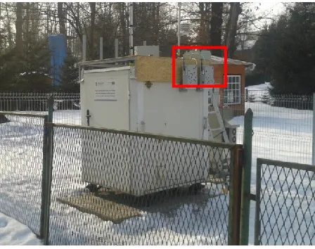
research was conducted at the measuring station of the National Reference and Calibration Laboratory of the Chief Inspectorate of Environmental Protection from February 15th to June 15th, 2017. Research was carried out in the town of Rabka-Zdrój. In order to conduct comparative measurements, two devices (UR1 and UR2) were placed at the reference station – Fig. 1. For comparison with the reference device, 24-hour PM10 concentrations were used because such data was available for the reference station.
Fig. 1. Measuring devices at the reference station in Rabka-Zdrój.
After almost 5 months of comparative measurements, the correlation of the used low-cost sensors was analyzed in relation to the reference device. The results are shown in Table 1. Some other details are also presented in [6, 7].
Table 1. Statistical parameters of results from comparative measurements of two devices in Rabka-Zdrój.
Parameter UR1 UR2
Pearson's correlation coefficient r 0.946 0.912
Mean error (ME) [g/m3] 14.180 10.910
Mean Percentage Error (MPE) [%] 44.720 34.510 Mean Absolute Error (MAE)
[g/m3] 14.860 12.290
Mean Absolute Percentage Error
(MAPE) [%] 46.970 39.240
A large set of comparative data and high correlation with the reference device made it possible to determine the correction function. The polynomial correlation of grade 2 was used as the one for which the obtained convergence was the best in relation to the results of measurements from the reference device (among linear, exponential, logarithmic, polynomial, power correlation). The dependency obtained in this way is as follows:
P’ = -0.0007P2 + 0.674P + 3.35 (1)
where :
P – measured PM10 concentration,
3 Results
[image:4.482.56.425.203.334.2]In order to verify the effectiveness of the correction function, at the end of January 2018 two other measuring devices were placed in Nowy Sącz near the reference station belonging to RIEP. The results of measurements from February and March 2018 are presented below. For comparison, the average 24-hour PM10 concentrations from the RIEP station and measured by two devices equipped with low-cost sensors from the same manufacturer (U1 and U2) were taken into account. Basic statistical parameters calculated from the results of measurements from both low-cost sensors are presented in Tables 2-3. Table 2. Statistical parameters of 24-hour PM10 concentrations in relation to concentrations measured
in the RIEP station – February 2018.
Parameter U1 without correction correction U1 with U2 without correction correction U2 with
Pearson's correlation
coefficient r 0,975 0,973 0,979 0,976
Mean error (ME) [g/m3] 39,210 -3,660 45,920 -0,080 Mean Percentage Error (MPE)
[%] 47,230 -7,050 59,050 -0,040
Mean Absolute Error (MAE)
[g/m3] 40,350 6,830 45,920 5,20
Mean Absolute Percentage
Error (MAPE) [%] 50,330 12,010 59,050 8,460
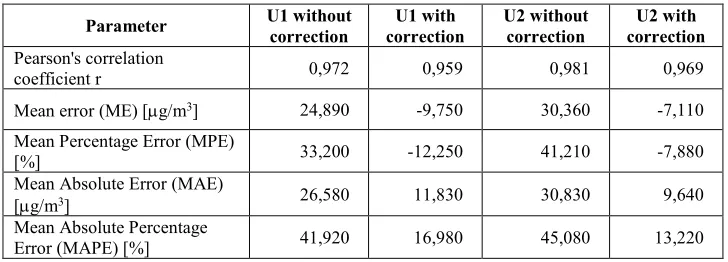
Table 3. Statistical parameters of 24-hour PM10 concentrations in relation to concentrations measured in the RIEP station – March 2018.
Parameter U1 without correction correction U1 with U2 without correction correction U2 with
Pearson's correlation
coefficient r 0,972 0,959 0,981 0,969
Mean error (ME) [g/m3] 24,890 -9,750 30,360 -7,110 Mean Percentage Error (MPE)
[%] 33,200 -12,250 41,210 -7,880
Mean Absolute Error (MAE)
[g/m3] 26,580 11,830 30,830 9,640
Mean Absolute Percentage
Error (MAPE) [%] 41,920 16,980 45,080 13,220
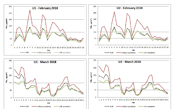
[image:4.482.60.424.365.496.2]Fig. 2. The variability of 24-hour PM10 concentrations from sensors U1 and U2 (without and with the correction function applied) and from the reference station for particular months.
After applying the correction function, determined based on the previous results, a significant improvement in measurement values from both low-cost sensors in relation to the reference station was obtained. Correlation coefficients were still at a very high level, while the greatest improvement was observed in the case of percentage errors and differences in absolute values. In February, in the case of U2 sensor, the average error and the average percentage error were even close to zero. The values of absolute errors have also significantly improved. In February, with an initial overestimation of about 40 g/m3, after correction, the error was lower than 7 g/m3. The improvement for both sensors took place also in March.
In the case of absolute percentage errors in February, there was a drop from 50-60% to 8-11%, while in March from 40-45% to about 13-16%. There was also a significant reduction in overestimations in days with high PM10 concentrations (7, 12 and 13 February), which is presented in Fig. 2. The achievement of the desired effect of the correction function was undoubtedly due to the fact that it was determined on the basis of a comprehensive data set, taking into account measurements carried out at different times of the year and under different atmospheric conditions.
measurements, while for overestimations from the first days of March, unfortunately, caused quite a large undervaluation. Such low temperatures were not observed during comparative measurements in Rabka-Zdrój, therefore, they were not taken into account when determining the corrective function. It also shows that the designated correction function works well under the conditions in which the set of comparative data was created. However, for the conditions that occurred during the initial comparative measurements, the obtained correction fit was quite good.
4 Conclusions
It should be noticed that in the analyzed cases the application of the correction function brought a significant improvement of measurements quality (as for low-cost sensors). On the basis of currently conducted comparative measurements in Nowy Sącz, it is planned to develop a new, improved correction function taking into account the results from both places. Taking into account additional meteorological parameters, such as relative humidity and temperature, may bring even better improvement in the matching of the measurement results coming from low-costs devices in relation to the results from the reference station. The cost of an additional measuring instrument to measure temperature and relative humidity is very small, and therefore cost-effective from the perspective of the quality of the complete device. The sensor itself is very small, which does not disqualify it for use even in a small portable measuring device.
References
1. R. Williams, V. Kilaru, E. Snyder, A. Kaufman, T. Dye, A. Rutter, A. Russell, H. Hafner, Air Sensor Guidebook; Technical report, United States Environmental Protection Agency (2004)
2. J. Shi, F. Chen, Y. Cai, S. Fan, J. Cai, R. Chen, Z. Zhao, PLoS ONE 12(11), e0185700 (2017)
3. B. Mijling, Q. Jiang, D. Jonge, S. Bocconi, Atmos. Meas. Tech., 11, 1297–1312 (2018)
4. L. Crilley, M. Shaw, R. Pound, L. Kramer, R. Price, S. Young, A. Lewis, F. Pope, Atmos. Meas. Tech., 11, 709–720 (2018)
5. Ch. Lin, N. Masey, H. Wu, M. Jackson, D. Carruthers, S. Reis, R. Doherty, I. Beverland, M. Heal, Atmosphere, 8, 231 (2017)
6. M. Rogulski, Energy Procedia, 128, 437-444 (2017)