Development of energy selective techniques in x ray computed tomography

techniques in X-ray computed

tomography

Mahsa Paziresh

A thesis submitted for the degree of

DOCTORATE OF PHILOSOPHY

The Australian National University

between them and me. It was heart-warming to daily have contact and feel their love and encouragement. I dedicate this dissertation to them. I also would like to express my heart-felt gratitude to the rest of my family- Maryam Paziresh, Kaivan

I would like to acknowledge the support of the chair of my supervisory panel, Prof Adrian Sheppard, and my two PhD advisors, Dr Andrew Kingston and Dr Glenn Myers. I am particularly grateful to Prof Adrian Sheppard for numerous dis-cussions on my research and lectures on related topics that helped me improve my thesis. Also, I shared an office with Dr Andrew Kingston and I appreciate the long discussions we had on the technical details of my work. I am also thankful to Dr Wilfred Fullagar and Dr Shane Latham for their insightful comments. I thank Dr Glenn Myers, Dr Wilfred Fullagar, Dr Shane Latham, and Dr Andrew Kingston for carefully reading and commenting on countless revisions of research manuscripts. I have been fortunate to have supervisors who gave me the freedom to explore on my own and, at the same time, the guidance to recover when my steps faltered. I doubt that I will ever be able to convey my appreciation fully, but I owe them my eternal gratitude.

Prof Tim Senden, the head of Research School of the Physics and Engineering, and Prof Adrian Sheppard, the head of the Applied Mathematics Department, have been always there to listen and give advice, despite their busy schedules. I am so very thankful to them for offering a great deal of their time, consistent encourage-ment, practical advice and generous support that provided me with the opportunity to improve my thesis.

Also, I appreciate Clare Idriss of Practical Editing for her assistance with editing my thesis in line with the use of correct grammar and consistent notation in my writ-ings.

A very special thanks goes out to Dr Mathieu Salzmann from National ICT Aus-tralia (NICTA), who offered motivation and encouragement in my PhD studies. He provided me with direction, support and became more of a mentor and friend, than a professor. It was his persistence, understanding and kindness that initially encour-aged me to pursue my studies.

I am also grateful to the following staff at the Research School of Physics and Engineering for their various forms of support during my graduate study: Prof Lan fu, Martina Landsmann, Luidmila Mangos and Karen Nulty.

Finally and most importantly, I would like to express my appreciation for study-ing at the Australian National University (ANU). I am indebted to this university for the great support and the professional guidance through every stage of my graduate studies. I appreciate the financial support I received from the ANU for funding my research discussed in this dissertation with the ANU PhD scholarship and providing me with access to the ANUµCT facility.

“Paziresh M, Kingston A. M, Latham S. J, Fullagar W. K, and Myers G. M. 2016. Tomography of atomic number and density of materials using dual-energy imaging and the Alvarez and Macovski attenuation model. Journal of Applied Physics. 119, 21 (2016), 214901."

“Fullagar W. K, Kingston A. M, Myers G. M, and Paziresh M. 2016. Average quantum energy from measurements of intensity and its noise." In preparation.

“Paziresh M, Kingston A. M, Fullagar W. K, and Myers G. M. 2016. Tomography of atomic number and density of materials using single-energy imaging and statisti-cal variance." In preparation.

“Paziresh M, Kingston A. M, Fullagar W. K, and Myers G. M. 2016. X-ray Beam hardening correction using single-energy imaging and statistical variance." In prepa-ration.

“Paziresh M, Latham S. J, and Kingston A, Fullagar W. K, and Myers G. M. 2016. Performance assessment of two simplified forms of Alvarez and Macovski models in comparison with the full model." In preparation.

“Paziresh M, Kingston A. M, Myers G. M, and Latham S. J, and Adrian Sheppard. 2016. Assessment of several linearisation models for X-ray beam hardening correc-tion of cylindrical specimens. In preparacorrec-tion."

“Paziresh M, Recur B, Myers G. M, and Kingston A. K. 2015. Dual-energy ma-terial discrimination. Proceedings of the 2nd International Conference on Tomography of Materials and Structures (ICTMS 2015). PP. 97-98."

“Recur B, Paziresh M, Myers G. M, Latham S. J, Sheppard A. 2014. Dual-energy iterative reconstruction for material characterisation. Proceedings of SPIE Optical En-gineering + Applications. PP. 9212-921213-9."

“Recur B, Paziresh M, Myers G. M, and Kingston A, Latham S and Sheppard A. 2016. Tomographic reconstruction of material characterization. FEI company. WO/2016/028654".

X-ray micro computed tomography (µCT) has emerged as a powerful tool in petroleum industry for non-destructive 3D imaging of rock samples that offers micron-scale resolution images of the distribution of the rock specimens. µCT enables the modelling of the geomechanical and transport properties [Golab et al., 2010] of rocks. µCT obtains the radiographic projections of a sample at different angles and uses a mathematical procedure to reconstruct a 3D tomogram of the sample’s X-ray attenu-ation coefficients. Attenuattenu-ation coefficient is a quantity that describes to what extent the X-ray beam is reduced as it passes through a sample. Through my thesis, the aim was to investigate and improve the two main issue from whichµCT suffers:

1) µCT X-ray sources typically emit polychromatic X-rays. When an X-ray beam passes through a sample, the low energy photons (or soft X-rays) are attenuated more readily, leaving a beam consisting of more high energy photons (or hard X-rays), i.e., “X-ray beam hardening” (BH). Therefore the recorded attenuation, given by the loga-rithm of the ratio of the attenuated and incoming X-ray beam, i.e., Beer-Lambert law, is no longer a linear function of material thickness. If this nonlinear effect is not com-pensated for, the tomograms will be corrupted by severe edge, “cupping artefact" and “streaks" between dense materials. Apart from these visual aspects, quantitative problems may arise, thus, these artefacts make subsequent tomogram segmentation and analysis difficult.

2)µCT produce micro resolution structural images of a sample but not the com-positional information. AlthoughµCT can discriminate sample materials with totally different attenuation coefficients, there are samples such as rocks that include mate-rials with similar attenuation coefficients at one energy spectra. In that case, the attenuation coefficients of materials in an altered energy spectra may be different.

This thesis contributes in addressing the above mentioned fundamental issues in µCT by providing “energy selective techniques" in: 1) BH correction and 2) material characterisation. These methods consider the energy dependency of attenuation co-efficients and polychromatic nature of X-rays. The structure of thesis is as follows:

further and use the energy dependency ofµCT as a benefit to characterise the sample materials.

Chapter 2 presents an overview of the physics of BH and the existing correction methods with their advantages and disadvantages, followed by a brief review of the material characterisation methods and the recent advances in this field.

Chapter 3 assess the accuracy of five different linearisation BH correction mod-els including polynomial, bimodal, power law, cubic spline and linear spline using the samples that have been imaged at the ANU µCT facility by measuring the BH curves directly from the projection data in a manner similar to that obtained by imag-ing wedge phantoms, and remappimag-ing the inverse of the models to data. The cubic spline, power law, and polynomial models were found to have the lowest root mean square errors, which for all samples were on average 6.36×10−1%, 6.24×10−1%, and 6.41×10−1% respectively. The number of parameters to be estimated in power law is the lowest, therefore, considering the small differences in comparing the errors of power law, polynomial and cubic spline models, the power law is a good, simple model for the ANUµCT system.

Chapter 4 is based on a published conference proceeding paper in the “ Inter-national Conference of Tomography of Materials and Structures (ICTMS2013)" [Paziresh et al., 2013] which applies the power law linearisation BH correction method of chap-ter 3 to correct the BH artefacts of specimens composed of nested-cylinders, e.g., a rock core within a container. The amount of BH varies depending on the material composition of the specimen and the incident X-ray spectrum. BH can be corrected for each material provided a BH curve is known. The BH curves were obtained by assuming a uniform material for each cylinder. This chapter describes how to deter-mine the centre and radius of each cylinder, generate their BH curves and fit them with a power law model to linearise the total projection data. The BH artefacts are significantly reduced in the tomographic reconstructions resulting from these cor-rected projections.

2010; Kaewkhao et al., 2008]. The model requires calibration and has several limita-tions, i.e., the model doesn’t account for K-edges and there’s no agreed value upon some parameters of the model. I calibrated and used the full model to estimate the ρ andZof sample materials. This chapter describes the tomographic reconstruction of ρ and Z maps of mineralogical samples using the AMTI model. The full model requires precise knowledge of the X-ray energy spectra and calibration of PE and CS constants and exponents of atomic number and energy that I estimated based on fits to simulations and calibration measurements. The estimated ρ andZ images of the samples used in this chapter yield average relative errors of 2.62% and 1.19% and maximum relative errors of 2.64% and 7.85%, respectively. Furthermore, I demon-strate that the method accounts for the BH effect in ρ and Z reconstructions to a significant extent.

Chapter 6 implements two simplified forms of the full model of chapter 5: 1) Al-varez and Macovski polynomial (AMP) model [AlAl-varez and Macovski, 1976], AlAl-varez and Macovski presented the full model but used a polynomial simplified form of it to estimateρandZof materials; and 2) Siddiqui and Khamees (SK) model [Siddiqui et al., 2004] that simplified the attenuation model, by assuming two monochromatic radiation. The AMP model, similar to the AMTI model performs the analyses on the projections, but unlike the AMTI doesn’t account for the energy dependency of the attenuation coefficients and X-rays, thus, the image captured in the PE energy range and, so the resultant Z image, includes BH artefacts. The results from the SK method are more stable since analysis is performed directly on the tomogram. How-ever, since BH correction must be performed on the low-energy reconstructions, this hinders any accurate estimation of ρ and Z. The results for the AMTI model are, on average for the reference materials used, more accurate than both the AMP and SK models for both atomic number and density estimation. That is, more accurate for atomic number estimation by 7.81% and 15.9%, and more accurate for density estimation by 4.73% and 13.00%, than the AMP and SK models, respectively.

Chapter 7 presents a method to estimate the properties of sample materials from measurements of transmitted intensity and its statistical variance (TIV model). The method only requires single-energy imaging, i.e.; eliminates the requirement of dual-energy. The registered intensity on the detector is proportional to a form of “average" energy of detected quanta of X-ray spectra. The statistical variance of images is then modelled as a Poisson distribution. The variance images can serve the same purpose as the higher energy information required in dual-energy imaging. This chapter ex-amines the effect of energy and spectra on Z and ρ calculations. More registered photons and a higher number of collected radiographs provide less relative error in Zand ρ estimations. The proposed model yields average estimatedρ and Z values 4.29% and 2.47% error. The model correct the BH artefacts reasonably well.

Acknowledgments vii

Publications ix

Patents xi

Abstract xiii

1 X-ray micro Computed-Tomography 1

1.1 Introduction . . . 1

1.2 X-ray micro computed-tomography (µCT) . . . 2

1.2.1 Comparison of clinical CT andµCT . . . 2

1.2.2 X-rays . . . 3

1.2.3 X-ray source . . . 3

1.2.3.1 X-ray micro-focus tube . . . 6

1.2.4 X-ray detector . . . 8

1.2.4.1 Scintillator . . . 8

1.2.5 Basic interaction of X-rays with matter . . . 9

1.2.5.1 Photoelectric absorption . . . 9

1.2.5.2 Compton scattering . . . 9

1.2.5.3 Rayleigh scattering . . . 10

1.2.6 Attenuation of X-rays . . . 11

1.2.6.1 Linearisation . . . 13

1.2.7 Image reconstruction . . . 14

1.2.7.1 Line integrals and projections . . . 14

1.2.7.2 The Fourier slice theorem . . . 17

1.2.7.3 The filtered back-projection (FBP) . . . 20

1.2.7.4 Fan beam . . . 24

1.2.7.5 Cone beam . . . 26

1.3 Conclusion . . . 26

2 Energy selective techniques 29 2.1 Introduction . . . 29

2.2 Beam hardening (BH) artefacts and correction techniques in CT . . . 30

2.2.1 Hardware filtering . . . 34

2.2.2.1 Linearisation BH correction by minimising re-projection

distance . . . 36

2.2.2.2 Linearisation iterative expert-guided BH correction for heterogeneous specimens . . . 38

2.2.3 Post-reconstruction iterative BH software correction methods . . 40

2.2.3.1 Post-reconstruction iterative, reference-less BH correc-tion method . . . 40

2.2.3.2 Post-recontruction iterative BH correction based on a physical model . . . 43

2.3 Material characterisation in CT . . . 45

2.3.1 Correction on Siddiqui and Khamees (SK) method . . . 46

2.3.2 Source-weighting method . . . 49

2.4 Conclusion . . . 51

3 Assessment of several linearisation X-ray beam hardening correction meth-ods 53 3.1 Introduction . . . 53

3.2 Measuring beam hardening curves . . . 55

3.2.1 Wedge and cylinder phantoms . . . 55

3.2.2 Beam hardening curves of common materials at the ANUµCT facility . . . 56

3.3 Fitting BH curve models and performing BH correction . . . 61

3.3.1 Polynomial model . . . 63

3.3.2 Bimodal energy model . . . 65

3.3.3 Power law model . . . 67

3.3.4 Cubic spline model . . . 69

3.3.5 Linear spline model . . . 70

3.4 Performance assessment of the applied linearisation BH correction mod-els . . . 72

3.5 Conclusion . . . 73

4 Beam hardening correction of concentric cylindrical specimens using power law model 75 4.1 Introduction . . . 75

4.2 Fitting the cylinder (or circles) . . . 76

4.3 Fitting material attenuation . . . 77

4.4 Fitting the beam hardening correction model . . . 77

4.5 Applying the beam hardening correction . . . 78

4.5.1 Single cylinder . . . 78

4.5.2 Nested-cylinders . . . 78

5 Material characterisation using dual-energy imaging and the AM

attenua-tion model 85

5.1 Introduction . . . 85

5.2 Alvarez and Macovski attenuation coefficient (AMAC) and transmit-ted intensity (AMTI) models . . . 88

5.3 Modelling the physics of X-ray energy spectrum [Sε(E)] . . . 90

5.3.1 Measuring the X-ray energy spectrum . . . 93

5.3.1.1 Correction of the partial registry of the measured X-ray spectra on the detector . . . 93

5.3.2 Correction of the characteristic peaks of the simulated X-ray spectra . . . 95

5.3.3 X-ray dual-spectra . . . 96

5.4 Simulation: Validating and calibrating the model . . . 97

5.4.1 AMAC model calibration using NIST data . . . 98

5.4.2 AMTI model calibration using simulated cylinder images . . . . 101

5.4.3 Testing the AMTI model calibration using the real cylinder im-ages . . . 105

5.5 Experimental analysis . . . 108

5.5.1 Material discrimination of rock using AMTI model . . . 110

5.5.2 Beam hardening correction in AMTI model . . . 113

5.6 Conclusion . . . 115

6 Assessment of the full AM model in comparison with two simplified forms117 6.1 Introduction . . . 117

6.2 Alvarez and Macovski Polynomial (AMP) transmitted intensity model . 118 6.2.1 The AMP model calibration using the real cylinder images . . . 118

6.2.2 Material discrimination of rock using AMP model . . . 122

6.3 Siddiqui and Khamees (SK) attenuation model . . . 126

6.3.1 The SK model calibration using the real cylinder images . . . 128

6.3.2 Material discrimination of rock using SK model . . . 129

6.4 Assessing the atomic number and density estimations of AMP and SK models in comparison with the results of the full AMTI model (from chapter 5) . . . 131

6.5 Conclusion . . . 133

7 Material characterisation using single-energy imaging and statistical vari-ance 135 7.1 Introduction . . . 135

7.2 The correlation of Transmitted Intensity and Variance . . . 137

7.3 Transmitted Intensity and Variance (TIV) model for material character-isation . . . 138

7.5.1 Accuracy assessment of TIV model for different X-ray energy spectra . . . 147 7.5.2 Accuracy assessment of TIV model for detected X-ray photons . 148 7.6 Conclusion . . . 149 8 Beam hardening correction using single-energy imaging and statistical

vari-ance 151

8.1 Introduction . . . 151 8.2 The performance of energy in beam hardening correction (BH) methods 153 8.3 Transmitted intensity and statistical variance (TIV) model for BH

cor-rection . . . 154 8.4 Simplified Transmitted Intensity and Variance (STIV) model for BH

correction . . . 157 8.5 Conclusion . . . 158

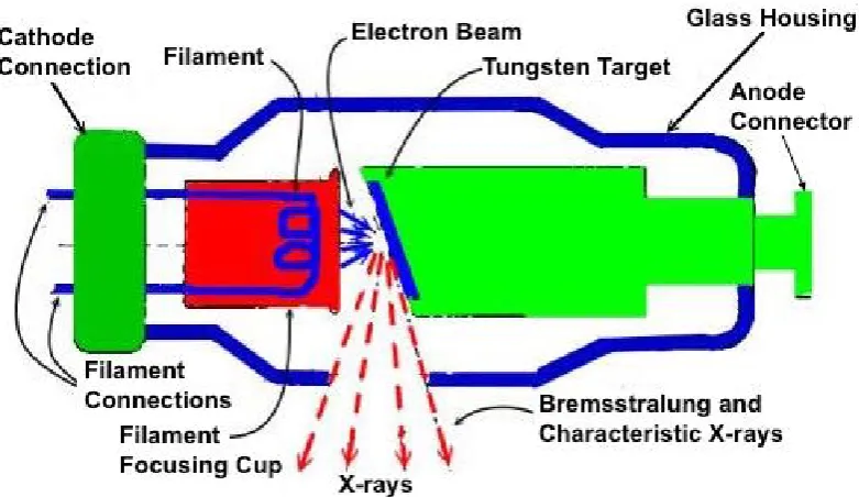
1.1 Schematic overview of an X-ray source tube and its component (http://doctorspiller.com/Dental%20radiologyx-ray_characteristics.html). . . 4

1.2 Schematic overview of: a) characteristic and b) Bremsstrahlung X-ray productions [Mohamed, 2013]. . . 5 1.3 X-ray spectrum of a tungsten source for a maximum tube voltage of

100 keV, filtered by 0.1mm Cu measured using Amptek CdTe spectrum analyser. . . 6 1.4 Schematic overview of an micro-focus X-ray source tube and its

com-ponent (http://www.yxlon.com/Technology). . . 7 1.5 The fine focus imaging geometry. . . 7 1.6 Mass Attenuation Coefficient for a soft tissue [Ajaja, 2010]. . . 9 1.7 For X-ray imaging in the energy ranges used in medical CT and µCT

two interactions are important: (a) the photoelectric absorption and (b) the Compton scattering (http://www.studyblue.com). . . 11 1.8 Coordinate transformation of sampleµ(x,y)to the projectionPθ(t)[Kak

and Slaney, 1988]. . . 15 1.9 A parallel projection is formed by measuring set of parallel rays of

different angles [Kak and Slaney, 1988]. . . 16 1.10 The Fourier slice theorem relates the Fourier transform of a

projec-tion to the Fourier transform of a sample along a radial line [Kak and Slaney, 1988]. . . 18 1.11 Collecting projections of the sample at a number of angles provides

es-timation of the Fourier transform of the sample along radial lines [Kak and Slaney, 1988]. . . 20 1.12 Schematic of 1D projection of a sample at three different angles and

the corresponding reconstruction from the obtained projection data (http://bruker-microct.com/home.htm). . . 21 1.13 The dependency of the quality of the reconstruction image of a point

sample on the available projection data from different angles (http://bruker-microct.com/home.htm). . . 21 1.14 The blur around the reconstructed image after back-projection

recon-struction and the correction of the blur using a filter (http://bruker-microct.com/home.htm). . . 22 1.15 Schematic view of the projection filter,h(t), in the spatial domain [Kak

1.16 A fan beam projection is collected if all the rays meet in one loca-tion [Kak and Slaney, 1988]. . . 25 2.1 Attenuation of a) Silicon and b) Platinum as a function of photon

En-ergy (http://physics.nist.gov/PhysRefData/XrayMassCoef/tab4.html). These plots are presented to show that the nonlinear trend of the at-tenuation coefficients result in the nonlinearity of the beam hardening artefacts (see Eqn. 1.2). Plots of the attenuation for the energy range of imaging in this thesis, [1, 120] keV, are presented in figure 5.7 for several samples used in the experiments. . . 31 2.2 Effect of beam hardening on reduction of spectra’s photon counts as

the beam is passing through the aluminium filters with thickness of 0.25, 0.5, 1, 2, 4, 6 mm shown subsequently in green, blue, red, purple, yellow and black colours. The spectra is recorded using Amptek CdTe spectrum analyser. . . 32 2.3 Illustration of BH effect; (i) a sample made of PMMA and aluminium,

(ii) reconstruction including BH artefacts, (iii) BH corrected reconstruc-tion and (iv) a line through the reconstrucreconstruc-tions [Van Gompel et al., 2011]. 33 2.4 Hardware Filtering. The spectra imaged at 60 keV with 0.25 mm Al

filter and100 keV with 0.25 mm Cu filter, using Amptek CdTe spectrum analyser. . . 34 2.5 Flowchart of the linearisation BH correction by minimising re-projection

distance (Section 2.2.2.1) [Kingston et al., 2012]. . . 37 2.6 Flowchart of the iterative expert-guided BH correction method

(Sec-tion 2.2.2.2) [Ketcham and Hanna, 2014]. . . 39 2.7 Flowchart of the iterative reference-less BH correction (Section 2.2.3.1) [Krumm

et al., 2008]. . . 41 2.8 (a) shows the polychromatic and (b) the monochromatic

approxima-tion of the point cloudpropagaapproxima-tion path length versus ray sum plot of a two-material specimen, by a two-dimensional plane and surface with 400 nodes. Black dots indicate computed attenuation values [Krumm et al., 2008]. . . 42 2.9 Flowchart of the iterative physical energy distribution BH correction

(Section 2.2.3.2) [Van Gompel et al., 2011]. . . 44 2.10 Flowchart of estimation of the corrections to be applied on the SK

method; withebeing the relative error andδ being the absolute error (Section 2.3.1) [Derzhi, 2012]. . . 47 2.11 Flowchart of applying the corrections of Fig. 2.10 on the SK method

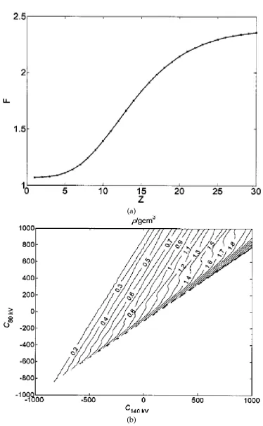
(Section 2.3.1) [Derzhi, 2012]. . . 48 2.12 Plots of the numerical results of Z and ρ projections: a) shows a

function, F(Z) = µ1

µ2, and b) shows ρ(µ1,µ2) for recorded images at

80 and 140 keV (µ1 and µ2 are normalised to CT values C; where

C=1000×µ−µwater

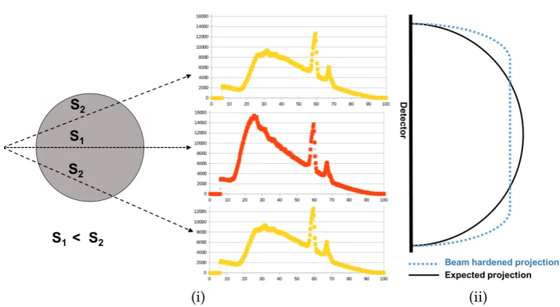
3.1 Illustration of the BH (i) the quantitative measurement of source with different filters corresponding to the thickness of the shown sample (S1 = 0.5mm and S2 = 2mm Al filter), and (ii) schematics drawing of

beam hardened and the ideal projection. . . 56 3.2 Schematic of plotting the BH curve, i.e., the intensity of the projection

versus the path length of X-ray (s) for a cylindrical sample. . . 58 3.3 The attenuation of the X-ray spectra using different filters or container,

as the beam is passing through the sample. This plots are quantita-tive measurement of source with different filters corresponding to the thickness of the shown sample: (i) S1 = 0.5mm and S2 = 0.5mm Al

filter, (ii) S1 = 0.5mm Al and S2 = 1mm Al filter, (iii) S1 = 0.5mm Al

andS2 =2mm Al filter. . . 59

3.4 BH curve of (i) NaI, (ii) CsI, (iii) CsCl, (iv) 100 per BrC, (v) BrC8 in oil,

and (vi) ICxwith different salinities. . . 60

3.5 A cross-sectional reconstructed uncorrected image of 2M CsI in cylin-drical container. . . 61 3.6 Flowchart of linearisation BH correction. The BH curve of samples

can be obtained having prior knowledge of sample shape, i.e., wedge or cylindrical specimens of uniform composition, i.e., homogeneous samples (see section 3.2.1 and Fig. 3.1 and 3.2). . . 62 3.7 Plot of the uncorrected (main) data, polynomial of order eight fit and

the corrected (linearised) data . . . 63 3.8 (i) A cross-sectional reconstruction of 2M CsI in a cylindrical container

corrected by applying the polynomial model of order (a-four, b-six, c-eight), (ii) profile through the centre of the uncorrected (blue line) and corrected (red line) images. . . 64 3.9 Plot of the uncorrected (main) data, bimodal fit and the corrected

(lin-earised) data . . . 66 3.10 (i) A cross-sectional reconstruction of 2M CsI in a cylindrical container

corrected by applying the bimodal model, (ii) profile through the cen-tre of the uncorrected image (blue line) and the corrected image (red line) image. . . 66 3.11 Measured X-ray BH curves at our facility [Paziresh et al., 2013] . . . 67 3.12 Plot of the uncorrected (main) data, power law fit and the corrected

(linearised) data . . . 68 3.13 (i) A cross-sectional reconstruction of 2M CsI in a cylindrical container

corrected by applying the power law model, (ii) profile through the centre of the uncorrected image (blue line) and the corrected image (red line) image. . . 68 3.14 Plot of the uncorrected (main) data, spline fit and the corrected

3.15 (i) A cross-sectional reconstruction of 2M CsI in a cylindrical container corrected by applying the spline model, (ii) profile through the centre of the uncorrected image (blue line) and the corrected image (red line) image. . . 70 3.16 (i) A cross-sectional reconstruction of 2M CsI in a cylindrical

con-tainer corrected by applying the linear spline model with (a-2_lines, b-3_lines), and (ii) profile through the centre of the uncorrected image (blue line) and the corrected image (red line) image. . . 71 3.17 The average RMS error of corrected images compared with uniform disc. 72 4.1 Horizontal slices through two single cylinder specimens (a) . (i)

re-constructions with beam-hardening artefacts, (ii) rere-constructions after correction, and (iii) profile through the centre of images as indicated by dashed lines . . . 79 4.2 Horizontal slices through two single cylinder specimens (b). (i)

re-constructions with beam-hardening artefacts, (ii) rere-constructions after correction, and (iii) profile through the centre of images as indicated by dashed lines . . . 80 4.3 Flowchart of the BH correction of nested-cylinders. . . 81 4.4 A horizontal slice through a three cylinder specimen including the

rock, fluid and the holder. (i) reconstructed using measured attenu-ation, (ii) reconstructed using corrected attenuattenu-ation, and (iii) profile through the centre of images as indicated by dashed lines . . . 82 5.1 Flowchart of the Modelling the physics of X-ray energy spectrum [Sε(E)],

withε being the energy label. . . 91 5.2 Simulated spectrum at 100 maximum energy; modified to match that

seen for our experimental protocol, meaning that the spectrum is mod-ified to be as measured by the detector with CsI scintillator. The plot shows a jump at 33.169 keV that relates to the K-edge of Iodine. . . 92

5.3 Attenuation of CsI as a function of photon Energy (http://physics.nist.gov/PhysRefData/XrayMassCoef/tab4.html). 93 5.4 Plot of partial register correction using the stripping algorithm for a)

80 (blue line [Redus et al., 2009]), b) 60, c) 100 and d) 120 keV spectrum measured using the Amptek spectrum analyser. The yellow line is the measured partial registry corresponding to the four terms fj(E− Ej)Nd(E)in Eqn. 5.7 . . . 95 5.5 Plot of the partial registry corrected measured spectrum fitted to

sim-ulated spectrum to match the XRFs amplitude for : a) 80 ([Redus et al., 2009]) , b) 60, c) 100 and d) 120 keV . . . 96 5.6 Simulated dual-energy spectra at 60 (red line) and 120 keV (blue line)

5.7 Plot of ln(µ) versus (E = [1, 120]keV) of NIST data (red line) and AMAC model (blue dashed line) fits applying the the estimated K1,

K2, m and n constants in section 5.4.1 for a) glass, b) acrylic, c)

tita-nium and d) marble. . . 100 5.8 Flowchart of the AMAC model calibration (Section 5.4.1). . . 101 5.9 A line through a simulated projection cylinder and the AMTI model

fit: at 60 keV (red line and dashed cyan line) and 120 keV (blue and dashed green line) maximum energies for a)glass and b) marble . . . . 102 5.10 Flowchart of the AMTI model calibration andρ andZ estimation,

us-ing simulated projections of cylinders of 7 reference materials (Sec-tion 5.4.2), with ε being the energy label and pre-processing step ex-plained in section 5.5. P =R

L

p(s,E)andC =R L

c(s,E)from Eq. 5.3. . . 104 5.11 A line through an imaged projection cylinder and the AMTI model

fit: at 60 keV (red line and dashed cyan line) and 120 keV (blue and dashed green line) maximum energies for a)glass and b) marble. . . 106 5.12 Flowchart of the AMTI model calibration andρ andZ estimation,

us-ing real intensity images of cylinders of 7 reference materials (Sec-tion 5.4.3), with ε being the energy label and pre-processing step ex-plained in section 5.5. P =R

L

p(s,E)andC =R

L

c(s,E)from Eq. 5.3. . . 107 5.13 Flowchart of ρ and Z estimation using real intensity images of

cylin-ders of rocks and the calibrated AMTI model (Section 5.5), with ε be-ing the energy label and pre-processbe-ing step explained in section 5.5. P =R

L

p(s,E)andC =R

L

c(s,E)from Eq. 5.3. . . 109 5.14 a-i) reconstructed slice of Berea sandstone atEmax

ε =60keV, b-i)

recon-structed slice Berea sandstone at E_εmax = 120keV, a-ii) reconstructed slice of the estimated Z using the AMTI model 5.5 and b-ii) recon-structed slice of the estimated ρ using the AMTI model. The cupping artefacts are evident around the edges in a-i, while a-ii and b-ii don’t have the BH artefacts. The image contrast in enhanced to illustrate the existence of the cupping artefact in a-i and no visible BH in b-i, however the a-ii and b-ii images shows the original grey scales of the images. . . 111 5.15 a-i) reconstructed slice of the carbonate masked Z, b-i) reconstructed

6.1 Flowchart of the AMP model calibration andρandZestimation, using real intensity images of cylinders of 7 reference materials (Section 6.2), with ε being the energy label and pre-processing step explained in section 5.5. P = R

L

p(s,E)andC =R

L

c(s,E)from Eq. 5.3. . . 121 6.2 a-i) reconstructed slice of the estimated Z of Berea sandstone, using

the AMP model ( 6.1), b-i) reconstructed slice of the estimated ρ of Berea sandstone using the AMP model, a-ii) the plot of fitted Gaussian to the histogram of masked Z, and b-ii) the plot of fitted Gaussian to the histogram of maskedρ(see Fig. 5.14a-ii and b-ii for reconstruction slice of Berea sandstone imaged atEmax_{=60 and 120 keV) . . . 124}

6.3 a-i) reconstructed slice of the estimated Z of the carbonate, using the AMP model 6.1, b-i) reconstructed slice of the estimated ρ using the AMP model, a-ii) the plot of fitted Gaussian to the histogram of masked Z, and b-ii) the plot of fitted Gaussian to the histogram of masked ρ (see Fig. 5.15a-i and b-i for more details about masked Z andρ) . . . 125 6.4 Flowchart of the SK model calibration and ρ and Z estimation, using

reconstructed images of cylinders of reference materials (Section 6.3). One can choose to have different number of reference materials,ω. We have chosen 7 reference materials, commonly used at the AnuµCT fa-cility, for the calibration of the models in chapter 5 to 8. This materials are over a range of atomic number and density. . . 127 6.5 a-i) reconstructed slice the estimated Z of the Berea sandstone, using

the SK model 6.3, b-i) reconstructed slice of the estimated ρ of the Berea sandstone using the SK model, a-ii) the plot of fitted Gaussian to the histogram of masked Z and b-ii) the plot of fitted Gaussian to the histogram of maskedρ(see Fig. 5.14a-ii and b-ii for reconstruction slice of Berea sandstone images atEmax_{=60 and 120 keV) . . . 130}

6.6 a-i) reconstructed slice of the estimated Z of the carbonate, using the SK model 6.3, b-i) reconstructed slice of the estimated ρ of the car-bonate using the SK model, a-ii) the plot of fitted Gaussian to the histogram of masked Zand b-ii) the plot of fitted Gaussian to the his-togram of masked ρ (see Fig. 5.15a-i and b-i for more details about masked Z andρ) . . . 131 7.1 Simulated energy spectra at 100 keV maximum energy with 0.5 mm

aluminium filter (red line) and the spectrum including higher mean energy (blue line); modified to match that seen for our experimental protocol. . . 139 7.2 A line through a simulated projection cylinder and the TIV model fit:

7.3 Flowchart of the TIV model calibration andρand Zestimation, using simulated projections of cylinders of 7 reference materials (Section 7.4), with ε being the energy label. P = R

L

p(s,E) and C = R

L

c(s,E) from Eq. 5.3. . . 143 7.4 A line through a simulated projection and the TIV model fit of the

cylinders of a) glass and b) carbon imaged at 100 keV. . . 145 7.5 Flowchart of the TIV model calibration andρand Zestimation, using

simulated projections of cylinders of 7 reference materials (Section 7.5), with ε being the energy label. P = R

L

p(s,E) and C = R

L

c(s,E) from Eq. 5.3. . . 146 8.1 Simulated energy spectra at 40 keV maximum energy with no filter

(red line) and the spectrum including higher mean energy (blue line); modified to match that seen for our experimental protocol. . . 154 8.2 A line through reconstruction of glass, showing the average intensity

captured at 40 keV (blue line), statistical variance (green line) and the applied TIV BH correction in section 8.3 (red line). The reconstruction of this study are from a single radiograph. Since the same noise copied to the all projection angles, the line profile of the reconstructed image also include ring artefacts. . . 155 8.3 Flowchart of the modified TIV model for beam hardening correction,

using simulated projections of cylinders of 7 reference materials (Sec-tion 8.3), withεbeing the energy label. P =R

L

p(s,E)andC= R L

c(s,E) from Eq. 5.3. . . 156 8.4 A line through reconstruction of marble, showing the average intensity

5.1 Relative error between NIST attenuation coefficient and AMAC model for reference materials using AMAC model (Section 5.4.1). . . 100 5.2 Estimated effective atomic number and bulk density of reference

ma-terials using AMTI model (Section 5.4.2 and 5.4.3). . . 106 5.3 Estimated effective atomic number and bulk density of rocks using

AMTI model (Section 5.5.1). . . 110 6.1 Estimated calibration parameters for AMP model (Eqn. 6.1). . . 119 6.2 Estimated effective atomic number and bulk density of reference

ma-terials using AMP model (Eqn. 6.1). . . 120 6.3 Effective atomic number and bulk density of rocks using AMP model. . 123 6.4 Estimated calibration parameters for SK model (Eqn. 6.4). . . 128 6.5 Estimated effective atomic number and bulk density of reference

ma-terials using SK model (Eqn. 6.3). . . 129 6.6 Effective atomic number and bulk density of materials . . . 130 7.1 Estimated effective atomic number and bulk density of reference

ma-terials using TIV model (Section 7.4). . . 144 7.2 Estimated relative error of effective atomic number of reference

mate-rials using TIV model for different X-ray spectra (Section 7.5.1). . . 147 7.3 Estimated relative error of the bulk density of reference materials using

TIV model for several X-ray spectra (Section 7.5.1). . . 147 7.4 Average estimated relative error of the ρ and Z of the seven samples

for a) detected photon with 1000 image acquisition, and b) acquisition number with 100,000 detected photon. . . 148 7.5 Estimated effective atomic number and bulk density of reference

X-ray micro Computed-Tomography

1

.

1

Introduction

In 1895, Wilhelm Rontgen [Röntgen, 1896] discovered the X-ray beam while he was experimenting an electric discharge in a vacuum tube in his laboratory. He no-ticed a radiation on a phosphor screen in front of the tube. He positioned different materials in front of the screen to examine which one could block the beam. When he put his hands in front of the screen, he saw a shadowed image of his bones. As such, X-rays were discovered and at the same time radiography was born. Rontegen received the Nobel Prize in 1901 for his discovery [Röntgen, 1896].

A radiograph only provides a two dimensional (2D) projected image (projection) of a three dimensional (3D) sample; where projection is the line integral of X-ray beam attenuation along the direction of X-ray propagation. This 2D projection of 3D sample can help to diagnose a broken bone but, having the information about the depth (3rddimension) could facilitate more precise examination. Tomography solved this limitation by capturing these projected radiographs of the sample at different angles, this way, depth could be taken into account in reconstruction. The word tomography is a combination of two Greek words: “tomos” and “graphos” which respectively mean “slice” and “to draw”.

Micrometer-scale computed-tomography (µCT), like medical computed-tomography, uses X-ray imaging combined with the inverse Radon transform to reconstruct the cross-sections, or the even full 3D view, of a sample without destroying the original specimen. µCT allows quantitative analysis of the thickness or composition of the sample material. The first X-ray µCT system was built by Jim Elliott in the early 1980s [Elliott and Dover, 1982].

X-ray µCT system have a micro-focus source that emits polychromatic X-ray beam. When the X-ray beam is passing through a sample, the X-rays interact with matter and are attenuated. Attenuation coefficient describe the extent to which the X-ray photons are attenuated and is dependent on the applied X-ray energy and the density and atomic number of the sample material.

In this chapter, section 1.2 is a survey of the X-ray µCT systems including X-ray source, detector, production of X-ray spectrum, interaction of X-ray with matter and the energy-dependent attenuation of X-rays. This chapter also includes a summary of a µCT image reconstruction method including measurements of projections, the filtered back-projection reconstruction algorithm and X-ray imaging geometries. This background study lays the foundation for understanding the challenges of energy related issues inµCT and possible solutions.

1

.

2

X-ray micro computed-tomography (

µ

CT)

X-ray computed-tomography (CT) or computerised axial tomography (CAT) use a combinations of several X-ray images at different angles to produce cross-sectional images of a sample. These cross-sectional images provide information about the in-ternal structure of the sample and allow investigation of the specific areas of the sample without cutting into it. Since the introduction of CT in 1970s, the most com-mon applications are found in medicine.

X-ray micro computed-tomography (µCT), like CT, uses X-rays to create cross-sectional images of a sample that can be used to reconstruct a virtual (computerised) 3D model without destroying the original sample. The prefix µ indicates that the pixel sizes of the cross-sections are in the micro-metre range. µCT has found appli-cations both in medical and industrial imaging.

1.2.1 Comparison of clinical CT and µCT

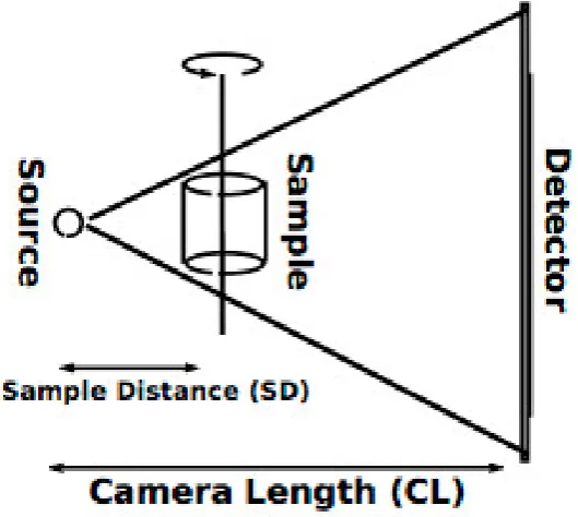
a more stable set-up than clinical CT where the rotating source-detector unit causes vibrations during image acquisition. This supports the ability of a µCT system to produce an enhanced resolution, which is an advantage of this system over clinical CT. Also in µCT, while the sample is rotating, projections can be taken using fan beam (see section 1.2.7.4) or a cone beam geometry (see section 1.2.7.5) along the op-tical axis. These two imaging geometries cause a magnification of the sample image and therefore the pixel resolution can be optimal for small samples. Further informa-tion about the CT imaging in medical scanners are available in [Hsieh, 2009; Seeram, 2001; Mihailidis, 2009] and about µCT imaging and reconstruction algorithms are available in [Stock, 2008].

Another difference between the µCT and medical CT is the type of scanner. µCT uses a source-detector unit that consists of a micro-focus X-ray tube and an X-ray detector. The X-ray detectors is a matrix covering the field of view in two directions, and at this time, they can cover to 2048×2048 pixels, however 4096 pixel detectors are appearing [Konstantinidis et al., 2012]. Both source and detector play an impor-tant role in the resolution of the image of the X-rayµCT. An arbitrary position of the sample can also impact on the resolution of the projections. Generally, the resolution of projections can be determined by spread of the source, resolution of the detector system, and the geometric magnification. For further information regarding the res-olution of image inµCT, please refer to [Stock, 2008].

1.2.2 X-rays

X-rays are part of the electromagnetic spectrum. They are photons, each with an energy,E, which is inversely proportional to its wavelength [Soper, 2012]:

E= hc

λ =hν, (1.1)

whereh =6.62×1020_{Js is Planck’s constant,c=3×10}8_{m/s is the speed of light and}

ν is the frequency. X-rays have a wavelength in the range of 0.01 to 10 nanometers, corresponding to frequencies in the range 3×1016Hz to 3×1019Hz and energies in the range 100 eV to 140 keV. The energy of the X-ray radiation used in most commer-cial CT scanners ranges from 30 keV to 140 keV [Van de Casteele et al., 2002].

1.2.3 X-ray source

Figure 1.1: Schematic overview of an X-ray source tube and its component (http://doctorspiller.com/Dental%20radiologyx-ray_characteristics.html).

(a)

(b)

Figure 1.3: X-ray spectrum of a tungsten source for a maximum tube voltage of 100 keV, filtered by 0.1mm Cu measured using Amptek CdTe spectrum analyser.

1.2.3.1 X-ray micro-focus tube

Figure 1.4: Schematic overview of an micro-focus X-ray source tube and its compo-nent (http://www.yxlon.com/Technology).

1.2.4 X-ray detector

The imaging geometry in Fig. 1.5 shows a detector that detects the X-rays after they have been transmitted through the sample. This X-ray radiation is polychromatic as mentioned in section 1.2.3. A detector in its ideal form should be able to detect ev-ery incident photon of the complete spectrum of the X-ray energies and the detector response should be linear over a large range of intensities. When X-ray radiography was first introduced, photographic films were used as detectors. The main disad-vantage of using photographic films is that they have to be erased and reloaded into a cassette, because of this, CT systems started using the detectors that use digital storage of information. Currently, flat-panel scintillator detectors are the most com-monly used detectors in µCT systems. Flat-panel detectors are more sensitive than films because they require a lower dose of radiation for a given image quality. Flat-panels are more accurate, durable, lighter, smaller and record images in larger sizes with less distortion [Seibert, 2006].

1.2.4.1 Scintillator

There are two types of flat-panel detectors: direct and indirect detectors. Indirect flat-panel detectors contain a layer of scintillator material, either caesium iodide or gadolinium oxysulphide, which converts X-rays into light. The scintillator materials are of type that produce flashes of light in response to the absorption of ionising radiation. The amount of light emitted is proportional to the amount of energy ab-sorbed by the material. This luminescence in solids has an efficient process for the conversion of energetic radiation (electrons and X-rays) into photons. The scintillator detector converts photons to digital signals using light-sensitive sensors in the second layer exactly behind the scintillator. This layer is an amorphous silicon glass detec-tor array. Millions of pixels containing a thin-film transisdetec-tor, form a grid patterned in amorphous silicon on the glass substrate, similar to a thin-film-transistor liquid-crystal-display (TFT-LCD). Each pixel also contains a photodiode that converts the light produced by the portion of scintillator layer in front of the pixel to an electrical signal. Additional electronics at the edges or behind the photodiodes amplify and encode these signals and produce an accurate and sensitive digital representation of the X-ray image.

1.2.5 Basic interaction of X-rays with matter

In the typicalµCT X-ray radiation energy range, [10, 120] keV, the three most impor-tant interactions of X-ray photons with matter are the photoelectric effect, Compton scattering and Rayleigh scattering. Pair production is another X-ray interaction with matter that happens in energy ranges over one MeV which is outside the range of [10, 120] keV. Our X-ray source energy generally uses an accelerating voltage in the range of 50 to 120 keV. Figure 1.6 shows the relative contribution of these interactions of X-ray with soft tissue.

Figure 1.6: Mass Attenuation Coefficient for a soft tissue [Ajaja, 2010]. 1.2.5.1 Photoelectric absorption

Photoelectric absorption is predominant at low energies. This event occurs when an incident X-ray interacts with an electron of an atom within the material. The electron is ejected from that atom and the photon is totally absorbed. If the X-ray photon was carrying even more energy, the extra energy would be transferred to the ejected electron in the form of kinetic energy [Attix, 2008]. This process is shown in Fig. 1.7a.

1.2.5.2 Compton scattering

to conserve the mass-energy and momentum of the system. The amount the en-ergy (wavelength) changes by is called the Compton shift. This process is shown in Fig. 1.7b.

1.2.5.3 Rayleigh scattering

(a)

(b)

Figure 1.7: For X-ray imaging in the energy ranges used in medical CT and µCT two interactions are important: (a) the photoelectric absorption and (b) the Compton

scattering (http://www.studyblue.com).

1.2.6 Attenuation of X-rays

The Beer-Lambert law describes attenuation of monochromatic radiation as the line integral of attenuation coefficient (µ), as follows [Beer, 1852]:

Z

L

µ(s)ds=−ln

I I0

, (1.2)

where I0 andI are the intensity of the incident and the transmitted radiation

However, the attenuation coefficient (µ) is a function of energy (E), and X-ray radi-ation in a lab-based µCT system spans a range of wavelengths. Consequently, the Beer-Lambert law is adapted to account for the polychromatic nature of X-rays such that the transmitted intensity (I) is presented as follows:

I =− Z Emax

ε

0 Sε

(E)exph− Z

L

µ(s,E)ds i

dE. (1.3)

where energy label (ε) is the peak voltage energy of the X-ray radiation and Sε(E)

of (ε) with X-ray of maximum energy ( Emax_ε ) is the respective incident X-ray inten-sity spectrum modulated by detector quantum efficiency and spectral transmission of non-sample attenuating materials between source and detector. For further infor-mation, i.e., modelling and measurement ofSε(E), please refer to section 5.3.

As mentioned in section 1.2.5, the two important interaction of X-rays with matter in energy range [1, 120] keV are photoelectric absorption and Compton scattering. Thus, the linear attenuation coefficient of Eqn. 1.3 can be written as:

1.2.6.1 Linearisation

Generally, before placing a sample in its position in aµCT system, shown in Fig. 1.5, two sets of information are obtained. Firstly, an image is recorded without X-ray illu-mination that is called a “dark field” image (IDF). This image represents background and environmental noise. The second set of images are recorded after turning on the X-ray source and are called “clear field” images (ICF). They represent the incident X-ray radiation (I0in Eqn. 1.2) on the detector in absence of a sample.

After placing the sample and recording projections (I), I−IDF

ICF−IDF is used to linearise the projection data and Eqn. 1.5 estimates the attenuation when assuming the X-ray radiation is monochromatic.

Z

L

µ(s)ds=−ln

I−IDF ICF−IDF

. (1.5)

1.2.7 Image reconstruction

Projections are a set of measurements of line integrals of transmitted X-rays at dif-ferent angles. One can recover the image of the cross-section of a sample from the projection data. The simplest case for reconstructing this image from the projection data is for the parallel set of X-rays. In this case, each point on the projection contains the information of the attenuation of the 3D sample integrated along the direction of X-ray propagation. This section demonstrates the theory of line integrals and pro-jections. It also discusses the filtered back-projection reconstruction algorithm that is based on the Fourier slice theorem [Kak and Slaney, 1988].

1.2.7.1 Line integrals and projections

A line integral represents the integral of some measurement of the sample along a line. In this sense, the sample is modelled as a 2D distribution of the X-ray attenua-tion constants and a line integral represents the total attenuaattenua-tion of a beam of X-rays as it travels in a straight line through the sample. The coordinate system presented in Fig. 1.8 can be used to describe line integrals and projections. Figure 1.8 represents the sample in form of a 2D functionµ(x,y)and each line integral in form of the(θ,t) parameters. Then the equation of an X-ray with the incident angle of illumination,θ, and a distance,t, with respect to the origin can be presented as:

xcosθ+ysinθ= t (1.6)

This relationship can define line integral,Pθ(t), as:

Pθ(t) =

Z ∞

−∞µ(x,y)ds (1.7)

Using a delta function, this can be rewritten as:

Pθ(t) =

Z ∞

−∞

Z ∞

−∞µ(x,y)δ(xcosθ+ysinθ−t)dxdy (1.8)

The functionPθ(t)is the Radon transform [Radon, 1917] of the function µ(x,y)with

Figure 1.8: Coordinate transformation of sampleµ(x,y)to the projection Pθ(t)[Kak

1.2.7.2 The Fourier slice theorem

The Fourier slice theorem is a fundamental part of tomographic imaging that relates measured projections from Radon transform to a radial profile in Fourier space. To derive the Fourier slice theorem, a one-dimensional (1D) Fourier transform of a par-allel projection is derived that is equal to a slice of the 2D Fourier transform of the sample. As such, to reconstruct the the sample, a 2D inverse Fourier transform of the projection data should be estimated. The 2D Fourier transform of the attenuation coefficient of the sample is defined as:

F(u,v) = Z ∞

−∞

Z ∞

−∞µ(x,y)e

−i2π(ux+vy)_{dxdy (1.9)}

Likewise, the Fourier transform of a projectionPθ(t)at an angleθ is defined as:

Sθ =

Z ∞

−∞Pθ(t)e

−i2πwt_{dt (1.10)}

The simplest form of the Fourier slice theorem is given for a projection at θ = 0. First, the Fourier transform of the sample along the line in the frequency domain of Eqn. 1.9, whenv =0, simplifies into:

F(u, 0) = Z ∞

−∞

Z ∞

−∞µ(x,y)e

−i2πux _{dx dy (1.11)} In that case, the phase factor is not dependent onyanymore and the integral can be split into two parts as below:

F(u, 0) = Z ∞

−∞

" Z ∞

−∞µ(x,y)dy

#

e−i2πux dx (1.12) As shown for parallel projection in Eqn. 1.7, the term in the brackets can be recog-nised as the equation for a projection along lines of constant x:

Pθ=0(t) =

Z ∞

−∞µ(x,y)dy (1.13)

Substituting in Eqn. 1.12 results in:

F(u, 0) = Z ∞

−∞Pθ=0(t)e

Fourier transform of the sample function will be as follows:

F(u, 0) =Sθ=0(u) (1.15)

Equation 1.15 is the simplest form of the Fourier slice theorem. It describes the Fourier transform of the projection of the transmitted parallel X-rays, at vertical axis (θ=0), as the Fourier transform of the image at the horizontal radial profile. This re-lationship can be generalised for different angles of rotation. The Fourier transform, F(u,v), of a sample function,µ(x,y), at an angle, θ, with respect to thex-axis in the space domain corresponds to the Fourier transform, Sθ=0(u), rotating by the same

angle with respect to theu-axis in the frequency domain. This is shown in Fig. 1.10. In this sense, the Fourier transformation of a projection along the X-ray parallel lines, that make an angleθ+90◦ with respect to thex-axis reflect the Fourier transform of the image, along the radial line (BB in Fig. 1.10) that makes an angleθ with respect to theu-axis.

Figure 1.10: The Fourier slice theorem relates the Fourier transform of a projection to the Fourier transform of a sample along a radial line [Kak and Slaney, 1988].

t s =

cosθ sinθ −sinθ cosθ

x y

(1.16) where a projection along lines of constanttin(t,s)coordinate system can be written as:

Pθ=0(t) =

Z ∞

−∞µ(t,s)ds (1.17)

Substituting the projection of Eqn. 1.17 in Eqn. 1.10, the Fourier transform is given by:

Sθ(w) =

Z ∞

−∞

" Z ∞

−∞µ(t,s)

#

e−i2πwt dt (1.18) Using the coordinate transformation of Eqn. 1.16, the Fourier transform of Eqn. 1.18 can be transformed into the(x,y)coordinate system as follows:

Sθ(w) =

Z ∞

−∞

" Z ∞

−∞µ(x,y)

#

e−i2πwt(xcosθ+ysinθ)_{dxdy (1.19)}

where the right-hand side of Eqn. 1.19 is the 2D Fourier transformation of the image at a spatial frequency of (u=wcosθ,v=wsinθ). This can be presented as:

Sθ(w) = F(u,v) =F(wcosθ+wsinθ) (1.20)

Figure 1.11: Collecting projections of the sample at a number of angles provides estimation of the Fourier transform of the sample along radial lines [Kak and Slaney,

1988].

1.2.7.3 The filtered back-projection (FBP)

Filtered back-projection (FBP) is an accurate reconstruction algorithm [Kak and Slaney, 1988; Herman, 1995] that is in use in most of the applications of straight ray tomog-raphy. This algorithm is derived from the Fourier slice theorem.

Figure 1.12: Schematic of 1D projection of a sample at three different angles and the corresponding reconstruction from the obtained projection data

(http://bruker-microct.com/home.htm).

Figure 1.12(b) shows that for every projection, the attenuation value is back-projected in the reconstruction area. After back-projection at several angles, the position of the attenuation point (pixel) can be localised in the reconstruction. By increasing the number of back-projections at different angles, this localisation becomes more clear, as shown in Fig. 1.13.

Figure 1.13: The dependency of the quality of the reconstruction image of a point sample on the available projection data from different angles

Figure 1.14: The blur around the reconstructed image after back-projection reconstruction and the correction of the blur using a filter

(http://bruker-microct.com/home.htm).

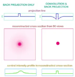
The back-projection from a number of projections reconstructs an image of the atten-uation area. For each projection, the attenatten-uation is homogeneously back-distributed along the projection line, for that, the superposition of the attenuation from different angles causes an evident blur in the reconstruction, as shown in Fig. 1.14(a). Pre-filtering can correct this blur by adding some negative attenuation to eliminate the positive blur in the back-projection process (convolution). In this sense, the filtered back-projection algorithm is derived from the Fourier slice theorem. From the in-verse Fourier transform, the sample function,(x,y)is:

µ(x,y) = Z ∞

−∞

Z ∞

−∞F(u,v)e

i2πwt(ux+vy)

dudv (1.21)

The rectangular coordinate system in the frequency domain, (u,v), can be trans-formed to a polar coordinate system, (w,u), by substituting (u = wcosθ), (v = wsinθ) and differentials by (du dv=wdwdθ). Equation 1.22 can be re-written as:

µ(x,y) = Z 2π

0

Z ∞

0 F

The above integral can be split into two by consideringθ from 0 toπ and fromπ to 2π. By substituting Eqn. 1.6 and using the property of Fourier transformations that [F(w,θ+π) =F(−w,θ)], Eqn. 1.22 can be expressed as:

µ(x,y) = Z π

0

" Z ∞

−∞F

(w,θ)|w|ei2πwtdw #

dθ (1.23)

From Eqn. 1.20, the 2D Fourier transformF(w,θ)can be substituted with the Fourier transform of the projection at angleθ,Sθ(w), as follows:

µ(x,y) = Z π

0

" Z ∞

−∞Sθ(w)|w|e

i2πwt _dw #

dθ (1.24)

The above integral may be expressed in other format, as follows:

µ(x,y) = Z _π

0

Qθ(xcosθ+ysinθ)dθ (1.25)

where

Qθ(t) =

Z ∞

−∞Sθ(w)|w|e

i2πwt _dw

= F−1 (

Sθ(w)|w|

) (1.26)

Equation 1.26 presents a filtering operation. The frequency response of the filter is given by|w|. By substituting Eqn. 1.10 that showsSθ(w)is the 1D Fourier

transfor-mation, Eqn. 1.26 can be re-written as:

Qθ(t) =Pθ(t)h(t) (1.27)

whereh(t) =F{|w|}is the filter function.

Therefore Qθ(t) is called a “filtered-projection". The filtered-projection, Qθ, at

dif-ferent angles, θ, should then be back-projected as in Eqn. 1.25 to form of µ(x,y). In this process, every point (x,y) in the image plane corresponds to a value of t = xcosθ+ysinθ. The filtered-projection, Qθ, contributes its value t to the

re-construction at all of the points (pixels) along a line through the sample µ. This way in the reconstruction process, each filtered-projection,Qθ, is back-projected over

frequencies and increase the high spatial frequencies. The filter, h(t), is depicted in spatial and frequency space in Fig. 1.15. Further information can be found in [Kak and Slaney, 1988; Herman, 1995].

Figure 1.15: Schematic view of the projection filter, h(t), in the spatial domain [Kak and Slaney, 1988].

1.2.7.4 Fan beam

For the parallel projection, the source-detector system linearly scan over a length of projection, at several angle of rotation with a certain interval. This process takes as long as few seconds [Kak and Slaney, 1988]. Using a fan beam radiation, shown in Fig. 1.16, is a much faster solution to generate these line integrals.

1.2.7.5 Cone beam

More recently, high-resolution, inexpensive flat-panel detectors have become avail-able (see section 1.2.4). The configuration of such detectors offers greater dynamic range, however, these detectors require a slightly greater radiation exposure. As shown in imaging geometry of Fig. 1.5, imaging is accomplished by using a rotating sample to which an X-ray source and detector are fixed. A cone-shaped source of radiation can be directed through the sample onto the X-ray detector on the opposite side. During the rotation, multiple sequential planar projection images of the field of view (FOV) are acquired in a complete, or sometimes partial, arc. This proce-dure varies from a traditional CT, which uses a fan-shaped (see section 1.2.7.4) X-ray beam (e.g., in a helical progression [Hu, 1999]) to acquire individual image slices of the FOV and then stacks the slices to obtain a 3D representation. As such in fan beam geometry, each slice requires a separate scan and separate 2D reconstruction, however, the cone beam radiation incorporates the entire FOV and thus only one rotational sequence of the sample is necessary to acquire enough data for image re-construction.

Cone beam CT has been used for medical radiotherapy guidances [Cho et al., 1995] and geological applications [Recur et al., 2014a]. The cone-beam geometry was de-veloped as an alternative to conventional CT using either fan-beam, to provide more rapid acquisition of a data set of the entire FOV and it uses a comparatively less ex-pensive radiation detector. Obvious advantages of such a system, which provides a shorter imaging time, include reduction in distortion in the image due to the sample movements, reduction in deformations, and increased X-ray tube efficiency. How-ever, its main disadvantage, especially with larger FOVs, is a limitation in image quality related to noise and contrast resolution because of the detection of large amounts of scattered radiation.

1

.

3

Conclusion

The applied energy selective techniques, in chapter 3 , 4 and 8 for artefacts correc-tion, and in chapter 5, 6 and 7 for material characterisacorrec-tion, are applied on pro-jection images. These propro-jection images are then reconstructed using the filtered back-projection algorithm described in section 1.2.7. There are techniques that are applied on the reconstructed image, e.g., the material characterisation technique of section 6.3.2, in which case an image reconstruction is required at the very early stage of the image processing.

Energy selective techniques

2

.

1

Introduction

There are two main reasons that motivate undertaking this research on energy se-lective techniques in µCT. Firstly, one of the most important artefacts while working with CT is beam hardening (BH). This artefact is the result of the polychromatic nature of X-rays used in the µCT systems. When an X-ray beam passes through a sample, the lower energy photons are attenuated more readily, as the attenuation coefficient generally decreases with increasing energy. As such, the X-ray beam that passes though the denser part of the sample includes higher mean energy and is less likely to be attenuated, i.e., the beam becomes harder, for that, this effect is called beam hardening artefact. The transmitted intensity recorded on the detectors corre-sponds to the attenuation of a polychromatic radiation (Beer-lamber law in Eqn. 1.3), however standard tomographic reconstruction algorithms assume monochromatic radiation. Since the transmitted intensity data are not linear with the sample thick-ness, the reconstruction produces some visual distortions, such as brighter edges and streaking artefacts. These artefacts make subsequent tomogram segmentation and analysis difficult.

Section 2.2 starts with a demonstration of the physics of the BH artefacts, and con-tinues with an overview of the existing BH correction methods in tomography, with their advantages and disadvantages. I have also chosen several methods and imple-mented them in chapter 3 to assess their accuracy and choose the most appropriate model. Afterwards, using the selected model of chapter 3, a method is presented to compensate the BH for the concentric cylindrical samples in chapter 4.

Section 2.3 begins with a brief review of the material characterisation methods and summarises recent advances in this field. Furthermore, I implemented a pre-reconstruction and a post-reconstruction material characterisation technique inµCT in chapter 6 to compare with the results of my work in chapter 5.

2

.

2

Beam hardening (BH) artefacts and correction techniques

in CT

(a)

(b)

Figure 2.1: Attenuation of a) Silicon and b) Platinum as a function of photon En-ergy (http://physics.nist.gov/PhysRefData/XrayMassCoef/tab4.html). These plots are presented to show that the nonlinear trend of the attenuation coefficients result in the nonlinearity of the beam hardening artefacts (see Eqn. 1.2). Plots of the atten-uation for the energy range of imaging in this thesis, [1, 120] keV, are presented in

When a polychromatic X-ray beam passes through matter, low energy photons are more likely to be attenuated, as the attenuation coefficient generally decreases with increasing energy (see Fig. 2.1). Figure 2.2 shows that as the beam passes through 0.25, 0.5, 1, 2, 4 and 8 mm aluminium filter, the lower energy X-ray is getting attenu-ated more readily, thus, the mean energy of the beam increases gradually, i.e., beam hardening. The rate at which the beam is attenuated decreases at higher energies, so the harder a beam is, the less it is further attenuated. This means that the total attenuation given by the Beer-Lambert law of Eqn. 1.2, i.e., the logarithm of the ratio of the attenuated and incoming X-ray beam (yellow arrows in Fig. 2.2), is not valid for polychromatic X-ray spectra and attenuation estimated in this way is not a linear function of material thickness. This is specified in the beam hardening curves of sec-tion 3.2.2. If this nonlinear effect is not compensated, the reconstructed images will be corrupted by severe edge artefacts and streaks.

Figure 2.2: Effect of beam hardening on reduction of spectra’s photon counts as the beam is passing through the aluminium filters with thickness of 0.25, 0.5, 1, 2, 4, 6 mm shown subsequently in green, blue, red, purple, yellow and black colours. The

spectra is recorded using Amptek CdTe spectrum analyser.

ad-dition, the background attenuation in the convex hull of the sample is overestimated in the reconstructed image. Gompel et al., [Van Gompel et al., 2011] applied an it-erative BH method, explained in section 2.2.3.2, to correct the BH of this image that is shown in Fig. 2.3(iii). Figure 2.3(iv) depicts the line profiles along horizontal line through the reconstructed image of the sample, in which black and grey lines, shown in Fig. 2.3(ii) and (iii), correspond to the beam hardened and corrected reconstruction respectively.

(i) (ii)

(iii) (iv)

Figure 2.3: Illustration of BH effect; (i) a sample made of PMMA and aluminium, (ii) reconstruction including BH artefacts, (iii) BH corrected reconstruction and (iv) a

line through the reconstructions [Van Gompel et al., 2011].

BH artefacts makes the quantitative interpretation of the µCT images and segmen-tation very difficult. This also complicates the calibration and resolution measure-ments. Furthermore, the same materials can result in different intensity-values in projections depending on the surrounding material.

2013; Van de Casteele et al., 2002; Herman, 1979; Krumm et al., 2008; Van Gompel et al., 2011]. This section reviews some of these methods.

There are a number of techniques that can be used to minimise this effect which can be generally categorised as 1) hardware filtration or 2) beam hardening correction software techniques. Typically two types of software BH correction are available: 2a) BH linearisation and 2b) post-reconstruction iterative methods.

2.2.1 Hardware filtering

Hardware filtering is the most common method to narrow the broad spectrum of an X-ray source [Hammersberg and Måns, 1998]. By placing a filter between the source and the sample, the low energy X-rays are attenuated. This helps to achieve a beam with higher mean energy and a narrower energy spectrum. Almost all of the commercial systems use hardware filtering in addition to software beam hardening correction. Fig. 2.4 shows the spectrum of the tungsten source normalised over the area with 0.25 mm Al filtering at 60 keV (blue line) and with 0.25 mm Cu filter at 100 keV (red line). Figure 2.2 shows the variations in spectrum’s photon counts at 100 keV X-ray beam as it passes through the 0.25, 0.5, 1, 2,4 and 8 mm aluminium filters. The figure shows as the spectrum transmitted through the specimen, the ef-fect of SNR varies as well. Without filtering, very soft radiation will not penetrate the specimen and doesn not contribute to the signal information, but it will reduce the dynamic range. The spectrum that passed through 8mm Al filter shows the highest mean energy in the figure.