Abstract: A pump intake system consists of forebay, pumpbay and pipeline arrangements through which water flows in order to meet its demand. Vortices and velocity fluctuations affects the performance of a pump intake system. This paper presents the vortex prediction in a pump sump for varying flow conditions across the pump bay and the bellmouth section, using computational fluid dynamics (CFD) code Flow 3D. Geometry of rectangular type sump was chosen for comparing the physical experimentation with the computational model. The velocity fluctuations, location of vortex formation and its profiles predicted by CFD code was compared with that of the physically observed experiments. The velocity and fluid flow profiles predicted by CFD correlated well with the flow conditions observed during the physical experiments. Further, characteristics of vortex were also studied with respect to the velocity change. Increase in the wobbling phenomenon of the vortex with increase in the flow velocity was also identified with the computational studies. CFD can be used as a tool to study the preliminary design of a hydraulic system for a particular field condition, thus complementing the physical model studies to facilitate the construction of an optimized and effective pump intake system.
Index Terms: bellmouth, pump bay, streamlines, swirl angle, vortices.
I. INTRODUCTION
A pump sump is typically defined as a collecting chamber, through which the fluid flows across its components to supply the requirements. Proper design of the pump sump enables efficient pump performance overcoming irregular flow in the forebay. The intake chamber is often referred to as pump sump. A defective pump sump design may lead to swirls, vortices, velocity fluctuations, bulk circulations and inducestagnant zones during the fluid flow across its components. The formation of vortices and swirls lead to unsteady operation of pumps and causes fall in its efficiency. Swirl formation can cause pre rotation of the flow leading to shock losses at the entry to the impeller. The occurrence of vortices and swirls are generally attributed to improper geometry, uneven velocity distribution and also inadequate depth of submergence.
Revised Manuscript Received on August 5, 2019.
Ajai S., Hydraulic Machinery and Cavitation (HMC) Division, Central Water and Power Research Station, Pune, India.
K. Kumar, Hydraulic Machinery and Cavitation (HMC) Division, Central Water and Power Research Station, Pune, India.
P. M. Abdul Rahiman, Hydraulic Machinery and Cavitation (HMC) Division, Central Water and Power Research Station, Pune, India.
V. S. Sohoni, Department of Civil Engineering, BharatiVidyapeeth Deemed University, College of Engineering, Pune, India.
There are many guidelines for the design of a pump intake, which alone do not always ensure an efficient system. It is appropriate to consider model study since each system is unique to the site and hydraulic conditions. By conducting scaled model studies in the laboratory, the proposed design can be checked and modifications to the intake geometry can be done, depending on the extent of deviations and deterioration in performance. It is general practice, the design of the water intake system or pumping stations is based on the international standards such as American National Standard for Pump Intake Design (1998) as well as the guidelines set by the British Hydromechanics Research Association. These guidelines ensure that the flow across the intake is regulated and also vortices and swirls can be detected and minimized so that unnecessary cavitation, vibrations and undesirable load on the impeller is not produced. However, with the advent of improved technology, it is imperative that the design should be tested for additions and remedial modifications for its performance, according to the specific site conditions.
Various research works carried out for the pump intake studies estimated that 1% of air entrainment can lead to a fall of 10-15 % efficiency in pumps [1]. Air entrainment is the most common effect caused due to the hydraulic disturbances of excessive pre-swirl, vortices that also lead to cavitation, uneven load, noise and vibrations. The most commonly known type is the free surface vortex, which can have varying degrees of intensity– from weak surface vortices to fully developed vortices with a continuous air core that extends from the surface into the pump.
Vortex types usually are identified in the model study by visual observation with the help of dye and artificial debris and identification of coherent dye core to the pump bell or pump suction flange. Vortices are unsteady in strength and intermittent in occurrence. They usually terminate at the suction floor and walls and may be visible only when the dye is injected near the vortex core. The possible existence of sub-surface vortices can be explored by dye injected at all the locations of wall and floor around suction bell where vortices might be formed.
Pre-swirl changes the flow conditions at the pump inlet, which produces changes in the relative impeller speed. Excessive pre-swirl can also result in bearing wear and cavitation across the impeller area. Pre-swirl usually originates from an asymmetric velocity distribution in the approach channel, which evolves into a pre-swirl at the pump inlet. The Hydraulic Institute standards recommend that the swirl angle should not exceed 5°, calculated from the ratio between the tangential velocity and the axial velocity[6].
Roberge (1999) studied
the application of
Vortex Prediction in a Pump Intake System
Using Computational Fluid Dynamics
software FIDAP for predicting the occurrence of vortices in a single pump vertical intake using the Ɛ model and noted prominently the comparison between the results of physical sump model and the CFD simulation [9].
S.G. Joshi and S.N. Shukla (2002) [10] investigated the flow quality entering the pump to get a smooth and swirl free flow over the operating area. J.T Kshirsagar and S. N. Shukla (2008) studied the numerical prediction of air entrainment and submerged vortex with the help of multiphase flow studies, for a single pump rectangular intake model using the
Ɛ turbulence model [7].
Cecilia Lucino and Sergio Lisca y Gonzalo Duró (2010) verified the ability of commercial CFD code, FLOW-3D to predict the formation of vortices in a pump sump and demonstrated that CFD modeling is a useful tool in analysis for pump stations [2].
Tanweer S. Deshmukh and V. K Gahlot (2010) tested the commercially available software of ANSYS CFX and the flow conditions in the pump sump proved to be in good agreement with the experimentally observed flow patterns [12]. S. Pradeep, G. Sayantan, P.G. Prasad and M.S. Mohan Kumar (2012) conducted a detailed numerical simulation of a horizontal pump intake system having multiple pumps using the CFD software code of FLUENT. It included the study of velocity distribution at inlet, swirl angle in the pump suction pipe and streamline patterns in the sump chamber [11]. Kadam Pratap M. and D.S. Chavan (2013) conducted experiments using a single pump intake model under various flow rates to define a set of flow conditions with varying degrees of vortex development. Simulations were done using a commercial CFD software package - ANSYS 13 – FLUENT – V6 for the characterization of flow in the vicinity of the pump intake [8].
Ajai S, Abdul Rahiman PM, Kumar K (2016) verified the effectiveness of computational fluid dynamics FLOW-3D code to simulate and predict the flow conditions in a multi-intake pump sump. The investigation was focused on formation of vortices, swirl flows and mass circulation of the fluid across the pump sump system. The vortex profiles at the pump-bay and near the bellmouth sections were also examined using the computational model of FLOW-3D code [1].
FLOW-3D [5] is general-purpose CFD software. It employs specially developed numerical techniques to solve the equations of motion for fluids to obtain transient, three dimensional solutions to multi-scale, multi-physics flow problems.
The craft of developing these methods is called computational fluid dynamics. A numerical solution of these equations involves approximation of the various terms withalgebraic expressions. The resulting equations are then solved to yield an approximate solution to the original problem. This entire process is known as simulation.
Specifically, CFD is a method of simulating a fluid flow in which standard flow equations such as the Navier-Stokes and continuity equations are discretized and solved for each computational cell. It is important to ensure that the problem being modeled represents the actual physical situation as closely as possible.
FLOW-3D uses the oldest numerical algorithms based on the finite difference and finite volume methods that have been developed for mesh generation.
A proper definition of the boundary conditions at the free surface is important for an accurate capture of the free-surface dynamic. The Volume of Fluid (VOF) method is applied in FLOW-3D for this purpose. It consists of three main components, i.e. the definition of the volume of fluid function, a method to solve the VOF transport equation and setting the boundary conditions at the free surface [5].
II. METHODOLOGY
A simple rectangular type geometry was chosen for the experimental study and the same dimensions were used to prepare the CFD model.
A. Experimental Setup
[image:2.595.306.546.317.417.2]Experimental setup consisted of a tank with three intake pipes, centrifugal pump and control valve to regulate the flow. Fig 1 shows the major components of the experimental setup.
Figure 1 Experimental setup of pump intake
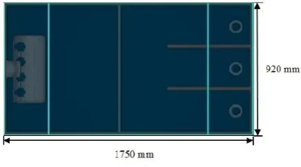
Figure 2 Dimensions of the sump
Dimensions of the sump modeled were 1.75m in length, 0.92m in width and 0.52m in depth. The diameter of the vertical intake pipe was 6 cm and that of the bellmouth entry section was 13 cm. In order to ensure uniform flow across the sump, flow separators and straighteners were provided.
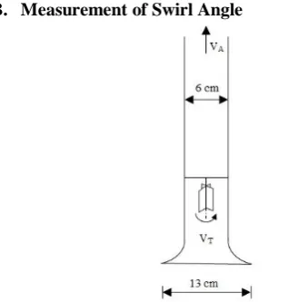
[image:2.595.324.542.459.580.2]B. Measurement of Swirl Angle
Figure 3 Details of the bellmouth and swirl meter
A swirl meter is a device which rotates by virtue of swirl velocities. It was fitted in bellmouth at entrance. Swirl angle is calculated by determining the ratio of tangential velocity to axial velocity.
Axial flow velocity in suction pipe is:
( 1 ) where, Q = Discharge Quantity (m3/s) and
A = Cross Sectional Area (m2)
Tangential Velocity at the tip of the straight blade vortimeter is:
( 2 ) where, = Angular velocity
( 3 ) Where, Swirl Angle in degrees
A simple dye penetration method was used to visualize the vortex structure for flow through the bellmouth section.
C. CFD Model Generation and its Analysis
Geometry is constructed in FLOW-3D by assembling simple solid objects which combine to define the flow domain. The flow geometry is embedded in the computational grid during the pre-processing using a technique called Fractional Area Volume Obstacle Representation (FAVOR). This method computes the open area fractions on the cell faces along with the open volume fraction and reconstructs the geometry based on input parameters.
[image:3.595.324.525.66.204.2]Cubical mesh blocks were generated on the assembled geometry as shown in the fig. 4.
Figure 4 Meshing of the computational model
Pressure inlet and velocity outlet boundary conditions were applied to the inlet and outlet face of the mesh block respectively. The sump was maintained at a constant level of fluid surface level 20 cm for all the simulations and the flow velocity was varied from 0.2 m/s to 2.25 m/s for each of the simulations.
The optimum mesh was chosen as 6 mm, considering the computational time as a major limitation for capturing the expected vortices. The post processing of the result consisted of velocity plots, two- dimensional contours and streamlines of the vortex profiles.
The k-Ɛ turbulence model solver is specified based on the physical nature of the problem; the simulation finish time was specified by assuming the time at which the flow gets completely developed. A steady state was achieved around 50 seconds. All the simulations were made to run till 70 seconds from which the post processing was performed.
The simulations were carried out for similar conditions as that of the physical model.
III. RESULTS AND DISCUSSIONS
Observations were made on the trajectory from the pump bay to the bellmouth sections. Free surface vortices were observed and irregular flow fields at the pump bay observed during the experimental studies were in close approximation with those predicted using CFD.
The dye penetration images captured during the experiments and the streamlines predicted by CFD are shown in fig. 5 and 6.
Figure 5 Surface dimple and vortex observed in the physical model
[image:3.595.322.539.589.809.2]Figure 6 Surface dimple and free surface vortex prediction in the CFD model
The vortex profile initiating from the free surface and then moving through the bellmouth curvature is shown in the fig. 7.
[image:4.595.65.265.51.220.2]The vortex profile with velocity magnitude as iso surface of the submerged vortex and free surface vortex were predicted using CFD.
Figure 7 Vortex profile prediction by CFD
[image:4.595.115.235.316.433.2]The comparisons of swirl angle measured and CFD predicted values are shown in table I and are plotted in the graph below.
Table I Comparison of physical and CFD model results for swirl angle
Simulation Number
Experimental Results
CFD Results
1 4.47 5.34
2 4.83 6.26
3 5.30 7.03
4 8.64 10.67
5 9.55 11.98
6 10.2 14.37
7 12.27 18.68
8 13.28 22.67
9 9.87 14.08
Figure 8 Graph for swirl angles measured in the physical and CFD model
The predicted swirl angle by CFD was higher than that of the measured value by the swirl meter. The presence of the swirl meter or a vortimeter itself dampens the vortices during the process of measurement. The characteristical difference in measuring and predicting the swirl angle through the physical and CFD models was found out to be the major cause for this variation.
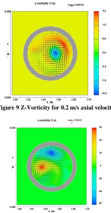
Vorticity for velocities 0.2 m/s, 1.2 m/s and 2.25 m/s are shown through fig. 9-12.
Figure 9 Z-Vorticity for 0.2 m/s axial velocity
Figure 10 Z-Vorticity for 1.2 m/s axial velocity
[image:4.595.335.517.360.707.2] [image:4.595.339.512.365.529.2]Figure 11 Z-Vorticity for 2.25m/s axial velocity
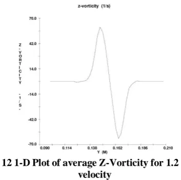
[image:5.595.306.545.49.227.2]Dual vortex with clock wise and anti-clock wise rotation for 1.2 m/s velocity is shown in fig. 12.
Figure 12 1-D Plot of average Z-Vorticity for 1.2 m/s axial velocity
[image:5.595.76.255.50.205.2]Fig. 13 shows the behavior of vortices for the flow varying from 0.2 m/s to 2.25 m/s. The graph was plotted for the diametric points perpendicular to the direction of flow, across the cross sectional area of the pipe.
Figure 13 Z-Vorticity distribution for varying axial velocities
[image:5.595.76.253.254.430.2]The combined graph showing the velocity distribution for various velocity conditions is plotted in fig.14.
Figure 14 Z velocity (w) distribution for varying axial velocities
There is an increasing fluctuation in velocity distribution for each condition with increase in flow.
The range of vorticity fluctuations predicted by CFD and the physically observed conditions are stated in the table II below.
Table II Fluctuating range of Z-Vorticity with respect to axial velocities
Axial Velocity
(m/s)
Reynolds Number
(Re)
Range of Z-Vorticity
(1/s)
Physical Observations
0.2 12000 7 to 8 Minimum to
moderate fluctuations
0.5 30000 20 to 30
0.75 45000 35 to 45
1.20 72000 70 to 95 Adverse
fluctuations
1.75 105000 130 to 190
2.25 135000 200 to 325
Minimal to moderate fluctuations were observed for the flow velocities less than 1 m/s and for the flow velocities higher than 1 m/s highly unsteady and wobbling vortices were identified.
During the physical experiments, it was observed that the vortices had minimum to moderate fluctuations for the flow velocity in the range of 0.2 m/s to 0.75 m/s.
For the higher flow velocities with Reynolds number greater than 100000, the vortex behavior was found to be more fluctuating and adverse wobbling nature was identified. The CFD simulations also predicted the fluctuations and the wobbling nature of the vortex with a close approximation. The flow accelerates through the bellmouth due to its curved shape with reducing cross sectional area and so there is a sudden change in the velocity across the bellmouth. Thus, the fluctuations increase with increase in the fluid velocity as a result of flow turbulence.
The increase in local velocity across the bellmouth section induced low pressure zone, which give rise to flow fluctuations and further the fluctuating vortices.
Diametric points
[image:5.595.62.288.515.692.2]IV. CONCLUSION
During the physical experiments it was found that the condition of the flow approaching the pumpbay and the curved bellmouth plays a major role in the formation of the vortices. The Ɛ turbulence model approximated the flow conditions of the physical model more closely. CFD simulations also demonstrated the capability of this turbulence model in predicting the vortices and velocity fluctuations. The flow conditions such as velocity fluctuations, flow profiles and location of vortices predicted by CFD numerical methods correlates well with the flow conditions observed during the physical experiments. It was also identified that the fluctuating and wobbling behavior of the vortices add complexities in comparing the swirl angle obtained by the physical model and the CFD simulation. The magnitude of the vortices predicted is mostly higher than that of the experimentally measured results which was due to the difference in basic principle of approximation between computational prediction and physical measurement. In addition to free surface vortices the CFD simulated results also predicted the fields of subsurface vortices such as wall and floor vortices. So these features of CFD code can also be used to design well optimized antivortex devices and swirl arresting baffles. Numerical simulations can be performed prior to physical model studies to facilitate construction of an optimized and effective pump intake system, thus saving valuable time and costs.
ACKNOWLEDGMENT
The authors would like to thank Dr. (Mrs.) V. V. Bhosekar, Director, Central Water and Power Research Station (CW&PRS), Pune and Dr. R. G. Patil, Scientist ‘E’, CW&PRS for their constant encouragement and wholehearted support for conducting the above experimentation at Hydraulic Machinery and Cavitation Laboratory.
REFERENCES
1. Ajai S., Abdul Rahiman P M, Kumar K (2016) “CFD nalysis of Multi-Intake Pump Sump System”, Indian Journal of Power and River Valley Development, ISSN: 0019-5537, Issue: September-October. 2. Cecilia Lucino, Sergio Lisca y Gonzalo Duró (2010), “Vortex detection
in pump sumps by means of CFD”, XXIV Latin merican Congress on Hydraulics (IAHR), Punta Del Este, Uruguay.
3. Constantinescu G. S. and Patel V. C. (1998), “Numerical model for simulation of pump-intake flow and vortices.” SCE Journal of Hydraulic Engineering, Vol. 124, No.2, pp 123-124
4. Essam A Khalifa, Mostafa A. Abu-Zeid, S. M. Abdel-Rahman, Sami A. A. El-Shaikh (2014), “Evaluation of the flow characteristics in the intake structure and pump sumps using physical model” , International Journal of Engineering Research and Technology, ISSN 0974-3154 Volume 7, Number 1, pp 79-91.
5. Flow-3D guide, v11.2, Flow Science, Inc., U.S.A.
6. Hydraulic Institute Standards (1998), American national standard for pump intake design, ANSI/HI 9.8., American National Standards Institute, Hydraulic Institute, Washington. DC.
7. J.T Kshirsagar and Shyam N. Shukla (2008), “Numerical prediction of air entrainment in pump intakes”, Proceedings of the twenty fourth International Pump users Symposium.
8. KadamPratap M. and D.S. Chavan (2013), “CFD analysis of flow in pump sump to check suitability for better performance of pump”, International Journal on Mechanical Engineering and Robotics, ISSN (Print): 2321-5747, Volume-1, Issue-2, pp 59-65.
Engineering., Worcester Polytechnic Institute, Worcester, Massachusetts, U.S.A.
10. S.G. Joshi and S.N. Shukla (2002), “Use of CFD for sump flow studies”, National Seminar on ‘Pumps, valves, pipes and accessories’, Mumbai, India.
11. S. Pradeep, G. Sayantan, P.G. Prasad and M.S. Mohan Kumar (2012), “CFD simulation and experimental validation of a horizontal pump intake system”, ISH Journal of Hydraulic Engineering, Vol. 18, No. 3, pp 173-185.
12. anweer S. Deshmukh and V. K Gahlot (2010), “Simulation of flow through a pump sump and its validation”, International Journal of Recent Research and Applied Studies, ISSN 2349-4891, 4 (1), pp 7-17.
AUTHORS PROFILE
Mr. Ajai S. graduated in Mechanical Engineering from Anna University, Chennai and post graduate in Manufacturing Systems and Management from College of Engineering, Guindy. He is with Central Water and Power Research Station, Pune, since 2012. He has experience in calibration of flow meters, testing of control valves and filters. He is actively involved in laboratory testing of submersible pumps, field studies for hydro power plants and CFDstudies of water conductor systems.He has published 4 papers in international journals.
Dr. K. Kumar did his doctorate from National Institute of Technology, Trichirapali (NITT) in 2012; he also holds post graduate degree in Executive MBA from Symbiosis University. He is a Bureau of Energy Efficiency (BEE) certified Energy Auditor and manager, also certified Boiler Operation Engineer (BOE). He is with Central Water and Power Research Station, Pune, since 2006. He has experience in calibration of flow meters, testing of control valves and filters, prototype testing of Hydro turbines. He is actively involved in laboratory testing of pumps as well as field studies for hydro power plants. He has about a dozen technical publications based on varied experience.
Mr. P.M. Abdul Rahiman, graduated in Mechanical Engineering from National Institute of Technology (NIT), Calicut, India in 1987, subsequently obtained M.Tech in Hydro Power from NIT, Bhopal, in 1998. He joined Central Water and Power Research Station, Pune, in 1992 after a brief stint in Fluid Control Research Institute, Palakkad (1987-1992). His field of specialization is prototype and model testing of hydro turbines. He has varied experience in laboratory testing of pumps and flow meters. He has dealt works related to pumping systems; pipeline optimistation and pump intake studies. He has more than 50 papers in various national and international journals and other technical fora during his three decades of professional experience in hydraulics.
Dr. (Mrs.) V. S. Sohoni is a Professor and the Head of Department of Civil Engineering at Bharati Vidyapeeth Deemed University, College of Engineering, Pune. She has a total of 24 publications in various international and national journals and conferences. She is a member of Indian Society for Technical Education and Institution of Engineers (India).She was a shortlisted candidate for ‘Research Internship in Science and Engineering (RISE)’ by Indo-US Science and Technology Forum in 2009. Her areas of interest include Structural Engineering and its applications to Hydraulic Engineering.