Crystallographic Surfaces

(1)

Crystallographic Surfaces

(2)

Dedication

(5)

(6)

Where don’t we find

crystals?

Crystals nets are used extensively in the material sciences as models for highly symmetric atomic structures seen in nature. Such atomic structures were first postulated by scientists studying crystal formations. These formations possessed integer ratios in the angles between their faces and it was from these measure-ments that chemists predicted the symmetries of their atomic structures [6]. In the time since, more sophisticated research methods have been developed for determining these symmetries of crystals, such as x-ray crystallography, giving rise to the field of crystallography. The modern concept for a crystal now refers to material that produces sharp lines in diffraction experiment, which includes a wide class of materials such as salts and metals [6].

There is in particular a strong link between the symmetries of a crystal net and the emergent physical properties of the material [6]. Scientists determine the crystal structure of a material by comparing the result of x-ray diffraction to those expected from different hypothesised structures [6]. For this method to work scientists must have an effective means of enumerating possible crystal structures. There are any number of methods for enumerating crystal structures all of which present their own challenges and rewards [5].

EPINET is one such method developed at the ANU. This process requires the selection of a Triply Periodic Minimal Surfaces sitting in Euclidean 3-space, which acts as a filter over the range of possible crystals [7]. This however leaves an important open question as to how we quantify which crystals are left out by such a filter [6].

Motivated by this problem we here set up the idea of a crystallographic surface as a discrete model for TPMS. We then proceed to set up a theory for the enumeration of crystallographic surfaces modelled closely on T. Sunada’s theory for the enumeration of crystal structures. This framework serves as both a two-dimensional extension of Sunada’s theory as well as a potential framework within which the inverse problem of EPINET can be studied.

(7)

Chapter 1

Motivation

In this chapter we lay out the basic ideas of crystallography, crystal enumer-ation with particular focus on EPINET in order to motivate our algorithm. We give no formal definitions or theorems in this chapter but instead focus on examples; building up the broader intuition that will motivate us through the mathematical work in later chapters.

1.1 The Adventures of Agnes, Barry and Clara,

Episode I

In a far off land...

Barry was feeling very stressed. For reasons best known only to himself and Gauss he had many decades ago set up a farm in the hyperbolic plane. Farming open balls had been all very well at the time but now Barry was starting to get old, and in all this time a whole industry had grown out of his venture. Suddenly there was increasing demand for a whole range of new shapes and hyperbolic farming was starting to outpace Barry’s skill set. It became apparent that he would need to divide his farm up into paddocks to separate the various shapes, but what’s more he’d need a design that could grow with increasing demand. After much thought he decided he would attempt to construct a periodic design, something that could be repeated over and over as the size of the farm needed to increase. Designing this however was no easy task for a two-dimension being like Barry and so he decided to do what all smart people do and ask around for some good ideas.

Barry had a sister, whose name was Agnes for reasons Barry found too horrible to contemplate. She owned a farm in a hyperbolic surface of her own and he appreciated the odd letter they’d often send each other musing the nature of the hyperbolic farming industry. Barry decided in his next letter to write up a description of the problem. A few days later he received a reply and it turned out she was in exactly the same predicament but had been given some rather useful advice by a friend of a friend of hers named Clara. Clara was apparently

(8)

CHAPTER 1. MOTIVATION

an expert at this kind of reasoning and was always willing to offer out advice, so Agnes strongly encouraged Barry to send her a letter.

Barry sent her back a letter thanking her profusely and set to write this Clara a letter. Looking up her details in the directory he discovered something quite astonishing; she lived in a graph! Barry couldn’t possibly imagine how a 1-dimensional creature could possibly solve a two-dimensional problem such as his. But he decided to approach her without prejudice and he wrote the letter. Despite his resolution while writing out the letter he couldn’t help but ask her how she had been able to imagine his sister’s two dimensional problem. He waited for about a good week before he got a reply and what he got was quite astonishing...

To be continued...

1.2 What is a crystal?

To a material scientist a crystal is a three-dimensional arrangement of atoms possessing three independent directions of translational symmetry forming a lattice symmetry group [8]. There are actually any number of ways to imagine a crystal [6]. One such method is using sphere packings [5]. (Picture of sphere packing) Systematic enumeration of crystalline structures has been the focus of a large body of mathematical work and for some time extensive work was done attempting to determine the possible sphere-packings ofR3 [5]. The approach

focused on here uses graphs. (Picture demonstrating this)

In this vein, a crystal is not only a graph, but a graph embedding inE3. The

important features of this embedding are both the positions of the vertices and the isometries of the graph embedding [8]. As stated above crystals are required to have three independent directions of translational symmetry. This symmetry group is referred to as thelattice group [8]. We can from this symmetry group determine the fundamental domain, the smallest section of the graph embed-ding from which the whole embedembed-ding can be reconstructed from the lattice symmetries.

We should stop to take note here that the crystals we are studying are in fact infinite continuations of real world crystal structures. We make this choice in favour of preserving the symmetries of crystals.

Example 1.1. By far the simplest crystal to consider, and one that we will return to frequently, is simple cubic [8]. (Picture of simple cubic.) This can be described as the set of coordinates in R3 with at least two integer coordinates.

It’s lattice group is simplyZ3⊂R3. It’s fundamental domain is simply the unit

cube. When attempting to understand some crystallographic problem it is often helpful to first consider the case of simple cubic in which results can usually be easily visualised.

(9)

crystal having more than one such vertex. In this case a simple example of a crystal with two vertices in its unit cell is diamond. (Picture of diamond) As it’s name suggests diamond is the crystal structure of real world diamonds [8].

1.3 How do we find crystals?

So far the description of crystal we have given is quite simple but surprisingly we can ask some very complicated mathematical questions about them. T. Sunada in his book Topological Crystallography outlines some such problems such as random walks on crystals [8]. One problem of much importance in material science is how to enumerate crystals [5]. Note that this can be broken into two components.

First we have enumerating suitable graphs. These crystal graphs, referred to as topological crystals, are infinite graphs with a symmetry group isomorphic to _Z3 _{identified . Secondly then we have the embedding of this graph. Note} that for some given topological crystal there are an infinite number of ways of embedding this graph as a crystal. In some cases this has physical meaning where we find certain crystallographic compounds with the same topological crystal structure manifest different embeddings depending on the nature of the atoms, or the circumstances of the compounds creation [8].

Example 1.2. A good example of this is diamond. Below we show two embed-dings of the topological crystal diamond. (Pictures)

In other cases however some embeddings are simply physically unrealistic due to features such as closest neighbours that don’t share an edge, or angles between bonds that simply would never occur. This demonstrates the difference between the purely combinatorial or graph properties of crystals and their geometric properties.

T. Sunada in his book Topological Crystallography describes a method of enumerating crystals using the mathematics of covering space theory. This theory covers both aspects of crystal enumeration, the production of topological crystals and the construction of a ‘maximally symmetric’ embedding for this topological crystal. In particular this method is exhaustive over all topological crystals [8]. This maximally symmetric embedding is however limited by the topological symmetries of the topological crystals.

(10)

three-dimensional tilings however has been found to suffer from signifcant com-binatorial explosion as well as redundancies produced by multiple tilings having the same 1-skeleton [3].

EPINET was an algorithm developed at ANU which uses two-dimensional tilings to produce crystals. It was inspired by the fact that crystal nets were known to sit on the p, d, and s surfaces. These surfaces are Triply-Periodic Minimal Surfaces inR3and the EPINET algorithm was developed to enumerate

through all periodic tilings of these surfaces that preserved the three translation symmetries of the surfaces. [7]

(Pictures of these surfaces and the crystals)

By enumerating tilings over these surfaces we can produce any number of crystals. These surfaces are not simply-connected which makes direct enumera-tion using Delaney-Dress symbol theory complicated. Fortunately DDS theory has the added bonus of providing a framework to lift tilings of a surface to a covering space. The problem can be simplified then by making a choice of cov-ering map from the universal cover of these surfaces, the hyperbolic plane. In particular this covering map need to send isometries to isometries so that peri-odic tilings get send to periperi-odic tilings. Then with a choice of map, a subgroup of the hyperbolic isometries are identified with the isometries of the surfaces and enumerating tilings is straightforward from there [7].

1.4 Are all crystals surfaces?

So far however there are gaps in the theoretical foundations of EPINET [6]. The gap we will be focusing on is which class of crystals does EPINET enumerate over. To put it simply we want to understand what crystals fundamentally cannot be produced from a TPMS.

We might wonder why it would be so difficult to prove that no embedding of a crystal on a TPMS exists. For our purposes we will only consider 2-cell embeddings, that is embeddings that can be described by ‘gluing’ faces to the crystal. This problem can then be thought of in two separate components. The first is a purely combinatorial question. If we imagine our crystal as a graph we ask if we can glue faces on a subsection of this graph to form the fundamental domain for a surface stretching over the entire graph.

The second question then is whether the surface formed has an embedding in

E3 that preserves the lattice symmetries of the graph. We could require that

this embedding be an extension of the graph embedding of the crystal. This is, however perhaps a little too strict since such embedding have straight edges which would likely get in the way of producing a minimal surface.

(11)

(12)

(13)

Chapter 2

Sunada’s Method

In this chapter we outline Sunada’s algorithm for enumeratin topological crystals and producing maximally symmetric embeddings. This chapter is based off Sunada’s book topological crystallography [8].

2.1 The Adventures of Agnes, Barry and Clara,

Episode II

In a far off land, Barry receives a letter from Clara, explaining how she sees higher dimensions...

Clara grew up with her mother and siblings in the real line. It had been a straightforward life, Clara had two directions to remember. Things changed quite dramatically when she’d had to move to university. It turned out that university folk were much fancier than the people in her home line and their campus was arranged in something called a graph. It was much in many ways like her home town except for these blasted junction points.

Each junction was connected to six corridors, organised into pairs by three colours. Clara’s navigation skills were at first no match for this strange new structure. She found that everything made perfect sense if she stuck to only red corridors or only blue but once she mixed colours everything got very confusing. Somehow, inexplicably certain sequences of colours would lead her back to where she started, something she spend many nights contemplating at the university pub.

Over time she noticed a pattern; for each of these looping paths she would always travel along an even number of corridors of each colour. This led her to develop a theory. She imagined three different versions of herself, red, blue and green. Each version of her moved along her hometown in between a series of bus stops. They moved independently of one another however only one could move between bus stops at any time. The even pattern now made perfect sense. Each version had to move forwards and backwards the same number of times

(14)

CHAPTER 2. SUNADA’S METHOD

for all three to arrive where they started. Suddenly she found navigating her university was a piece of cake.

It was using this idea, she claimed that she began to understand the real world was three dimensional.

To be continued...

2.2 Combinatorial Graphs

We begin by setting our the basics of combinatorial graph theory as layed out in Sunada’s work. This is perhaps a little basic, but the set up and terminology is useful for understanding Sunada’s algorithm. No proves are reproduced here due to the simplicity of the content.

We begin by defining a graph.

Definition 2.1. Agraph X is a pair (V, E) equipped with three maps,r:E→ E, o:E →V, andt: E→V, such that o◦r=t andr◦r gives the identity map.

Elements of V are referred to asverticesand elements of E aredirected edges.

Undirected edges are equivalence classes of edges under the relation e ∼ r(e). For some edgee∈E, we say thato(e) is theorigin of e,t(e) is theterminus of e, and r(e) is the reflection of e. e is a looped edge if o(e) =t(e). e and e’ are parallel edges if o(e) = o(e’) and t(e) = t(e’).

Definition 2.2. Acombinatorial graphis a graph that has no parallel edges or looped edges.

In particular the reader will note that the topological crystals we will be dealing with will always be combinatorial, however this won’t always be true for the quotient graphs we later introduce.

The following concepts are useful in defining certain topological properties of graphs.

Definition 2.3. Theneighbourhood Nvof a vertex v is the set of alle∈Esuch thato(e) =v.

Definition 2.4. Thedegree of a vertex v, deg v, is equal to|Nv|.

Theorem 2.5. For a graph X = (V,E) the following holds true

X

v∈V

|Nv|=|E| (2.1)

Definition 2.6. Apathin a graph X is a sequence of edges{en}n∈{0,...,N}, such

thato(ei) =t(ei−1) for all 0< i≤N. By abuse of notationo({en}n∈{0,...,N}) =

o(e0) and t({en}{0,...,N}) = t(eN). A path is said to connect its origin and terminus.

(15)

Definition 2.7. Apath-connected graph is a graph such that any two vertices in a graph are connected via a path.

The reader should again note that all crystals considered here are path-connected.

Definition 2.8. Agraph morphismis a map between the vertices of two graphs that also induces a map between the edges of the graph. A graph automorphism is a bijective graph morphism.

Definition 2.9. Anembedding of a graph X inR3 is a mapf :X →R3, such

that everyv∈V is mapped to a pointx∈R3, and everye∈E is mapped to a

path in T from f◦o(e) tof◦t(e).

We now present one definition of a topological crystal we can already under-stand.

Definition 2.10. A topological crystal is an infinite graph X, with a subgroup G(X)∼Z3 of Aut(X) called the lattice group.

This infinite graph is difficult to do calculation on, and so we will introduce the idea of quotient graphs.

Definition 2.11. Aquotient graph X for a topological crystal T is X = T/H, where H is a subgroup of G(X) called the generating subgroup. If H = G(X) then we call X the smallest quotient graph and typically denote it Q.

Example 2.12. We might think back to our example of simple cubic. In this case V =_Z3_{and E =}_V _×_{B, where B is set of standard Euclidean basis vectors} and their negatives. For (v, b) ∈ E we let o((v,b)) = v and t((v,b)) = v + b. Finally r((v,b)) = (v+b,-b), and G(T) is the group of symmetries given by sending v to v + a, and (v,b) to (v+a,b), where a ∈ Z3. Note then any two

vertices are related via a symmetry and so that T/G(T) is then given by V = 0,E = 0×B+, whereB+ is the standard basis for Euclidean space, with o(e) = t(e) = 0 and r(e) = e.

(Picture)

Consider now instead diamond. (Picture of Diamond)

Diamond’s three translational basis vectors are as shown. This results in two vertices in its quotient graph. The quotient graph is shown below.

Sunada’s method enumerates topological crystals using covering space theory so it is now helpful to discuss these concepts using the terminology introduced.

First we build up the concept of a covering graph.

(16)

Thedegree of a covering map is the cardinality of the preimage of any vertex or edge under the covering map, which can be shown to not depend on the choice of vertex or edge.

Definition 2.14. The deck transformation group G( ˜X) of a covering graph is the subgroup of Aut( ˜X) that preserves the covering map. The deck transfor-mation is then a faithful group action over ˜X.

We might notice that we used the same notation for the deck transformation group as the lattice symmetry group. We did this with good reason and now we make clear the relationship between covering graph theory and topological crystals.

Definition 2.15. A covering graph is said to be normal if the orbits under the group action are identical to the fibres under the covering map.

Theorem 2.16. A graph with group action G is a normal covering space over its quotient graph X/G withG(X)= G.

Hence we can now think of a topological crystal as a special kind of covering graph.

Example 2.17. Joel remember here to go through examples for Simple Cubic and Diamond.

We now seek to introduce the Galois Correspondence which is used in Sunada’s method for topological crystal enumeration. We will first set this up using the fundamental group, and then using graph homology which is used more in prac-tice.

We start then by building up the fundamental group.

Definition 2.18. A geodesic is a path that does not backtrack over itself.

Definition 2.19. A deformation retraction over paths is an equivalence relation whereAer(e)B ∼ABUnder this relation all paths are equivalent to a geodesic.

Definition 2.20. The fundamental group with base pointx0,π1(X, x0) is the group of deformation retraction classes of loops under concatenation, with the empty path as the identity.

Note that for any x0, y0 ∈ X, there is an isomorphism between π1(X, x0) produced simply by conjugating by a path between the two points so when working from a purely algebraic standpoint we may refer to the fundamental group of a graph.

We now build up the Galois correspondence.

Theorem 2.21. A path starting at x in X can be lifted up uniquely to a path inX˜ provided a starting pointx0∈X˜ is chosen.

Theorem 2.22. The covering map induces an injective group homomorphism between the fundamental groups. This also tells us thatπ1( ˜X, x0)is isomorphic

(17)

Definition 2.23. For a graph X a universal cover of X is the covering graph corresponding to the trivial subgroup. It follows then that this covering graph is simply connected.

Theorem 2.24. Any two universal covers of X are isomorphic as graphs.

We may now state the Galois correspondence.

Theorem 2.25. There is a bijective correspondence between subgroups ofπ1(X, x)

and covering spaces of X up to graph isomorphism. Furthermore given a normal covering spacep: ˜X →X the following equation holds true

G( ˜X)∼= π1(X) p∗(π1( ˜X))

. (2.2)

This theorem can be used to enumerate through all possible covering spaces over a finite graph. This is achieved by first computing the universal cover which is in practice quite easy to do. We can then quotient this universal by the subgroup of the deck transformation group corresponding to the generating subgroup of any covering graph to produce this covering graph.

Example 2.26. Joel remember to include examples here for simple cubic and diamond.

In particular this leads us to a new defintion of a topological crystal.

Definition 2.27. A topological crystal is an infinite-fold covering space of a graph such that the deck transformation group is a free abelian group of rank 3.

Note that since our covering spaces always have abelian deck transformations it is actually often more useful to use graph homology. In particular homology calculations are generally easier than calculations involving the fundamental group.

We begin by setting up the basics of graph homology.

Definition 2.28. The zeroth-order chain groupC0(X) is the free abelian group of vertices. The first-order chain group C1(X) is the free abelian group of directed edges with r(e)∼e−1_.

Definition 2.29. The boundary map of a graph is a homomorphismC1(X)→ C0(X) that sends e tot(e)−o(e).

Definition 2.30. The homology group of a graph is the kernel of the first-order boundary map.

We then note the following useful fact.

(18)

Furthermore the first-order homology group is a free abelian group and hence we can define the betti number of a graph.

Definition 2.32. The betti number of a graph, b1(X), is the rank of its ho-mology group.

Theorem 2.33. For a graph X = (V,E) the following relationship holds true,

|V| −|E|

2 = 1−b1(X) (2.3)

Definition 2.34. An abelian covering graph is a covering graph whose deck transformation group is abelian.

Considering then the Galois correspondence for the fundamental group we find the following definition useful.

Definition 2.35. For a graph X the universal abelian cover of X up to graph isomorphism is the covering graph corresponding to the commutator subgroup ofπ1(X, x0).

Furthermore we note that if ˜X is the universal abelian cover thenG( ˜X)∼= H1(X).

We now wish to state the Galois correspondence for homology but first we will require the following two lemmas.

Theorem 2.36. The covering mapp: ˜X →X induces a homomorphism p∗: H1( ˜X)→H1(X).

Theorem 2.37. Letp: ˜X→X be an abelian covering graph, andν :π0(X, x0)→ G(X)be the homomorphism with kernelp∗π0( ˜X,x˜0)from the Galois

correspon-dence. If c is a closed path in X, and˜cis a lift over c toX˜, thent(˜c) =µ(c)o(˜c), whereµ is the homomorphismH1(X)→G( ˜X)induced byν.

From these the following follows.

Theorem 2.38. Letp: ˜X→X be an abelian covering graph, andν :π0(X, x0)→ G(X)be the homomorphism with kernel p∗π0( ˜X,x˜0). Thenkerµ=p∗H1( ˜X),

whereµ is the homomorphism induced byν.

We then refer to the image of this homomorphism as the vanishing subgroup, H. Finally we obtain the Galois correspondence for abelian covering graphs.

Theorem 2.39. There exists a bijective correspondence between subgroups of

H1(X) and abelian covering spaces of X given by the generating subgroup. In

particular

G( ˜X)∼= H1(X) p∗(H1( ˜X))

. (2.4)

(19)

2.3 Enumerating Crystals with Covering Space

Theory

We break the process of enumerating crystals into two distinct components. First the enumeration of topological crystals and the construction of a graph embedding. We first begin by enumerating possible starting quotient graphs, X = (V,E). We only consider finite connected graphs due to physical relevance. We start by fixing the betti number, b1(X). Note that to get a topological crystal we will need to haveb1(X)≥3.

We claim that we need only enumerate graphs where every vertex is at least degree 3. To justify this we note that we can delete a vertex of degree one without changing the betti number. Additionally since b1(X) ≥ 3 and our graph is path-connected we can delete a vertex of degree 2 and replace the two adjoined edges with a single connecting edge without changing the betti number. Hence any graph can be reduced to a graph with minimal degree 3.

Since P

v∈V |Nv| = |E|, we can deduce 3|V| ≤ |E|. Combining this with |V| − |E₂| = 1−b1(X) we obtain |V| ≤2b1(X)−2, and |E| ≤3b1(X)−3. So given a fixed choice ofb1(X) we have a finite number of possible vertices with degree at least 3 we can enumerate through all possible graphs that satisfy the above conditions.

The next step is once we have chosen a quotient graph we compute its first-order homology group. A simple way to do this is to construct an adjacency matrix. This is obtained by assigning each column in a matrix to a vertex and every row an edge. For each edge e a 1 is placed in the column corresponding to t(e) and -1 for o(e). This matrix represents the boundary mapC1(X)→C0(X). We can then calculate the kernel for this boundary map using linear algebra techniques.

Example 2.40. Given the following graph X we can compute the adjacency matrix.

∂1=

1 1 1 1

−1 −1 −1 −1

Now we need only compute the kernel.

N ul(∂1) =b

    −1 1 0 0     +c     −1 0 1 0     +d     −1 0 0 1    

From this we deduce thatH1(X) is generated by the pathsa−1b,a−1c and a−1d.

Now that we haveH1(X) we need to look for possible generating subgroups. That is we want any subgroup H ⊂H1(X) such that

H1(X) H ∼=Z

3_{. There will}

in general be infinitely many such groups but we can introduce a constrait to enumerate over. If x=P

e∈Eaee is an element of the first-order chain group then let |x| = P

(20)

h(H) =minS generates Hh(S). We note that if we fix h, then there are finitely mainly S such that h(S)≤h. Since H is determined by a choice of S it then follows that there are finitely many H such thath(H)≤h. We can then use h as a constraint to enumerate over.

Example 2.41. In the case from above we observe thatH1(X)∼= Z3 so the

only option for H is the trivial subgroup. We then have that the only crystal we can choose is the maximal abelian cover which is in fact diamond.

We could at this point attempt to construct an explicit representation for the topological crystal corresponding to H. In fact we will show that Sunada’s method enables us to skip this step.

We have now a method for enumerating topological crystals and so the final step necessary is to construct an embedding. Before we defined an embedding for a graph, but for a topological crystal we also want to require the embedding to realise all lattice symmetries as isometries.

Definition 2.42. An embedding for a topological crystal T = (V,E) is a graph embeddingφ that sends all edges to straight line segments and which induces a homomorphism ρ:G(X)→R3, such that if v∈V,σ∈G(X) thenφ(σv) =

φ(v) +ρ(σ).

In the case of Sunada’s embedding we seek to construct an embedding that is ‘maximally symmetric’. To make sense of this definition we first define the symmetry group of a topological crystal.

Definition 2.43. The symmetry group of a topological crystal is given by Aut( ˜X/Q) ={f ∈Aut( ˜X|f ◦p=p◦f0,for somef0 ∈Aut(Q)}.

Intuitively we can think of this as the set of graph symmetries that perserves the quotient graph. The definition of a maximally symmetrical embedding then follows thusly.

Definition 2.44. A maximally symmetric embedding of a topological crystal is an embedding, φwhich induces a homomorphism ρ: Aut(T /Q)→ R3 such

that ifv∈V,σ∈Aut(T /Q) thenφ(σv) =φ(v) +ρ(σ).

Sunada’s method allows us to construct a maximally symmetric embed-ding, with a few pathological cases where the method fails. Before introducing Sunada’s method we first wish to show that if we want to prove that an embed-ding is maximally symmetric, it is sufficient to prove the following conditions.

X

e∈Nv

φ(e) = 0, for every x∈V (2.5)

X

e∈E0

hx, v0(e)iv0(e) =cx, (2.6)

(21)

If an embedding satisfies the first condition we call it aharmonic realisation. If an embedding satisfies both conditions we call it a standard realisation. We will first begin by proving that two harmonic embeddings are related via an affine transformation. We will then use this to prove that two standard realisations are related via a similitude. Finally we will show that if v∈V,σ∈Aut(T /Q), and phi at standard realisation, thenφ(σT) is also standard realisation which proves thatφis a maximally symmetric.

First we prove that harmonic realisations are unique up to affine transfor-mation. For this we use the following Lemma.

Theorem 2.45. Two harmonic realisations that share the shame induced ho-momorphism φ:G(X)→R3 are related via a translation.

Proof To prove this we begin by showing that a harmonic realisation min-imises the expression

X

e∈E0

||φ(e)||2. (2.7)

Letφbe a harmonic realisation andφ’ another embedding of the same topolog-ical crystal sharing the same induced homomorphism and letf =φ0−φ.

X

e∈E0

0

||φ00(e)||=

X

e∈E0

(||φ0(e)||2+ 2hφ(e), f(t(e))−f(o(e))i+||f(t(e))−f(o(e))||2)

= X

e∈E0

(||φ(e)||2+ 2hφ(e), f(t(e))i −2hφ(e), f(o(e))i+||f(t(e))−f(o(e))||2)

= X

e∈E0

(||φ(e)||2_{+ 2}_h_φ(₋_{e), f}_(t(₋_e))_{i −}₂_h_{φ(e), f}_(o(e))_i₊_||_f_(t(e))₋_f_(o(e))_||2₎

= X

e∈E0

(||φ(e)||2−4hφ(e), f(o(e))i+||f(t(e))−f(o(e))||2)

= X

e∈E0

||φ(e)||2₊ X

v∈V0

X

e∈Nv

hφ(e), f(v)i+ X e∈E0

||f(t(e))−f(o(e))||2

= X

e∈E0

||φ(e)||2₊ X

e∈E0

||f(t(e))−f(o(e))||2

≥ X

e∈E0

||φ(e)||2

(2.8)

Hence we have that a harmonic realisation minimises the above expression. Consider that if the other embedding is also a harmonic realisation then we must require

X

e∈E0

||f(t(e))−f(o(e))||2_{= 0}

f(t(e)) =f(o(e))

(2.9)

(22)

Theorem 2.46. The harmonic realisations are unique up to affine transforma-tions.

Consider two harmonic realisations φand φ0 with induced homomorphisms, ρ and ρ0. We can find a matrix A such that Aρ = ρ0. Consider then the embedding Aφ. Note that P

e∈NvAφ(e) = A

P

e∈Nvφ(e) = 0. Aφ is then a

harmonic realisation with the induced homomorphism ρ0. Using the previous result then we have thatφ0 =Aφ+b.

We now prove that two standard realisations are related by a similitude.

Theorem 2.47. The standard realisations of a topological crystal are unique up to similar transformations.

Proof We will prove this by first showing that a standard realisation minimises the term vol(D)−2

3P

e∈E0||v0(e)||

2_{, where D is the parallelopiped formed by}

the generating set of ρ(G( ˜X). Supposeφ is a standard realisation and φ0 is a harmonic realisation of the same topological crystal. Since both are harmonic realisations we know that φ0 = Aφ+b. We make a choice of coordinates to obtainφ= (φ1, φ2, φ3),

X

e∈E0

0

||φ0(e)||2₌ X

e∈E0

||Aφ(e)||2

= X

e∈E0 3 X i=1 3 X j=1 Aijφj

3

X

k=1 Aikφk

= 3 X i=1 3 X j=1 3 X k=1

cAijAikδjk

=ctrace(ATA)

(2.10)

We then consider the following inequality, the proof of which is given in Sunada’s book,

tr(ATA)≤d(det(ATA)) (2.11)

And in particular the equality is realised if and only ifA=λI. Applying this we obtain

X

e∈E0

0

||φ0(e)||2_≥_cddet(AT_A)1 3

=cddet(A)23

(2.12)

We now consider the second requirement forφbeing a standard realisation can be written as

X

e∈E0

(23)

This then gives us

X

e∈E0

φi(e)2= 3c

X

e∈E0

0

||φ0(e)||2_≥ X

e∈E0

(||φ(e)||2₎vol(D0) 2 3

vol(D)23

vol(D0)−23 X e∈E0

0

||φ0(e)||2_≥_vol(D)−2

3 X

e∈E0

||φ(e)||2

(2.14)

Hence we have that a standard realisation minimises this value. Suppose both embeddings are standard realisations. Thus we require that AT_A₌_λI _which gives us that A must be a scalar times an orthogonal matrix. Finally this tells us thatφ0 andφare related via a similitude.

And now the final step is to prove that a standard realisation is indeed maximally symmetric.

Theorem 2.48. A standard realisation is maximally symmetric.

Proof Suppose that φis a standard realisation of a topological crystal with covering map p:T →Q, with induced homomorphism ρ. Letg ∈Aut(T /Q). We want to showg◦φis a standard realisation of the same topological crystal. The first step is to prove that it is an embedding of the same topological crystal. Letσ∈G(T). First we consider that

(g◦φ)(σv) =φ(gσg−1gv) =φ(gv) +ρ(gσg−1) = (g◦φ)(v) +ρ(gσg−1)

(2.15)

We now wish to show thatgG(T)g−1₌_G(T_{). Suppose}_σ_∈_G(T_).

(gσg−1)◦p=g−1◦σ◦g◦p =g−1◦σ◦p◦g0 =g−1◦p◦g0 =g−1◦g◦p =p

(2.16)

Hence gσg−1_∈_{G(T) and} _gG(T_)g−1₌_G(T_{) as required. This finally gives us} thatg◦φis an embedding of the same topological crystal. Lastly we need only show that g◦φis a standard realisation. First we observe

X

e∈Nv

φ(g(e)) = X e∈N_g−_{1 (}_v₎

φ(e)

= 0

(24)

and then we observe

X

e∈E0

hx, φ(g(e))i= X e∈g−1_(E)

hx, φ(g(e))i

=cx

(2.18)

And so we see here thatg◦φis a standard realisation of the same topological crystal asφ and henceg◦φmust be equal φcomposed with a similitude. By sending g to this similitude we obtain our induced homomorphism and henceφ is maximally symmetric.

2.4 Sunada’s Algorithm

We will now describe Sunada’s algorithm for constructing standard realisations of topological crystals. Given a topological crystal T with quotient graph X we can constructC1(X,R). This is a vector space and we define on it the following

inner product.

he, e0i=

    

1, ife=e0 −1, ife=r(e0) 0, otherwise

(2.19)

In describing this algorithm we will abuse notation and image paths as directly sitting in C1(X) which we in turn imagine sitting in C1(X,R). Using this

inner product we now let p0 be the orthogonal projection onto the subspace perpendicular to the subspace generated by H, inH1(X,R).

We now make a choice of vertex, v in the topological crystal and letφ(v) = 0. We now choose a pathx0_v originating at v for each vertex v’. We then assign φ(v0) =p0(p∗(x0v)). We then letφ(e) be sent to the straight line segment joining o(e) and t(e).

Theorem 2.49. Sunada’s method does not depend on the choice of pathx0

v.

Proof Let x and y both originate at v and terminate at v’. We then consider the loopxy−1_{. Note that since this is a loop it is contained in}_H

1(T). We then have thatp∗(xy−1₎_∈_H _{which tells us that}_xy−1_{is perpendicular to the image} of the orthogonal projection and hence sent to 0.

p0(xy−1) = 0 p0(x)−p0(y) = 0

p0(x) =p0(y)

(2.20)

Hence we have proven that Sunada’s method does not depend on the choice of path.

(25)

Proof First we show that Sunada’s method produces an embedding of the topological crystal. Supposeσ∈G(T). Let y be a path betweensigmavand v.

φ(σv0) =p0p∗(xσv0)

=p0p∗(y+xv0)

=p0(p∗y) +p0(p∗xv0)

(2.21)

Note that p∗(y) is a loop based at p(v). Hence eitherp0p∗(x0v) = 0 orp∗(x0v) is in the image of the orthogonal projection in which case since it gets send to a the image ofφthe induced homomorphism. Hence

φ(σv0) =φ(v0) +b (2.22)

where b is in the image ofφ. Now we show that Sunada’s method is harmonic. Let c ∈ H1(X,Z). First consider the case that c does not pass through the

vertex. Then

he, ci= 0,for alle∈E0

hX e∈E0

e, ci= 0 (2.23)

Now consider the case that c does pass through the vertex. Then it for every edge component that terminates on the vertex we must have one that originates on the vertex. Hence

hX e∈E0

e, ci= 0 (2.24)

Hence we have that

hX e∈E0

e, ci= 0,for allc∈H1(X,Z). (2.25)

Since H1(X,Z) spans H1(X,R) we then have that Pe∈E0e is orthogonal to

H1(X,R) finally giving us that

p0(

X

e∈E0

e) = 0 (2.26)

Finally we show that Sunada’s method is standard.

Example 2.51. Consider the nice example of diamond. The quotient graph is shown below.

We can choose a basis for C1(X,R), {a, b, c, d}. We now wish to choose

a basis for H1(X,R) given by {a√−b

2, b_√−c

2,

a+b−c−d

2 }. Note that this is an or-thonormal basis. We then set atom 1 to the origin. We can then express every other atom via a word in {a, b, c, d}. We then need simply to project each

ele-ment in{a, b, c, d} into H1(X,R). We then get the followinga→

_√1 2 0 1 2

, b→

−_√1 2 0 1 2

, c→

0 1 √ 2 −1 2

(26)

So now we have that all atoms in diamond are realised as integer combina-tions of these vectors. This is a particularly nice example as diamond in fact does exhibit this maximally symmetric embedding in nature.

Note that Sunada’s method is harmonic and hence minimises the term

P

e∈E0|φ(e)|

2_{, which essentially minimises the lengths of edges given a fixed}

(27)

Chapter 3

Crystallographic Surfaces

In this chapter we set up the theory of Crystallographic Surfaces closely following Sunada’s theory of Topological Crystals. This serves as both a two-dimensional extension of Sunada’s theory as well as a model for computing Triply-Periodic Minimal Surfaces for our inverse EPINET algorithm. The algorithmic approach and layout is based off Sunada’s book Topological Crystallography [8]. Some of the theorems and defintions are based off B. Mohar and C. Thomassen’s book Graphs on Surfaces [2]. Further definitions are based off A. W. M. Dress’s paper [1] and O. D. Friedrichs paper [4].

3.1 The Adventures of Agatha, Barry and Clara,

Episode III

Barry was quite struck by Clara’s story and he wrote a letter explaining back to her his paddock as a graph that sat inside a pairs of numbers which he understood to be a coordinate system. He didn’t really feel that a coordinate system was very useful however in designing a paddock structure in the first place and he stressed this in his letter.

It was many days and nights before she replied but finally she did and the answer to his problem was pleasantly simple. It said to imagine himself at the centre of each paddock performing a Barry-centric subdivision. This would break each paddock up into triangles, but as the letter pointed out each triangle could be assigned an edge of exactly one of three colours based on a simple rule. This in terms allowed Barry to simplify his picture so that each triangle was the vertex of a graph which had three edges each one a different colour leading to each of its three neighbours. It turned out that Barry could rotate around either a corner in the fence, a length of fence or a paddock simply by choosing two colours and alternating them repeatedly. If Barry could imagine a graph that satisfied these simply conditions then it could be built up into a paddock structure. Hence he now had a simple method of creating his paddock structure. It turned out his sister had been given the same advice and sent him back

(28)

CHAPTER 3. CRYSTALLOGRAPHIC SURFACES

some plans she had been drawing up for herself. Her plans were confusing to Barry however, it seemed that certain loops in her graph didn’t correspond to the alternating colour paths...

3.2 Crystallographic Surfaces

We start by defining the notion of a 2-cell complex as a purely combinatorial object that we will use as the basis for our conception of a surface.

Definition 3.1. A 2-cell complex is a triplet (V, E, F) such that (V, E) is a graph along with functions∂f :Z/nfZ→E, andρ:F →F such that

∂f(i+ 1)⊂N(t(∂f(i)))

Im(∂f) =Im(∂ρf)

If∂f(i) =∂ρf(j) then∂f(i+ 1) =∂ρf(j−1)

(3.1)

We refer toS1= (V, E) as the graph of the 2-cell complex. Elements of F are called orientated faces. Imδfis referred to as the boundary of the orientated face f. A non-orientated face is an equivalence class under the equivalence relation f ∼ρf.

Example 3.2. As a simple example consider the 2-boquet graph with two faces with boundaries a and b.

Definition 3.3. The neighbourhood of an orientated edge Ne is the set of orientated faces f such thate∈Imδf.

We now introduce an analogous concept to covering graph theory for 2-cell complexes.

Definition 3.4. A 2-cell complex is a mapp: ˜S→S which is a covering graph when restricted to the graphs ˜S1 _and_S1_and

ρp(f) =p(ρf)

Imδp(f)=p(Imδf)

(3.2)

p is a bijection onNe.

The deck transformation groupG( ˜S) is the same asG( ˜S1) for the covering graph.

Definition 3.5. The fundamental group with basepoint v0 ∈ V for a 2-cell complex (V, E, F) is given by

π1(S, x0) =

π1(S1, v0)

H , (3.3)

(29)

Theorem 3.6. For a 2-cell complex S = (V,E,F) and basepoint v0∈V, there

is a bijective correspondence between subgroups of π1(S, v0)and covering 2-cell

complexes of S. Furthermore for each covering 2-cell complex p: ˜S →S, with basepoint ˜v0∈p−1(v0), we have

G(X)∼= π1(S, v0) p∗(π1( ˜S,˜v0))

(3.4)

Proof We already have the Galois correspondence for the covering graph p : ˜S1 _→ _S1_{. Noting that by definition} _{G( ˜}_{S) =} _{G( ˜}_S1_{). Hence letting H be} the normal subgroup generated by boundary cycles conjugated by appropriate paths, and similarly for ˜H we obtain

G(X)∼= π(S 1_{, v}

0)

p∗_{π( ˜}_S1_,_˜_v 0)

∼ = π(S

1_{, v} 0)/H

p∗_{π( ˜}_S1_,_˜_v 0)/H

∼

= π(S

1_{, v} 0)/H

p∗_{(π( ˜}_S1_,_v_˜ 0)/H)˜

∼

= π(S, v0) p∗_{π( ˜}_S,_˜_v

0)

(3.5)

We now set up homology for 2-cell complexes.

The zeroth- and first-order chain groups of a 2-cell complex are simply be the zeroth- and first-order chain groups of its graph. Similarly the first-order boundary map of a 2-cell complex is the first-order boundary map of its graph.

Definition 3.7. The second-order chain group of a 2-cell complex, C2(X) is the free abelian group over orientated faces with the identificationρf =−f.

Definition 3.8. The second-order boundary map of a 2-cell complex is given by

∂2=Pe∈Im(∂f)e.

Definition 3.9. The first-order homology group of a 2-cell complex S is given by

H1(S) =ker∂1/Im∂2. (3.6)

We then still obtain the Galois correspondence for abelian covering 2-cell complexes.

Theorem 3.10. There exists a bijective correspondence between subgroups of

H1(S) and abelian covering 2-cell complexes of S, furthermore for an abelian

covering 2-cell complex p: ˜S→S we have the following

G( ˜S)∼= H1(S) p∗_H

1( ˜S)

(30)

Proof This proof follows from the case for graphs analogous to the case for the fundamental group.

We now introduce a helpful concept called the characteristic.

Definition 3.11. For a finite 2-cell complex the characteristic χ is given by χ=rankC0−rankC1+rankC2.

We now introduce our equivalent of a crystal for 2-cell complexes.

Definition 3.12. A crystallographic 2-cell complex is an abelian covering 2-cell complex over a finite surfacep: ˜S →S such thatG( ˜S) is a free abelian group of rank 3.

We now note that for our purposes we want to focus on triply-periodic surfaces and so we now define an orientable surface as a special kind of 2-cell complex.

Definition 3.13. A 2-cell complex is an orientable surface when |Ne|= 2, for all edges e.

For every vertex v, there exists a permutationσvonNvsuch for eache∈Nv, there is a face neighbouring both e and r(σve). Furthermore an orientated surface is non-regular if there exists an edge e and an orientated face f such that Ne={f, ρf}.

Example 3.14. Consider again the 2-boquet graph with three faces with bound-aries a, b and ab.

For a non-regular example consider the below graph with three faces attached to a, c and abc.

Note that since an edge has exactly two neighbouring orientated faces it follows that both faces can be recovered from the rotation scheme. We can use this to produce a method of enumerating orientated surfaces over a finite graph.

Definition 3.15. A rotation scheme on a finite graph is a collection of permu-tationsσv on eachNv.

Theorem 3.16. A rotation scheme induces an orientated surface on a graph.

Proof Select a vertex v, and then select an orientated edge e in its neighbour-hood. Let this be the first edge in our path. We can then select the vertex t(e) and then the orientated edgeσt(e)r(e). We then add this new edge to our path and keep going. This is a finite graph so we must eventually reach our original edge. At this point we have a cycle which we identify as the boundary of a new face f. We can then repeat this procedure starting from a different vertex, edge pair, remembering not to repeat the same cycle twice until we have all faces.

Definition 3.17. For a finite orientable surface the genus is given byg= 1−χ₂

(31)

Proof

rankH1(S) =rankkerδ1−rankImδ2

=rankC1(S)−Imδ1−rankC2(S) + 1

=rankC1(S)−rankC0−rankC2(S) + 2

= 2−χ

= 2g

(3.8)

Here will denote a finite surface of genus g byMg.

3.3 Enumerating Crystallographic Surfaces

We now wish to construct a theory for enumerating crystallographic surfaces analogous to Sunada’s method.

The first step is to enumerate over finite graphs X. For each graph X we enumerate through all choices of rotation schemes to produce a finite surface Mg.

Once we have a choice of surfaceMg we can enumerate through all crystal-lographic surfaces over this surface by calculating the homology groupH1(Mg) and enumerating through all subgroups to produce a covering surface.

This provides a complete process for enumerating crystallographic surfaces. It now remains to develop a theory for embedding these surfaces.

Definition 3.19. An embedding of a crystallographic surface inR3is a

collec-tion of injective funccollec-tionsfV :V →R3,fE→P(R3) andfF :F →P(R3) such

that, fe(e) is a line segment joining fv(o(e)) and fv(t(e)), andff(f) is a disc bounded byfe(δ(f)).

Note that this definition has a lot of degrees of freedom associated with how we embed the vertices, edges and faces. We wish to have a more combinatorial process and so we introduce the concept of flags.

Definition 3.20. A flag on a CW-complex is a triplet (v, e, f) such that

eitherv=o(e) orv=t(e)

e∈Imδf

(3.9)

We now introduce a more combinatorial notion of an embedding.

Definition 3.21. An barycentric embedding of a crystallographic surface is collection of injective functions,f_V0 :V →R3, fE0 :E →R

3 _f0

f :F →R 3 _such

that for any two flags c and c’, the triangles formed by f’(c) and f’(c’) only intersect on at most a shared boundary edge.

We will now show that this concept indeed deserves the term embedding.

(32)

Proof The induced functionfV is simplyfV0 . fE maps e to the union of the straight line segment joiningf_V0 (o(e)) andf_E0 (e) with the straight line segment joining f_E0(e) and f_V0(t(e)). fF maps f to the union of the triangles formed by f(c), where c is a flag.

Since this embedding is described in terms of ’flags’ we wish to derive a combinatorial structure over these flags to make this process more combinatorial. Our first step is to define what we will refer to as reflection.

Theorem 3.23. If we fix the edge of a flag and either the vertex or face, then there is only one choice for the remaining element.

Proof We will consider both possible cases. First consider the case that the vertex and edge are fixed. We then have two choices for the face from the neighbourhood of the edge. Suppose instead we fix the edge and face. We then have two choices for the vertex as either the origin or terminus of the edge.

We will now define reflections on our flags in terms of an action of the free Coexter group with three generators.

Definition 3.24. The reflection group action on a surface is the action ofhσii on the set of flags on a surface where

σ0cswitches the vertex,

σ1cswitches to the adjacent edge with the same face in the rotation scheme of the vertex.

σ2cswitches the face.

We now show that these actions deserve the term reflection.

Theorem 3.25. For all i, σ2 i = 1.

Proof We claim that the case follows from the previous theorem forσ0andσ2. Forσ1we consider that this action switches to the adjacent edge with the same face in the rotation scheme of the vertex. Note that there is a unique choice of such edge since by the definition of a surface each oriented edge belongs to two oriented faces, one shared withr(σe) and one shared withσ−1_r(e).

Definition 3.26. For the set of flags on a surface the functionmij : C→ N,

i, j∈ {0,1,2} is given by

mij(C) =min{m|(σiσj)mc=c}

Theorem 3.27. mij(C) = 2 when|i−j|>1.

This object can now be used for

(33)

Note that there is a representation of this embedding using the Delaney-Dress symbol.

Note however that a non-regular surface does not have a barycentric embed-ding.

Example 3.29.

Note that we can form a representation ofC1(X0,R) usingC×σ. However

there is no convenient way of determining H1(X,R).

Definition 3.30. For a surface, the Delaney-Dress graph, XD is formed by assigning a vertex to each flag and an edge to each reflection between flags. We note that the each edge has a number {0,1,2} which we refer to as the colour of the edge.

Theorem 3.31. Ifp: ˜S→Sis a covering surface, then there is a corresponding covering graph p: ˜XD_→_XD_.

Proof This follows from the observation that a flag is a ordered triplet of vertex, edge and face all of which are sent via covering map.

Definition 3.32. An orbit is a simple loop through the Delaney-Dress graph made up of an alternating pair of colours.

Theorem 3.33. There is a one-to-one correspondence between orbits and the elements of a surface.

Proof Note that a pair of colours corresponds to switching between a pair of elements for a flag. The remaining element therefore is preserved. This defines the forward correspondence. Work out details later.

Definition 3.34. The lattice group of the Delaney-Dress graph of a covering surface is the deck transformation group of the induced covering graph.

Definition 3.35. A Delaney-Dress embedding is a function f :C →_R3 _such that the lattice group is send to a group of lattice isometries.

Theorem 3.36. An embedding of a Delaney-Dress graph induces a barycentric embedding on a crystallographic surface.

Proof First we consider a regular surface. In this case we simply embed each surface element at the centre of its orbit.

Definition 3.37. The standard Delaney-Dress embedding of a regular crystal-lographic surface is the embedding induced by the standard realisation of it’s Delaney-Dress symbol.

(34)

(35)

Chapter 4

Inverting EPINET

In this chapter we seek to apply the theory of crystallographic surfaces to the inverse problem for EPINET.

4.1 The Adventures of Agatha, Barry and Clara,

Episode IV

Barry thought maybe he was simply confused. So he tried plotting out the graph in two-dimensional coordinates only to find that the structure simply didn’t work. Not anyway he tried it.

Barry wrote to Clara concerned for his sister’s sanity. Clara wrote back explaining that Agatha’s hyperbolic surface was different to his and that he could understand this if only he thought back to how Clara had been confused by the unexpected loops in her space.

Barry pondered this. The alternating colour loops he expected. The others were quite strange but he realised that she was right he could in fact find six directions sorted into three pairs, that could be alternated to generate all of these loops.

He realised then he could describe her space with three coordinates instead of the standard two using these three paths and placing all other points con-veniently around these three array. The resulting structure made perfect sense and it seemed as if Clara was right and that their whole omniverse was in fact three dimensional. This was too much for Barry and so he decided to go out for a drink at the pub.

4.2 Surfaces from Crystals

With our theory set up we can now present the inverse problem from EPINET as follows. For a crystal T, can we find an embedding for a crystallographic surface S with T as it’s graph.

(36)

CHAPTER 4. INVERTING EPINET

T S R3

So we seek to amend our enumeration algorithm for crystallographic surfaces to those with T as their graph.

The first step in our algorithm was to enumerate through finite graphs. In this case however we desire that these finite graphs can be lifted to T. We note then from covering graph theory that all such graphs cover Q, the quotient graph of T.

T X Q

To do this we choose normal subgroups of G(T), generating subgroups H, and quotient T by these groups. Once such a graph X is obtained the next stage is to enumerate over rotation schemes of X. Note however that before we chose the rotation schemes and this placed a restriction on the graphs we could lift to. In this case we already have a chosen graph to lift to so clearly we will need to restrict our choice of rotation scheme.

In particular a 2-cell complex lifts to a covering graph of its graph if and only if C2(X)⊂ H. Restricting to this condition we can then enumerate through until we find a finite surface that lifts to a crystallographic surface with T as its graph.

T X Q

S Mg

Our next step is to find an embedding for this surface.

S _R3

Here we will use the standard Delaney-Dress embedding. This notion of embedding can handle non-regular surfaces, is easily computable, and most importantly the final embedding has a representation in terms of the Delaney-Dress symbol which can be used to determine collisions.

We can now set up the precise details relevant for calculations.

Definition 4.1. Let the dual graph of 2-cell complex be given byXD_{= (V, E)} where V = C the set of chambers andE=C×σ.

Definition 4.2. LetC1(XD,R) be the free abelian group with real coefficients

(37)

Following Sunada’s method we then need to define his inner product on C1(XD,R). Our goal is to construct an orthogonal projection fromC1(XD,R)

to the orthogonal subspace ofH1(XD,R) to HD. Here we will break this into

two steps, the first projection ontoH1(XD,R) and then the second orthogonal

to HD_.

We begin first by describing how to project onto H1(XD,R). We want

to choose an orthonormal basis for our calculations and for this we make a orientation for the edges in C1(XD,R) as well as an ordering for the purpose

of matrix computations. Note that for any homomorphismC1(XD)→C0(XD) there is a natural linear map C1(XD,R) → C0(XD,R). We then claim that

it is simple to construct a matrix representation of the induced boundary map δ1:C1(XD,R)→C0(XD,R) using our orthonormal basis. This is given by the

fact thatδ1(C×σi) =C.

Once we have computed a representation ofδ1 we then compute a basis for the kernal of this map to produce basis forH1(XD,R). Once we have this basis

it is a simple matter to apply Gram-Schimdt to construct an orthonormal basis forH1(XD,R),eij. We can then representation the orthogonal projection map

C1(XD,R)→H1(XD,R) byPb1(X

D₎

j=1 eijejk.

We now describe a procedure to project orthogonal toHD. For this we will define a natural way to extend the quotient mapq:C1(X)→C1(Q) to a linear map qD:C1(XD,R)→C1(Q,R).

First we define a homomorphismψ:C1(XD)→C1(X).

Definition 4.3. Letψ:C1(XD)→C1(X) be given by

ψ(c×σi) =

(

e i= 0

0 otherwise (4.1)

where e is the shared edge between c and σic.

This homomorphism was motivated by imagining the Delaney-Dress graph as made up of vertex orbits withσ0edges connecting them. We note them that we can obtain the original graph X simply by collapsing the vertex orbits to a point and then the pairs of σ0 edges to a single edge joining the vertices. We then obtain the following result.

Theorem 4.4. The following diagram is commutative.

C1(TD) C1(XD)

C1(T) C1(D)

Proof We claim that this result follows from the fact that covering maps preserve the colours of edges.

(38)

Proof This proof follows easily from the above diagram and the fact thatHD and H are the images of the homology groups under their respective covering maps.

We now define the following homomorphism.

Definition 4.6. The homomorphismf :C1(XD)→C1(Q) is given byf =q◦ψ.

Finally we can state the following crucial result.

Theorem 4.7. If T is the maximal abelian cover of Q then the kernal of qD

restricted toH1(XD)is preciselyHD.

Proof This follows from the previous results easily by noting that since T is the maximal abelian cover of Q,H1(T) is mapped to 0 inH1(Q).

We now consider the linear map induced by the homomorphismf :H1(XD)→ H1(Q). The kernal of this map is the subspace generated byHD. Note then by the universal quotient property the image of this map is isomorphic as a vector space to the orthogonal projection we seek to compute. We might worry about the fact that the image is not isomorphic as a inner product space however this is not hugely important here since the image is related to our projection via a affine transformation which is sufficient for our purposes.

For the final stage we first make a choice of vertex inXD _{to be our origin.} Delaney-Dress graphs typically come with a choice of vertex ordering which increases with a breath first search through the graph so it is convenient to choose the vertex 1 as the origin. We can then compute the set of orbits and for each orbit determine the minimally numbered vertex. We can then easily find a path from this vertex back to 1 simply by travelling backwards along vertexes of decreasing number order. We can then easily compute the projection of a path back to 1 in order to embed all cycles in single cell. We can then simply shift this cell using translations to produce the entire embedding.

4.3 A Worked Example

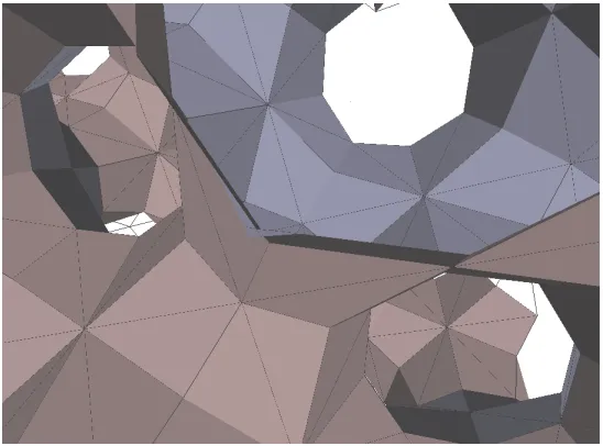
This algorithm was implemented for simple cubic and a surface resembling the p surface was produced. The code can be seen in the appendix and pictures seen in figures 4.1 and 4.2.

4.4 Intersections

There is still another problem to consider here, namely, how would we go about determining whether there are any intersections between triangles in our trian-gulated surface.

(39)

[image:39.612.185.408.127.374.2]

Figure 4.1: The final surface computed for simple cubic.

[image:39.612.142.416.440.643.2]

(40)

Our idea to make this easier is to represent our potential embedding as a homomorphism acting on the Coexter group. First we introduce the following notation.

Definition 4.8.

(c,(σik)k∈{0,...,n}) = (c, σi1)(σi1c, σi2)...(c, σin) (4.2)

Consider then that in our algorithm we fix a starting vertex on the Delaney-Dress graph. Let our starting vertex be c. We then assign all vertices, c’ on the Delaney-Dress graph a path xc0. All of these paths start at c, and hence using

the above notation can be represented as (c,(σik)k∈{0,...,n}) or simply in the

form (σik)k∈{0,...,n}). We might then be tempted to identify this form directly

with the Coexter group, but we immediately have to be careful due to the fact the that we created an abelian group over these (c, σi) elements.

To deal with this we note the following.

Theorem 4.9. Every simple path has a unique representation in the form

(c, σikk∈{0,...,n}), where((c, σik))k∈{0,...,n} is a path.

Proof We first imagine a simple path as an element of the first-order chain group of the Delaney-Dress graph. This is in an abelian group so we can order the generators however we wish. This ordering is a path ordering if for ei = (c0, σi) we have that o(ei) = t(ei−1). We then choose this ordering for the generators. Note then that because this path is simple ifo(ei) =o(ej), then i = j and hence there is only one way to form this ordering and this gives us a unique representation.

Since the algorithm is independent of choice of path we can then choose sim-ple paths for all vertices. We can then represent the Delaney-Dress embedding as a homomorphism on the Delaney-Dress graph to a collection of vectors in

(41)

A= {2, 25, 5, 7, 9, 11, 13, 15, 17, 19, 21, 23, 44, 27, 29, 31,

33, 35, 37, 39, 41, 43, 46, 48, 50, 52, 54, 56, 58, 60, 62, 64, 66, 68, 70, 72, 74, 76, 78, 80, 82, 84, 86, 88, 90, 92, 94, 96};

B = {3, 96, 6, 78, 76, 10, 35, 32, 14, 86, 83, 18, 66, 64, 22, 46,

24, 26, 95, 30, 54, 51, 34, 38, 62, 59, 42, 90, 88, 45, 49, 74, 72, 53, 57, 82, 79, 61, 65, 69, 94, 92, 73, 77, 81, 85, 89, 93};

F = {4, 5, 22, 8, 9, 12, 13, 16, 17, 20, 21, 25, 43, 28, 29, 32,

33, 36, 37, 40, 41, 44, 47, 48, 51, 52, 55, 56, 59, 60, 63, 64, 67, 68, 71, 72, 75, 76, 79, 80, 83, 84, 87, 88, 91, 92, 95, 96}

ThisstoresthecompressedformoftheDelaney-Dresssymbol.

G := {}; n := 1;

While[ n < 97, If[! MemberQ[A, n], AppendTo[G, n]]; n++]

H := {}; n :=1; While[n < 97, If[!MemberQ[B, n], AppendTo[H, n]];

n++]

J := {}; n :=1; While[n<97, If[!MemberQ[F, n], AppendTo[J, n]]; n++]

Thesegeneratethemissingnumbersfromthecompressedformintheappropriateorder.

K := {}; n := 1;

While[n < 97, If[MemberQ[A, n], AppendTo[K, G[[FirstPosition[A, n]]]],

AppendTo[K, A[[FirstPosition[G, n]]]]]; n++]; m := 1; While[m < 97,

If[MemberQ[B, m], AppendTo[K[[m]], First[H[[FirstPosition[B, m]]]]],

AppendTo[K[[m]], First[B[[FirstPosition[H, m]]]]]]; m++];

k := 1; While[k < 97, If[MemberQ[F, k],

AppendTo[K[[k]], First[J[[FirstPosition[F, k]]]]],

AppendTo[K[[k]], First[F[[FirstPosition[J, k]]]]]]; k++]

ThisdeterminetheuncompressedformoftheDelaney-Dresssymbolbycomparingelementsfrom theprevioustwoliststodetermineadjacencies.

L := {}; n :=1; While[n<97, AppendTo[L, 0]; n++]

M := {};

m :=1;

P := {};

While[m<4, AppendTo[P,{}];

n :=1;

While[n<97, If[K[[n]][[m]] >n,

AppendTo[M, ReplacePart[ReplacePart[L, n→-1 ], K[[n]][[m]]→1]];

AppendTo[P[[m]],{n, K[[n]][[m]]}]];

n++];

m++];

Q :=Transpose[M]

Thisgeneratesathefirst-orderboundarymapoftheDelaney-Dressgraphaswellasanorderingon theedgesasareferenceforthechoiceofbasisinallfuturematrixcalculations.

R :=NullSpace[Q]

(42)

ThiscalculatesthehomologygroupoftheDelaney-Dressgraph.

S := {};

n :=1;

m :=1; While[n<13, While[m<97, If[!MemberQ[S, m, 2], k :=1;

AppendTo[S,{m}];

While[k<8, AppendTo[S[[n]], P[[If[Mod[k, 2]⩵1, 1, 2]]][[FirstPosition[

P[[If[Mod[k, 2]⩵1, 1, 2]]], S[[n]][[k]]][[1]]]][[If[FirstPosition[

P[[If[Mod[k, 2]⩵1, 1, 2]]], S[[n]][[k]]][[2]]⩵1, 2, 1]]]];

k++]n++];

m++]]

T := {};

n :=1;

m :=1; While[n<9, While[m<97, If[!MemberQ[T, m, 2], k :=1;

AppendTo[T,{m}];

While[k<12, AppendTo[T[[n]], P[[If[Mod[k, 2]⩵1, 2, 3]]][[FirstPosition[

P[[If[Mod[k, 2]⩵1, 2, 3]]], T[[n]][[k]]][[1]]]][[If[FirstPosition[

P[[If[Mod[k, 2]⩵1, 2, 3]]], T[[n]][[k]]][[2]]⩵1, 2, 1]]]];

k++]n++];

m++]]

U := {};

n :=1;

m :=1; While[n<25, While[m<97, If[!MemberQ[U, m, 2], k :=1;

AppendTo[U,{m}];

While[k<4, AppendTo[U[[n]], P[[If[Mod[k, 2]⩵1, 3, 1]]][[FirstPosition[

P[[If[Mod[k, 2]⩵1, 3, 1]]], U[[n]][[k]]][[1]]]][[If[FirstPosition[

P[[If[Mod[k, 2]⩵1, 3, 1]]], U[[n]][[k]]][[2]]⩵1, 2, 1]]]];

k++]n++];

m++]]

Thesegeneratelistsofvertex,edgeandfaceorbits,inotherwordsthealternatingcolourloops.For futurereference.

L1 := {}; n :=1; While[n<145, AppendTo[L1, 0]; n++]

V := {}; n :=1;

Whilen<13, m :=1; AppendTo[V,{}]; Whilem<9, AppendToV[[n]],

ReplacePartL1,FirstPosition[P[[If[Mod[m, 2]⩵1, 1, 2]]], S[[n]][[m]]][[

1]] +If[Mod[m, 2]⩵1, 0, 48] → If[FirstPosition[

P[[If[Mod[m, 2]⩵1, 1, 2]]], S[[n]][[m]]][[2]]⩵1, 1, -1];

m++;

n++

V1 := Total[V,{2}]

2�� Thesis.nb

(43)

W := {}; n :=1; Whilen<9, m :=1;

AppendTo[W,{}];

Whilem<13, AppendToW[[n]], ReplacePartL1,FirstPosition[P[[If[Mod[m, 2]⩵

1, 2, 3]]], T[[n]][[m]]][[1]] +If[Mod[m, 2]⩵1, 48, 96] → If[

FirstPosition[P[[If[Mod[m, 2]⩵1, 2, 3]]], T[[n]][[m]]][[2]]⩵1, 1,-1];

m++;

n++

W1 :=Total[W,{2}]

X := {};

n :=1;

Whilen<25, m :=1;

AppendTo[X,{}];

Whilem<5, AppendToX[[n]], ReplacePartL1,FirstPosition[P[[If[Mod[m, 2]⩵1,

3, 1]]], U[[n]][[m]]][[1]] +If[Mod[m, 2]⩵1, 96, 0] → If[

FirstPosition[P[[If[Mod[m, 2]⩵1, 3, 1]]], U[[n]][[m]]][[2]]⩵1, 1,-1];

m++;

n++

X1 :=Total[X,{2}]

Thesegeneratevectorsinthefirst-orderhomologygroupwithrealcoeﬀicientscorrespondingto thealternatingcolourloops.Theseareusedbutwereultimatelyfoundtoberedundant.

Y= Join[V1, W1, X1, R]

Thiscreatesalistofvectorsthatspanthefirst-orderhomologygroup,madeupof,firstthevectors computedinthelastpart,andthenthebasisvectorscomputedbeforefromtheboundarymap.

Z= Orthogonalize[Y]

AA := {};

n :=1; Whilen<94, If!Z[[n]]⩵L1, AppendTo[AA, Z[[n]]];

n++

ThisappliesGram-Schidmttothepreviouslistofvectorsandthenremovesthezerovectors pro-duced.Thebenefitisthatwiththisbasisweknowthefirst‘x’numberofvectorscorrespondtothe subspacespannedbythealternatingcolouredloops.Soifwethenselectalloftheothervectorswe willhaveabasisforaspaceperpendiculartothiscolouredsubspace.Thisisusefulsincethe colouredsubspaceiscontainedinHandhenceallowsusnotinsteadofprojectingontothe first-orderhomologygroupwecanprojectontoasubspacethatisclosertothefinalspacewewishto projectto.Unfortunatelythisturnedouttonotsaveanytimewhatsoeverandwascompletely useless.Butitdidn’thurtsoohwell.

AB := {}; n :=1; While[n<7, AppendTo[AB, AA[[50-n]]]; n++]

AC=Transpose[AB].AB

Thesecollectthevectorscorrespondingtothesubspacewewishtoprojecttoandcomputesthe projectionmap.

Thesis.nb ��3

Crystallographic Surfaces

Crystallographic Surfaces

Contents

Dedication

Where don’t we find

crystals?

Chapter 1

Motivation

1.1

The Adventures of Agnes, Barry and Clara,

Episode I

1.2

What is a crystal?

1.3

How do we find crystals?

1.4

Are all crystals surfaces?

Chapter 2

Sunada’s Method

2.1

The Adventures of Agnes, Barry and Clara,

Episode II

2.2

Combinatorial Graphs

2.3

Enumerating Crystals with Covering Space

Theory

2.4

Sunada’s Algorithm

Chapter 3

Crystallographic Surfaces

3.1

The Adventures of Agatha, Barry and Clara,

Episode III

3.2

Crystallographic Surfaces

3.3

Enumerating Crystallographic Surfaces

Chapter 4

Inverting EPINET

4.1

The Adventures of Agatha, Barry and Clara,

Episode IV

4.2

Surfaces from Crystals

4.3

A Worked Example

4.4

Intersections