Using conditional kernel density estimation for wind power density forecasting

Using Conditional Kernel Density Estimation

for Wind Power Density Forecasting

Jooyoung Jeon*

Strathclyde Business School, University of Strathclyde

James W. Taylor

Saïd Business School, University of Oxford

Journal of the American Statistical Association, forthcoming

*

Address for Correspondence:

Jooyoung Jeon

Department of Management Science University of Strathclyde

Graham Hills Building, 40 George Street GLASGOW G1 1QE, UK

Tel: +44 (0)141 548 3141 Fax: +44 (0)141 552 6686

Abstract

Of the various renewable energy resources, wind power is widely recognized as one of

the most promising. The management of wind farms and electricity systems can benefit

greatly from the availability of estimates of the probability distribution of wind power

generation. However, most research has focused on point forecasting of wind power. In

this paper, we develop an approach to producing density forecasts for the wind power

generated at individual wind farms. Our interest is in intraday data and prediction from 1

to 72 hours ahead. We model wind power in terms of wind speed and wind direction. In

this framework, there are two key uncertainties. First, there is the inherent uncertainty in

wind speed and direction, and we model this using a bivariate VARMA-GARCH (vector

autoregressive moving average-generalized autoregressive conditional heteroscedastic)

model, with a Student t distribution, in the Cartesian space of wind speed and direction. Second, there is the stochastic nature of the relationship of wind power to wind speed

(described by the power curve), and to wind direction. We model this using conditional

kernel density (CKD) estimation, which enables a nonparametric modeling of the

conditional density of wind power. Using Monte Carlo simulation of the

VARMA-GARCH model and CKD estimation, density forecasts of wind speed and direction are

converted to wind power density forecasts. Our work is novel in several respects:

previous wind power studies have not modeled a stochastic power curve; to

accommodate time evolution in the power curve, we incorporate a time decay factor

within the CKD method; and the CKD method is conditional on a density, rather than a

single value. The new approach is evaluated using datasets from four Greek wind farms.

Key words: Wind energy; Predictive distribution; Kernel estimation; Wind speed; Wind

1. INTRODUCTION

Wind power is the fastest growing form of renewable energy. Efficient

management of wind farms and electricity systems requires forecasts of the power

generated. This is a challenging forecasting task due to the erratic nature of wind and the

nonlinear relationship between the variables involved. In an effort to enhance the

information provided by the forecasters, probabilistic forecasting has been a recent area

of development in wind energy forecasting (Bremnes 2004; Pinson and Kariniotakis

2010). The extension from deterministic forecasting to probabilistic allows more efficient

management of the transmission system through improved load dispatch and better

scheduling of spinning reserve. For a wind farm operator, a probabilistic forecast enables

improved decision making regarding the amount of energy to commit to the electricity

grid for a future period, which is important given the financial penalties that are incurred

for the shortfall. Ultimately, a probabilistic assessment of the uncertainty in wind energy

generation will bring societal benefits by enabling more efficient energy management

resulting in a reduced reliance on power generation from fossil fuels.

Although there has been substantial attention paid by researchers to methods for

wind power point forecasting, methods for wind power density forecasting are far less

developed. One approach to density forecasting would be to fit a univariate statistical

model to the wind power time series, but this is not straightforward due to the inherent

nonlinear evolution of wind power. The alternative is to convert wind speed density

forecasts to wind power density forecasts using the power curve, which relates wind

power to wind speed. This approach is the focus of this paper. It relies on the availability

Gneiting et al. 2006; Taylor et al. 2009; Sloughter et al. 2010; Gneiting 2011a). As for the

power curve, historical data indicates that there is substantial variability in the

relationship between wind speed and wind power (S nchez 2006). It would seem wise to

take this additional uncertainty into consideration when converting wind speed density

forecasts to wind power density predictions.

This paper is the first to produce wind power density forecasts by explicitly

modeling both the wind speed uncertainty and the stochastic power curve. With our focus

on hourly data and relatively short forecast lead times, we use a time series model for

wind speed density forecasting, rather than ensemble predictions from an atmospheric

model. Advantages of using time series models are: (i) they are no less accurate than

atmospheric modeling for short-term predictions (Focken et al. 2002); (ii) they can

produce forecasts from any time origin and for any lead time, which contrasts with

atmospheric model ensemble predictions (see, for example, Taylor et al., 2009); (iii)

acquiring forecasts from an atmospheric model can be costly; and (iv) predictions from

such models are often not available for the wind farm location of interest. Following the

work of Cripps and Dunsmuir (2003) and Hering and Genton (2010), we use a bivariate

VARMA-GARCH (vector autoregressive moving average-generalized autoregressive

conditional heteroscedastic) time series model, which enhances wind speed prediction

through the joint modeling of wind speed and direction. We convert the resulting wind

speed density predictions into wind power density forecasts using Monte Carlo

simulation and conditional kernel density (CKD) estimation (see Rosenblatt 1969;

Hyndman et al. 1996), which enables a nonparametric modeling of the conditional

density of wind power. The method involves kernel weighting over the conditioning

Our use of CKD estimation has two novel features: (i) the CKD estimation is conditional

on a density, rather than a single value, and (ii) to model time evolution in the

relationship between wind power and the conditioning variables, we incorporate a time

decay factor within CKD estimation.

To illustrate implementation of our approach, and to compare it to alternatives, we

use data from four Greek wind farms, and evaluate forecast accuracy from 1 to 72 hours

ahead. Due to the intermittency and non-dispatchable nature of wind energy, accurate

short-term wind power forecasts from 15 minutes up to several days ahead are vital to

transmission system operators, who maintain the balance between load and generation.

For wind farm operators, the accuracy of short-term wind power forecasts is crucial for

minimizing the penalties for failing to meet the commitment. Very short-term forecast

horizons from a few seconds to an hour are related to turbine active control in wind farms.

Long-term horizons up to 7 days are useful for maintenance planning of wind turbines.

Section 2 presents the Greek wind power dataset. Section 3 describes the

VARMA-GARCH model that we use to produce wind speed and direction density

forecasts. Section 4 explores the stochastic nature of the relationship between these two

variables and wind power. Section 5 introduces CKD estimation, and Section 6 describes

our use of CKD estimation for wind power density forecasting. Section 7 presents

empirical results, and Section 8 provides a brief summary and conclusion.

2. THE WIND DATA

For the empirical work in this paper, we used hourly data from four wind farms in

Crete: Aeolos, Rokas, Enteka and Iweco. Crete is the largest island in the Aegean Sea. It

Aeolos, Enteka and Rokas, which are in the east of Crete, consist of data from January 1,

2006 to December 31, 2006, which amounts to 8,760 hourly observations. The data from

Iweco wind farm, which is located in the center of Crete, is over a shorter period from

January 1, 2006 to October 30, 2006, which amounts to 7,272 observations. The wind

speed, direction and power data were provided rounded to the nearest 0.1 m/s, 0.1° and

0.1 MW, respectively. For each wind farm, the wind speed and direction were recorded at

a meteorological tower near to the wind farm at the hub height of the wind farm‟s

turbines. The wind power data corresponds to total power generated from the whole wind

farm. The capacities of the Aeolos, Enteka, Iweco and Rokas wind farms, at the end of

2006, were 11.6 MW, 2.8 MW, and 4.3 MW and 16.3 MW, respectively. In our empirical

forecasting comparison of Section 7, the last 25% of each wind power series is used as

the post-sample period. Figure 1 shows the time series plots for wind speed, direction and

power for the Aeolos wind farm. All three series exhibit substantial variability. The wind

power series is bounded above by the capacity of the wind farm. Interestingly, the wind

power plot seems to indicate shifts in the capacity during January and February, and in

the first half of July. The rise in the capacity around the end of February was due to new

turbine installations, but we do not have explanations for the other apparent capacity

changes. In Sections 3 and 4, we provide further descriptive plots to gain insight into the

three wind variables and the relationships between them.

3. BIVARIATE VARMA-GARCH MODEL FOR WIND SPEED AND DIRECTION

In fitting a statistical model to wind speed time series, it has been suggested that

wind direction can enhance the model, and hence improve wind speed forecast accuracy.

Harbor, Cripps and Dunsmuir (2003) transform the minute-by-minute time series of wind

speed and direction to Cartesian coordinates, and model the pair of wind velocity

variables using a bivariate vector autoregressive moving average (VARMA) model with

error variances described by a bivariate generalized autoregressive conditional

heteroskedastic (GARCH) process and a Student t distribution for the error terms. Gneiting et al. (2006) identify two distinct forecast regimes, split by wind direction, in

hourly time series of wind speed and direction in the U.S. Pacific Northwest. They

propose spatial and temporal regime switching models using a vector autoregressive idea

and a truncated Gaussian distribution for two-hour ahead prediction. For the same data,

Hering and Genton (2010) consider a univariate wind speed model incorporating wind

direction in trigonometric forms using the truncated Gaussian distribution, and also a

bivariate model for wind speed and direction, in Cartesian coordinate form, using a

skewed t distribution.

A major benefit of modeling wind speed and wind direction, after transformation

to Cartesian coordinates, is that non-negativity of wind speed prediction is automatically

ensured. The two axes of the coordinates represent wind velocities corresponding to the

east-west and north-south wind components. In this paper, we use a bivariate model for Zt

= (Ut,Vt), where Ut = Xtsin(t+), Vt = Xtcos(t+), Xt is the wind speed at time t,t is

the wind direction at time t, and  is a constant parameter that is estimated along with the

model parameters using maximum likelihood. Our inclusion of the parameter  is new. It

is intended to rotate the coordinate axes, so that one of them is aligned with a commonly

right hand side of the figure. The plots indicate that, for this particular wind farm, wind

blows more frequently at approximately 20° (north-easterly) and 250° (south-westerly).

In the model that we use for Aeolos in our empirical analysis of Section 7, the optimized

value of the parameter  was estimated as 30.1°. This implies that the axes are rotated

anticlockwise by 30.1°, which results in the Ut axis approximately aligning with the commonly occurring Aeolos south-westerly wind direction.

We use a similar model to that presented by Cripps and Dunsmuir (2003). Using

the VEC form of the bivariate GARCH model of Bollerslev et al. (1988), we estimated

the entire covariance matrix of VEC, rather than the diagonal covariance matrix assumed

by Cripps and Dunsmuir (2003). The model is given in expressions (1)-(4). Expression

(1) is the VARMA part of the model and expression (3) is the bivariate GARCH part.

, ) , ( 1 1 t r j j t j m i i t i

t  t





 

 

 



s A B Z

Z (1)

,

2 1

t t

t H η

 (2)

, ) ( vech ) ( vech ) , ( ) ( vech 1 1





t t D G H

H sω   (3)













) , ( 1 24 ) ( 2 , 24 ) ( 1 , 0



i i i

t   



s (4)

where Zt is the (2×1) vector of wind velocities; t is a vector of error terms; Ht is the

conditional covariance matrix of t; ηt is an i.i.d. vector of error terms; vech(·) denotes the

column stacking operator of the lower triangular part of the symmetric matrix that is its

argument; Ai and Bj are (2×2) matrices of parameters;Di and Gj are (3×3) matrices of

seasonal terms with (2×1) constant parameter vectors μi; s(ω,t) is a (3×1) vector of

deterministic intraday seasonal terms with (3×1)constant parameter vectors ω_i; N_ is a

non-negative integer indicating the number of terms in the summation of s(γ,t); and h(t)

is a repeating step function that numbers the hours from 1 to 24 within each day.

We used the Schwarz‟s Bayesian Criterion to select the order of the VARMA and

GARCH components of the model, and the N_r. We considered VARMA and GARCH

lags up to order 24, and Nr 8. For our data, we implemented the VARMA-GARCH

model using multivariate Gaussian, Student t and skewed t (Azzalini and Genton 2008)

distributions for t. Table 1 summarizes the three models fitted to the Aeolos wind farm

data. The axes-rotation  parameter is significant for each of the three models. The table

shows that the values of the degrees of freedom were low for the models with Student t and skewed t distributions, suggesting that the distribution is not close to Gaussian. In the table, the orders of the models are reasonably low, especially for the two non-Gaussian

distributions, and it is interesting to see that diurnal seasonality only features in the

Gaussian model. We investigated stationarity by considering, for the ARMA part of the

model, the eigenvalues of the sum of the Ai and Bj matrices, and for the GARCH part, the

eigenvalues of the sum of the Di and Gj matrices (see Fountis and Dickey 1989; Bauwens

et al. 2006). These eigenvalues are shown in the bottom rows of Table 1. Stationarity is

indicated by the eigenvalues being less than one in modulus. The values for the GARCH

part suggest that the model has persistence in its modeling of volatility. When assessed

Recent research has considered how bootstrap procedures can be used to include

parameter uncertainty in density forecasts generated from GARCH models (Reeves 2005;

Pascual et al. 2006). However, such procedures are highly computational as they require

repeated maximum likelihood estimation. Chen et al. (2011) suggest approximating a

GARCH model as a linear process written in terms of squared residuals, which can then

be estimated using least squares. This idea is not readily applicable to the multivariate

GARCH model in this paper. In addition, bootstrapping such a model would seem to be

computationally challenging. In view of this, in producing density forecasts from our

VARMA-GARCH model, we did not account for the parameter estimation uncertainty.

However, this is an aspect of our analysis that could be developed in future work.

4. THE POWER CURVE

Our proposed methodology for wind power density forecasting requires an

understanding of the relationship between wind power and wind speed, which is

described by the power curve. Although wind power theoretically depends on wind speed,

air density and the area swept by the turbine blades, turbine manufacturers typically

provide information regarding the power curve for an individual wind turbine assuming

fixed air density. A power curve has a „cut-in speed‟, at which the turbine blades begin to

rotate; a „rated speed‟, which is the lowest speed at which the maximum power output of

the turbine is generated; and a „cut-out speed‟, beyond which the turbine is shut down to

prevent damage. An idealized deterministic curve, of this form, is used in the work of

Taylor et al. (2009), Hering and Genton (2010) and Gneiting (2011a). However, as these

nche (2006) explains that, in reality, the form of the power curve depends on

meteorological variables such as wind direction, temperature, local air density and

precipitation. He notes that the behavior of power curves when the wind speed increases

can be different from the behavior when the speed decreases. Furthermore, the task is to

predict wind power for an entire wind farm, and for this, the power curve of the whole

wind farm is needed. The choice of a deterministic power curve is then complicated by

the fact that the wind turbines in a wind farm can have different cut-in, rated and cut-out

speeds, and that there may be changes in the power capacity of the wind farm due to the

addition of new turbines and turbine maintenance. Also, apparent changes in the capacity

can be due to down-ramping to reduce the amount of wind energy entering the utility

system. Given the complexity of the power curve, in practice, a deterministic power

curve is often derived from historical wind speed and power data recorded at the wind

farm level.

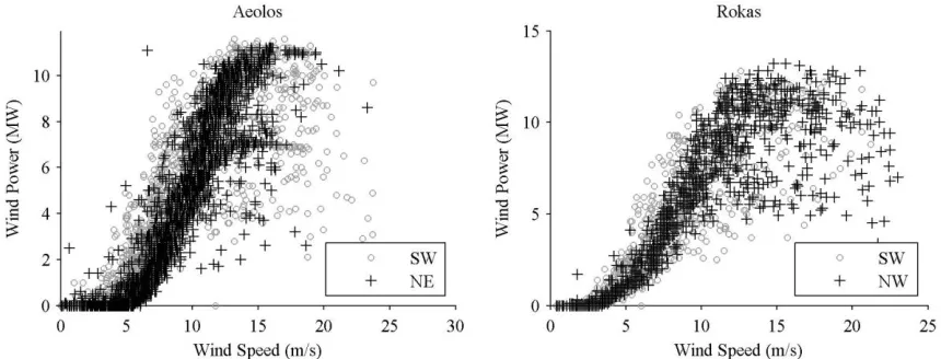
In Figure 3, we plot the historical wind power and wind speed data for two of the

Greek wind farms. The typical features of a power curve are evident, along with

substantial variability. In this paper, our approach to wind power density forecasting aims

to capture the stochastic nature of the power curve. In Figure 4, we again plot wind power

against wind speed, but, in this plot, we use different symbols to show the data points for

selected months. The figure seems to show the wind farms' capacities changing over time.

As noted in Section 2, the capacity of the Aeolos wind farm increased around the end of

February 2006 due to the installation of new turbines. However, we do not have

explanations for the other apparent capacity changes. Unfortunately, information

forecaster. Therefore, our approach to wind power density forecasting should try to

accommodate the potentially time-varying nature of the power curve.

Although wind turbines are able to turn to face the wind, it has been suggested

that the relationship between wind power and wind speed is, to some extent, dependent

on the wind direction. Potter et al. (2007) find that the uncertainty in the relationship

depends on the wind direction. Nielsen et al. (2006) include a wind direction variable into

the relationship to explain turbine wake effects and direction dependent bias of the

meteorological forecasts. nche (2006) recognizes that wind direction influences the

performance of a wind farm, and so uses it in a wind power prediction model. In Figure 5,

we plot wind power against wind speed using different symbols to show the data points

for selected wind directions. The plots suggest that the variability in the relationship can

depend on wind direction. For Aeolos, south-westerly wind seems to produce a higher

degree of variability in the relationship, and for Rokas, south-westerly wind shows higher

variability than north-westerly when the wind speed is below about 13 m/s.

As mentioned in Section 3 for the Aeolos wind farm, wind blows more frequently

around 20° and 250°. The plot on the right hand side of Figure 2 indicates that, in these

directions, the level and variability of the wind speed is lower than from other directions.

This might be due to the inherent characteristics of the wind, or to the terrain surrounding

the wind farm. We investigate the influence of wind direction on the relationship of wind

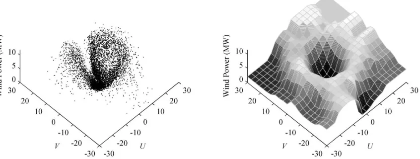
speed and power by plotting power against both speed and direction on the left hand side

of Figure 6. A smooth surface, fitted by the Nadaraya-Watson estimator (see Nadaraya

1964; Watson 1964), is shown on the right hand side of the figure. The surface indicates

that, for speed above about 20 m/s, the wind blowing around 30, 80 and 240 tends to

its relationship to wind speed, and wind speed itself are dependent, to some extent, on

wind direction. This supports our joint modeling of wind speed and direction in Section 3,

and motivates the inclusion of wind direction in our modeling of wind power.

The conversion of a wind speed density forecast into a wind power density

forecast is a conditional density estimation problem. If the conditional wind power

density were to follow a Gaussian distribution with a constant variance and a mean that is

a linear function of explanatory variables, it would be a standard multiple regression

problem. However, the relationship between wind power and wind speed is nonlinear,

and the conditional density of wind power is often skewed and can be bimodal, and,

importantly, its shape is conditional on the value of the wind speed. This dependence on

wind speed is illustrated by Figure 7, which shows smoothed histograms of wind power

for different values of wind speed. In this paper, we use conditional kernel density

estimation to overcome the issues of nonlinearity and a non-Gaussian conditional density.

5. CKD ESTIMATION

Conditional kernel density (CKD) estimation enables density estimation of a

variable conditional on the value of one or more explanatory variables. The method is

nonparametric in two senses; it involves no parametric assumption for the density of the

target variable, and it makes no parametric assumption regarding the form of the

relationship between target and explanatory variables. This is enabled through the use of

double kernel estimation. Since the method involves no distributional assumption, the

conditional kernel density estimation is particularly advantageous in estimating the

density when the conditional distribution is multimodal or skewed, as is often the case in

dependency of wind power on wind speed, CKD would seem to be very suitable for

estimating wind power densities conditional on values for wind speed.

We define Yt as dependent variable and Xt as explanatory variable. Let f





the conditional density function of Yt given Xt = x. The Rosenblatt CKD estimator (Rosenblatt 1969) of f(y|x) is written as

, ) ( ) ( ) ( ) | ( ˆ 1 1





where n is the sample size, and Kh(·)=K(·/h)/h is a kernel function with bandwidth h. This formulation contains two bandwidths, hx and hy. They are scale parameters that control the amount of smoothing. We discuss our approach to bandwidth optimization in Section

6. An estimate of the full density function can be built up by repeating the CKD

estimation for a range of y values. The CKD estimator involves double kernel estimation, with kernel density estimation in the y direction and kernel smoothing in the x direction. For a given x, the density function of Yt at the value y is constructed by applying kernel density estimation to the sample of values of Yt, with each Yt value weighted in accordance with the proximity of the corresponding Xt relative to the value x.

Hyndman et al. (1996) note that the mean of the Rosenblatt estimator is a biased

estimator of the conditional mean. To address this, they propose a two-step CKD

estimator. In the first step, the conditional mean is estimated using some form of unbiased

kernel smoothing. Subtracting the resulting mean estimates from the observed values for

Yt delivers a set of residuals et. In the second step, the Rosenblatt CKD estimator is applied to these residuals. The Hyndman et al. two-step CKD estimator is given in

, ) ( ) ˆ ( ) ( ) | ( ˆ 1 1





where eˆ_t Y_tmˆ(X_t) and eymˆ(x) (7)

This formulation contains the bandwidths, hx and he, and possibly additional bandwidths associated with the estimation of the conditional mean. As with the

Rosenblatt CKD estimator, an estimate of the full density function can be produced by

repeating the Hyndman et al. CKD estimation for different values of y.

There are not many examples of the use of CKD estimation in a time series

context. Hyndman et al. use their density estimator for daily temperature conditional on

lagged temperature and a seasonal variable. Bashtannyk and Hyndman (2001) use the

estimator for the density of the eruption duration of the Old Faithful geyser conditional

on waiting time. Fan and Yim (2004) extend the Rosenblatt estimator using a local linear

regression, and forecast the density of the yield change of treasury bills conditional on the

current yield. Juban et al. (2007) use the Rosenblatt CKD estimator to predict wind power

densities conditional on the most recent wind power observation and point forecasts of

wind speed and direction produced by an atmospheric model. Our use of CKD differs

from this in that we produce wind power density forecasts conditional on density

forecasts of wind speed and direction.

6. A NEW APPROACH TO CKD ESTIMATION FOR WIND POWER MODELING

6.1. CKD Estimation Conditional on Wind Speed

For wind power density forecasting, we implemented the two-step CKD estimator

and speed, respectively. We considered the Loess mean estimator of Cleveland (1979)

and the Nadaraya-Watson mean estimator. However, the two-step CKD estimator led to

wind power density forecasts that were only slightly more accurate than those produced

by the Rosenblatt CKD estimator of expression (5). In view of this, we felt we could not

justify the use of the more complex two-step estimator, and so, in this section, we report

the results for the simpler Rosenblatt CKD estimator.

In our work, the full wind power density function was constructed by repeating

the CKD estimation for values of y from ero to the wind farm‟s capacity with increments equal to 1% of the capacity. Linear interpolation between the resulting values of the

density function delivered an estimate of the complete wind power density. Using a finer

increment than 1% of the capacity led to increased computational burden with very little

improvement in density forecast accuracy. We used a Gaussian kernel. We also tested a

truncated Gaussian kernel, since the wind power is a bounded variable, but we found no

practical benefit, which is consistent with the comments of Hyndman and Yao (2002).

The CKD estimator enables the density function of wind power to be estimated

for a given value of the explanatory variable, wind speed. However, for any future period,

the value of wind speed is of course unknown. Indeed, the purpose of the

VARMA-GARCH model of Section 3 is to produce wind speed density forecasts. We are not aware

of any previous studies that have considered the application of the CKD estimator when

the explanatory variable is stochastic. In this paper, we introduce a CKD-based approach

to estimating the wind power density conditional on a density for the explanatory variable, wind speed. The approach involves the following three stages:

(1) The CKD estimator is used to produce an estimate of the full wind power

of 0.1 m/s. The result is 301 different wind speed values and their corresponding

conditional wind power density estimates, which are stored for use in Stage 2.

(2) Monte Carlo simulation of the bivariate VARMA-GARCH model of Section 3

is performed to generate 1,000 realizations of wind speed for a selected lead time. These

1,000 values can be considered as sampled values from the model‟s wind speed density

forecast. We rounded to the nearest 0.1 m/s each of the 1,000 wind speed simulated

values, and then obtained the corresponding conditional wind power density estimates,

which had been stored in Stage 1.

(3) The 1,000 wind power density estimates from Stage 2 are averaged to give a

single wind power density forecast.

In the approach, 30 m/s was chosen, as it was perceived as being the maximum

possible wind speed. We considered finer increments than 0.1 m/s, but this led to

increased computational cost, without noticeably improving density forecast accuracy.

With regard to bandwidth selection for CKD estimation, the literature can be

divided into two categories, namely a rule-based approach (Hall et al. 1999; Bashtannyk

and Hyndman 2001; Hyndman and Yao 2002) and a data-driven approach (Fan and Yim

2004; Hall et al. 2004). Hall et al. (2004) comment that there is no general rule for the

optimal bandwidth parameter, and that cross-validation delivers more appropriate

bandwidths, particularly when multiple explanatory variables are involved, such as in

Section 6.2, where we use wind speed and direction. Fan and Yim (2004) find that

cross-validation outperforms rule-based approaches. Holmes et al. (2007) write that rule-based

approaches tend to perform poorly in finite samples when the reference distribution is not

In the cross-validation, we selected the kernel bandwidths that led to the most

accurate wind power density estimates, conditional on observed wind speed, where

accuracy was measured by the mean continuous ranked probability score (CRPS)

calculated over the cross-validation evaluation period for one hour ahead prediction. The

CRPS captures the two important characteristics of a density forecast: its location relative

to the observed value and its sharpness around that value (see Gneiting et al. 2007).

For the kernel density estimation methods, we used a rolling window of six

months. This amounted to 50% of the length of the entire dataset. The penultimate 25%

of the dataset was used as the cross-validation evaluation period, and the last 25% of the

dataset was used for post-sample evaluation of the wind power density forecasts. The

bivariate VARMA-GARCH model was estimated using the first 75% of the data.

Elsewhere in the paper, we refer to this as the „in-sample‟ period of data.

We used a fixed length rolling window in the kernel density estimation methods

because the optimized bandwidths tended to vary with the length of the rolling window,

with the bandwidths tending to be larger for shorter windows. The six-month rolling

window was not updated every forecast origin, but updated every 24 hours in order to

reduce computational running time. We experimented with rolling window lengths of

three months and one month, and found that the resultant wind power density forecast

accuracy was very similar to that for the six-month window. However, this was not the

case when conditioning CKD estimation on wind speed and wind direction, which is

described in the next section. For this, we found that density forecast accuracy for

Hyndman et al. (1996) suggest the use of different bandwidths for different values

of the explanatory variable x. We experimented with a different value of hx for different ranges of wind speed values. However, this did not lead to a clear benefit in accuracy.

6.2. CKD Estimation Conditional on Wind Speed and Wind Direction

In Section 2, we discussed how the relationship between wind power and wind

speed can vary with wind direction. Therefore, it seems sensible to consider the use of a

wind power CKD estimator with conditioning on both wind speed and direction. As we

discussed briefly in Section 5, Hyndman et al. (1996) and Juban et al. (2007) provide

applications of CKD estimation with more than one explanatory variable. In our

application, we use the transformation to Cartesian coordinates discussed in Section 3,

and condition wind power density estimation on the wind velocities Ut and Vt. In Figure 8, using the in-sample data, we plot the historical relationship between wind power and the

two velocities. In expression (8), we present the Rosenblatt CKD estimator for wind

power conditional on Ut and Vt.

. ) ( ) ( ) ( ) ( ) ( ) , | ( ~ 1 1





This estimator involves two bandwidths, huv and hy. We obtained slightly improved wind power density forecast accuracy when using different bandwidths for the

kernels in the u and v directions. However, as the improvement was not substantial, for the sake of simplicity, in this paper, we treat these bandwidths as being identical.

We implemented the three-stage CKD-based approach described in Section 6.1.

with an increment of 0.5 m/s. We used the larger increment to compensate for the

additional computational cost due to the increased dimension size. (Using an increment of

0.1 m/s did not lead to noticeable improvement in wind power density forecast accuracy.)

6.3. CKD Estimation with Time Decay

The relationship between wind power and the explanatory variables, wind speed

and direction, can evolve over time, as discussed in Section 4 and suggested by Figure 4.

One way of addressing the time-variation is to use only recent information. This could be

enabled by basing estimation on a rolling window. An alternative, which uses all

historical data, is to employ a time decay factor. After observing that the power curve

changes over time, nche (2006) employs a time decay factor within a recursive least

square technique for estimating the time-varying parameters of a model to be used for

wind power point forecasting. In expression (9), we present the Rosenblatt CKD

estimator of expression (5) with an exponential time decay parameter  (0<≤1).

. ) ( ) ( ) ( ) | ( ~ 1 1





A lower value of  implies faster exponential decay, and hence more weight is

given to the recent observations. This allows for a power curve that evolves due to factors

that cannot be modeled explicitly in the CKD estimation framework. We optimized ,

along with the bandwidths, using cross-validation. We also considered the use of the time

7. EMPIRICAL COMPARISON OF POST-SAMPLE FORECAST ACCURACY

We compared the accuracy of wind power density forecasts from the CKD-based

approach with the accuracy of simpler and more traditional methods. As stated previously,

we used the last 25% of each of the four wind power series for post-sample forecast

evaluation. We considered forecasts from 1 to 72 hours ahead. For each wind power

series, we rolled the forecast origin forward (one hour at a time) through the post-sample

evaluation period to produce a collection of forecasts from each method for each horizon.

7.1. Methods

We implemented three different categories of density forecasting methods:

1. Simple kernel density estimation – As a relatively simple benchmark method,

we applied kernel density estimation to a moving window of recent historical wind power

observations. This relatively simple estimator is written as

. ) ( )

| ( ˆ

1



  



 n

l n t

t

h Y y

K x

y f

y

We considered three versions of the method using the following different lengths,

l, for the moving window: (i) 24 hours, (ii) 10 days and (iii) 6 months.

2. Conditioning on wind speed – We implemented the following three methods

that produced wind power density forecasts conditional on just the wind speed variable:

(i) Deterministic with wind speed – The power curve is assumed to be

deterministic, and is estimated using the Nadaraya-Watson estimator for the conditional

mean. Based on this deterministic power curve, wind speed density forecasts are

converted, using Monte Carlo simulation, into wind power density forecasts. This

the uncertainty due to the power curve. This is a relatively sophisticated benchmark

against which to compare the CKD-based methods.

(ii) CKD with wind speed – This is the three-stage method of Section 6.1 based

on the CKD estimator of expression (5).

(iii) CKD with wind speed – This is the three-stage method of Section 6.1 based

on the CKD estimator with exponential decay of expression (9).

3. Conditioning on wind velocities – We implemented the three methods just

described with conditioning on wind speed replaced by conditioning on the two wind

velocities, Ut and Vt. For these three methods, Table 2 presents the bandwidths and

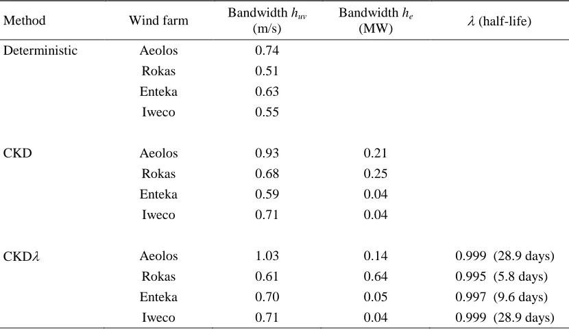
exponential weights optimized using cross-validation. Four of the bandwidths for CKD

are larger than the corresponding bandwidths for CKD, and the opposite is true for two of

the bandwidths. We would suggest larger bandwidths for CKD is intuitive because

exponential decay leads to less historical information being captured, and so there is a

need for a greater degree of kernel smoothing, and this is manifested in larger values for

the bandwidths. This effect was observed by Taylor (2008) for an exponentially weighted

kernel quantile estimator.

To gain insight into the density forecasts produced by the various methods, in

Figure 9, we plot the forecasts of the cumulative distribution function (cdf) produced for

Aeolos and Rokas with forecast origin set as the final period in the in-sample set of data.

We would expect the cdf forecasts from the CKD-based methods to be wider than those

from a method based on a deterministic power curve, because the CKD-based methods

involve the modeling of an additional uncertainty, namely the stochastic power curve.

This is far more apparent in the plot for the Rokas wind farm than the one for Aeolos.

wide, with the effect that this uncertainty substantially dominated the uncertainty due to

the power curve. For Rokas, the cdf forecast from the CKD method is noticeably

different to that from the other CKD-based method. This is not the case for Aeolos, and

this is because the value of the CKD method exponential time decay parameter is 0.999,

which is relatively high, implying slow decay, while the value for Rokas is 0.995.

7.2. Point Forecasting

Although our main focus is density forecasting, we also evaluate point forecast

accuracy, as this provides insight into the accuracy of the central locations of the density

forecasts. We evaluated point forecasts using the mean absolute error (MAE) and the root

mean squared error (RMSE). Gneiting (2011a,b) notes that the median of a density

forecast is the optimal point forecast if the loss function is symmetric piecewise linear,

and the mean is the optimal point forecast for a quadratic loss function. In view of this,

we used the MAE for point forecasts produced as the medians of the density forecasts,

and the RMSE for point forecasts produced as the means of the density forecasts.

For each of the four Greek datasets, and for each method, we calculated the MAE

and RMSE of point forecasts for each forecast horizon from 1 to 72 hours ahead. Table 3

presents the MAE, averaged over the four wind farms, for various lead times and groups

of lead times. We report accuracy for the earlier lead times in more detail because it

seems likely that statistical methods will have more to offer over atmospheric models for

short lead times. The final column of the table summarizes accuracy across all 72 lead

times. In the table, the bold font indicates the best performing method at each lead time.

For the RMSE, the rankings of the methods were very similar to those for the MAE, and

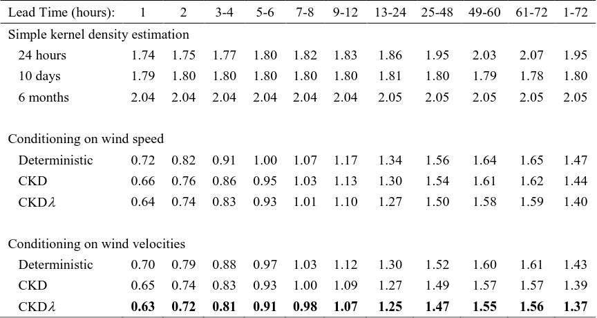
Table 3 shows that the three simple kernel density estimation methods performed

relatively poorly in terms of point forecast accuracy. All three versions of the method

were comfortably outperformed by the other methods at all lead times. Turning to the

three methods that produce forecasts conditional on wind speed, Table 3 shows that the

three produced fairly similar results, with the CKD-based method with exponential time

decay being a little more accurate than the other two methods. It is interesting to note that

each of these three methods, conditional on just wind speed, is outperformed at all lead

times by the corresponding method that produces forecasts conditional on the two wind

velocity variables.

7.3. Density Forecasting

To evaluate density forecast accuracy at each lead time, we calculated the CRPS

averaged across the four wind farms. In Table 4, we summarize these results using the

same format as in Table 3 for point forecasting. As with the point forecasting, the three

simple kernel density estimation methods performed relatively poorly in terms of density

forecasting. Also consistent with the point forecasting results is the superiority of each

method conditional on wind velocities when compared with the corresponding method

conditional on just wind speed. It would seem that wind power density forecast accuracy

does benefit by modeling wind power in terms of both wind speed and direction.

If we focus on the three methods that are conditional on wind velocities, we see

from Table 4 that the two CKD-based methods outperform the method that assumed a

deterministic power curve. The same comment can be made regarding the three methods

conditional on just wind speed. Comparing the methods based on CKD, we can see that

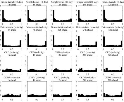
Figure 10 provides further post-sample evaluation of the density forecasting

methods by showing histogram plots of the probability integral transform (PIT) (see

Diebold et al. 1998; Gneiting et al. 2007). We show the PIT values for lead times of 1, 4,

12, 24 and 72 hours, and for four methods: the simple kernel density estimation method

using a 10-day moving window, and the three methods conditional on the wind velocities.

The histograms correspond to the PIT values for all four Greek wind farms. The optimal

shape of a PIT histogram is a uniform distribution. The simple kernel estimation method

and the method based on the deterministic power curve show a high peak in both tails,

demonstrating that their density forecasts are too narrow, underestimating the tail risk.

The histogram plots for the two CKD-based methods are closer to uniform distributions.

7.4. Quantile Forecasting

Interest often lies in the accurate estimation of tail quantiles or a certain prediction

interval. For example, the estimation of tail quantiles provides useful information to

support trading based on future production (Pinson et al. 2007). Furthermore, Gneiting

(2011a) and Pinson et al. (2007) show that a quantile forecast, other than the mean or

median, can be the optimal point forecast in situations where there is an asymmetric cost

function.

To evaluate the quantile forecasts, we use the hit percentage. This measure

assesses the unconditional coverage of a  conditional quantile estimator. It is the

percentage of observations falling below the estimator. Ideally, the percentage should be

. The measure can be viewed as complimenting the CRPS and PIT in evaluating the

density forecasts. For all the density forecasting methods, we obtained the hit percentage

value of 5%. Averaging this value across the four Greek wind farm datasets delivered the

values reported in Table 5. As with point forecast evaluation, smaller values of this mean

absolute error measure are better. Table 6 reports the analogous measure for the

evaluation of forecasts of the 95% quantile.

Looking first at the results for the simple kernel density estimation methods, we

see that the methods performed relatively poorly for the 5% quantile, but for the 95%

quantile, the version of the method based on a moving window of 10 days was more

competitive. It is interesting to see that all the CKD-based methods clearly outperformed

the deterministic power curve methods at each lead time for both the 5% and 95%

quantiles.

8. CONCLUSION

In this paper, we have introduced an approach to wind power density forecasting

that captures the uncertainty due to wind speed, as well as the uncertainty due to the

stochastic nature of the power curve. The approach involves Monte Carlo simulation of a

statistical model and CKD estimation. We considered extensions of the approach that

allow for conditioning on both wind speed and direction, and allow the inclusion of

exponential time decay. Post-sample density forecasting results show that the new

approach was able to outperform a simpler version based on a deterministic power curve,

as well as simple benchmark methods.

In terms of future work, it would be interesting to consider additional explanatory

variables, such as temperature and air pressure, and perhaps also weather information at

upwind locations. In this paper, we have used time series models to produce density

these forecasts on ensemble predictions from an atmospheric model. One might anticipate

that this would be particularly advantageous for the longer lead times. If it is only certain

quantiles of the wind power density that are needed (see Pinson et al. 2007), then it may

be beneficial to optimize the CKD bandwidths separately for each quantile of interest,

rather than for the whole density using CRPS. It would also be interesting to consider the

use of the CKD-based approach in this paper for predicting the density of the total wind

power produced from many wind farms. This could be used by an electricity system

operator to make decisions regarding operating reserve. An additional application of the

CKD-based approach would be to generate a density forecast for the electricity load

conditional on density forecasts for various meteorological variables.

ACKNOWLEDGEMENTS

The authors would like to thank Tilmann Gneiting, Amanda S. Hering, Max Little

and Nigel Meade for their helpful comments and suggestions, as well as George Sideratos

of the National Technical University of Athens and the EU SafeWind Project for

providing the Greek wind farm data. We are also grateful for the helpful comments of

two referees.

REFERENCES

Azzalini, A., and Genton, M. G. (2008), "Robust Likelihood Methods Based on the Skew-t and Related Distributions," International Statistical Review, 76, 106-129. Bashtannyk, D. M., and Hyndman, R. J. (2001), "Bandwidth Selection for Kernel

Conditional Density Estimation," Computational Statistics and Data Analysis, 36, 279-298.

Bauwens, L., Laurent, S. and Rombouts, J. V. K. (2006), "Multivariate GARCH Models: A Survey," Journal of Applied Econometrics, 21, 79-109.

Bremnes, J.B. (2004), "Probabilistic Wind Power Forecasts using Local Quantile Regression," Wind Energy, 7, 47-54.

Chen, B., Gel, Y. R., Balakrishna, N. and Abraham, B. (2011), "Computationally Efficient Bootstrap Prediction Intervals for Returns and Volatilites in ARCH and GARCH Processes," Journal of Forecasting, 30, 51-71.

Cleveland, W. S. (1979), "Robust Locally Weighted Regression and Smoothing Scatterplots," Journal of the American Statistical Association, 74, 829-836.

Cripps, E., and Dunsmuir, W. T. M. (2003), "Modelling the Variability of Sydney Harbour Wind Measurements," Journal of Applied Meteorology, 42, 1131-1138. Diebold, F. X., Gunther, T. A., and Tay, A. S. (1998), "Evaluating Density Forecasts with

Applications to Financial Risk Management," International Economic Review, 39, 863–883.

Fan, J., and Yim, T. H. (2004), "A Crossvalidation Method for Estimating Conditional Densities," Biometrika, 91, 819-834.

Focken, U., Lange, M., Mönnich, K., Waldl, H. P., Beyer, H. G., and Luig, A. (2002), "Short-Term Prediction of the Aggregated Power Output of Wind Farms - A Statistical Analysis of the Reduction of the Prediction Error by Spatial Smoothing Effects," Journal of Wind Engineering and Industrial Aerodynamics, 90, 231-246. Fountis, N. G., and Dickey, D. A. (1989), "Testing for a Unit Root Nonstationarity in

Multivariate Autoregressive Time Series," The Annals of Statistics, 17, 419-428. Gneiting, T., Balabdaoui, F., and Raftery, A. E. (2007), "Probabilistic Forecasts,

Calibration and Sharpness," Journal of the Royal Statistical Society. Series B: Statistical Methodology, 69, 243-268.

Gneiting, T., Larson, K., Westrick, K., Genton, M. G., and Aldrich, E. (2006), "Calibrated Probabilistic Forecasting at the Stateline Wind Energy Center: The Regime-Switching Space-Time Method," Journal of the American Statistical Association, 101, 968-979.

Gneiting, T. (2011a), "Quantiles as Optimal Point Forecasts," International Journal of Forecasting, 27, 197-207.

Gneiting, T. (2011b), "Making and Evaluating Point Forecasts," Journal of the American Statistical Association, 106, 746-762.

Hall, P., Racine, J., and Li, Q. (2004), "Cross-Validation and the Estimation of Conditional Probability Densities," Journal of the American Statistical Association, 99, 1015-1026.

Hall, P., Wolff, R. C. L., and Yao, Q. (1999), "Methods for Estimating a Conditional Distribution Function," Journal of the American Statistical Association, 94, 154-163. Hering, A. S., and Genton, M. G. (2010), "Powering Up with Space-Time Wind

Forecasting," Journal of the American Statistical Association, 105, 92-104.

Hyndman, R. J., Bashtannyk, D. M., and Grunwald, G. K. (1996), "Estimating and Visualizing Conditional Densities," Journal of Computational and Graphical Statistics, 5, 315-336.

Hyndman, R. J., and Yao, Q. (2002), "Nonparametric Estimation and Symmetry Tests for Conditional Density Functions," Journal of Nonparametric Statistics, 14, 259-278. Juban, J., Fugon, L., and Kariniotakis, G. (2007), "Probabilistic Short-term Wind Power

Forecasting Based on Kernel Density Estimators," European Wind Energy Conference: Milan, Italy.

Nadaraya, E. A. (1964), "Remarks on Nonparametric Estimates for Density Functions and Regression Curves," Theory of Probability and its Applications, 15, 134-137. Nielsen, H. A., Nielsen, T. S., Madsen, H., Giebel, G., Badger, J., Landbergt, L., Sattler,

K., Voulund, L., and Tofting, J. (2006), “From Wind Ensembles to Probabilistic Information About Future Wind Power Production – Results From an Actual Application,” in Proceedings of the 9th International Conference on Probabilistic Methods Applied to Power Systems, Stockholm: KTH. [online], DOI: 10.1109/PMAPS.2006.360289. Available at http://ieeexplore.ieee.org/stamp/ stamp.jsp?tp=&arnumber=4202301&isnumber=4202205.

Pascual L., Romo J., Ruiz E. (2006), "Bootstrap Prediction for Returns and Volatilities in GARCH models," Computational Statistics and Data Analysis, 50, 2293–2312. Pinson, P., Chevallier, C., and Kariniotakis, G. N. (2007), "Trading Wind Generation

from Short-Term Probabilistic Forecasts of Wind Power," IEEE Transactions on Power Systems, 22, 1148-1156.

Pinson, P., and Kariniotakis, G. N. (2010), "Conditional prediction intervals of wind power generation," IEEE Transactions on Power Systems, 25, 1845-1856.

Potter, C. W., Gil, H. A., and McCaa, J. (2007), “Wind Power Data for Grid Integration tudies,” in Proceedings of the IEEE/PES General Meeting, Tampa Bay, US [online], DOI: 10.1109/PES.2007.385821. Available at URL: http://ieeexplore.ieee.org/stamp/ stamp.jsp?tp=&arnumber=4275587&isnumber=4275199.

Reeves, J.J. (2005), "Bootstrap Prediction Intervals for ARCH Models," International Journal of Forecasting, 21, 237–248.

Rosenblatt, M. (1969), "Conditional Probability Density and Regression Estimators," in Multivariate Analysis II, ed. P. R. Krishnaiah, New York: Academic Press, pp. 25-31.

nche , I. (2006), "Short-Term Prediction of Wind Energy Production," International Journal of Forecasting, 22, 43-56.

Sloughter, J. M., Gneiting, T., and Raftery, A. E. (2010), "Probabilistic Wind Speed Forecasting using Ensembles and Bayesian Model Averaging," Journal of the American Statistical Association, 105, 25-35.

Taylor, J. W. (2008), "Using Exponentially Weighted Quantile Regression to Estimate Value at Risk and Expected Shortfall," Journal of Financial Econometrics, 6, 382-406.

Table 1. Summary of the VARMA-GARCH model of expressions (1)-(4) fitted to the in-sample data for the Aeolos wind farm. Standard errors are given in parentheses.

Gaussian Student t skewed t

Axes-rotation parameter  15.2° (0.4°)

30.1° (2.7°)

32.3° (2.1°)

Degrees of freedom 4.05

(0.10)

3.98 (0.09) Skewness parameter for Ut

-0.009 (0.028) Skewness parameter for Vt

-0.084 (0.029)

AR order (r) 6 1 2

MA order (m) 1 2 3

ARMA diurnal (N) 1 0 0

ARCH order (q) 2 1 1

GARCH order (p) 1 1 1

GARCH diurnal (N) 0 0 0

ARMA eigenvalues 0.89 0.44 0.93 0.72 0.75 0.75 GARCH eigenvalues 1.00 0.82 0.82 1.00 0.78 0.71 1.00 0.83 0.65

Table 2. Bandwidths and decay parameters optimized using cross-validation for the

three density forecasting methods that are conditional on the two wind velocities, Ut

and Vt.

Method Wind farm Bandwidth huv

(m/s)

Bandwidth he

(MW)  (half-life) Deterministic Aeolos 0.74

Rokas 0.51

Enteka 0.63

Iweco 0.55

CKD Aeolos 0.93 0.21

Rokas 0.68 0.25

Enteka 0.59 0.04

Iweco 0.71 0.04

CKD Aeolos 1.03 0.14 0.999 (28.9 days)

Rokas 0.61 0.64 0.995 (5.8 days)

Enteka 0.70 0.05 0.997 (9.6 days)

Table 3. Evaluation of post-sample wind power point forecast accuracy in MW using MAE averaged over the four Greek datasets. Smaller values are better. Point forecasts are medians of density forecasts.

Lead Time (hours): 1 2 3-4 5-6 7-8 9-12 13-24 25-48 49-60 61-72 1-72 Simple kernel density estimation

24 hours 2.44 2.45 2.48 2.51 2.54 2.56 2.60 2.73 2.83 2.88 2.71 10 days 2.66 2.66 2.66 2.66 2.66 2.67 2.67 2.66 2.65 2.63 2.66 6 months 3.02 3.02 3.02 3.02 3.02 3.02 3.03 3.04 3.04 3.04 3.04 Conditioning on wind speed

Deterministic 0.91 1.07 1.23 1.37 1.50 1.64 1.94 2.35 2.57 2.59 2.20 CKD 0.93 1.08 1.23 1.38 1.50 1.63 1.92 2.32 2.52 2.55 2.17 CKD 0.91 1.05 1.20 1.35 1.46 1.59 1.86 2.25 2.44 2.46 2.11 Conditioning on wind velocities

Deterministic 0.90 1.04 1.19 1.34 1.45 1.61 1.89 2.31 2.50 2.51 2.17 CKD 0.91 1.05 1.19 1.34 1.44 1.59 1.87 2.27 2.45 2.46 2.11 CKD 0.89 1.03 1.17 1.31 1.42 1.56 1.84 2.23 2.40 2.41 2.07

NOTE: The best performing model at each lead time is in bold.

Table 4. Evaluation of post-sample wind power density forecast accuracy in MW using CRPS averaged over the four Greek datasets. Smaller values are better.

Lead Time (hours): 1 2 3-4 5-6 7-8 9-12 13-24 25-48 49-60 61-72 1-72 Simple kernel density estimation

24 hours 1.74 1.75 1.77 1.80 1.82 1.83 1.86 1.95 2.03 2.07 1.95 10 days 1.79 1.80 1.80 1.80 1.80 1.80 1.81 1.80 1.79 1.78 1.80 6 months 2.04 2.04 2.04 2.04 2.04 2.04 2.05 2.05 2.05 2.05 2.05 Conditioning on wind speed

Deterministic 0.72 0.82 0.91 1.00 1.07 1.17 1.34 1.56 1.64 1.65 1.47 CKD 0.66 0.76 0.86 0.95 1.03 1.13 1.30 1.54 1.61 1.62 1.44 CKD 0.64 0.74 0.83 0.93 1.01 1.10 1.27 1.50 1.58 1.59 1.40 Conditioning on wind velocities

Table 5. Evaluation of post-sample forecast accuracy for the 5% wind power quantile using absolute hit percentage error averaged over the four Greek datasets. Smaller values are better.

Lead Time (hours): 1 2 3-4 5-6 7-8 9-12 13-24 25-48 49-60 61-72 1-72 Simple kernel density estimation

24 hours 24.7 24.7 25.0 25.0 25.5 25.5 25.7 27.1 27.8 28.1 26.8 10 days 23.0 23.0 23.1 23.1 23.3 23.2 23.6 23.7 23.7 23.5 23.6 6 months 27.2 27.3 27.1 27.2 27.2 27.4 27.6 27.9 27.8 27.9 27.7 Conditioning on wind speed

Deterministic 26.6 23.9 22.1 20.7 19.7 18.5 17.7 16.6 15.8 15.5 17.1 CKD 2.4 1.9 2.1 2.0 2.2 2.6 2.7 2.8 3.3 3.6 2.9

CKD 2.7 2.7 2.9 2.6 2.4 2.3 2.8 4.2 5.0 5.5 4.0 Conditioning on wind velocities

Deterministic 26.6 23.7 22.0 20.9 19.9 18.8 17.8 17.1 16.6 16.2 17.7 CKD 1.8 1.8 2.2 2.4 2.6 2.8 3.0 3.2 3.6 4.1 3.2 CKD 2.8 3.1 3.1 2.9 2.8 2.5 2.7 4.0 4.8 5.3 3.9 NOTE: The best performing model at each lead time is in bold.

Table 6. Evaluation of post-sample forecast accuracy for the 95% wind power quantile using absolute hit percentage error averaged over the four Greek datasets. Smaller values are better.

Lead Time (hours): 1 2 3-4 5-6 7-8 9-12 13-24 25-48 49-60 61-72 1-72 Simple kernel density estimation

24 hours 3.8 4.0 4.2 4.5 4.6 4.7 4.8 5.7 6.7 7.1 5.8 10 days 1.6 1.6 1.8 1.7 1.8 1.7 1.8 1.8 2.0 2.2 1.9 6 months 4.4 4.5 4.5 4.5 4.5 4.5 4.4 4.4 4.4 4.5 4.4 Conditioning on wind speed

Deterministic 9.0 7.9 7.3 6.8 6.5 6.5 6.1 5.7 5.7 5.9 6.0 CKD 1.8 1.5 1.1 0.8 0.8 0.4 0.9 1.8 2.6 2.9 1.8 CKD 1.3 0.9 0.8 0.7 0.4 0.3 1.0 2.0 2.8 3.1 1.9 Conditioning on wind velocities

Deterministic 7.3 6.4 5.6 5.0 4.8 4.8 4.4 4.6 4.8 5.1 4.7 CKD 1.9 1.7 1.3 1.1 0.9 0.7 0.7 1.7 2.3 2.6 1.7 CKD 1.6 1.2 0.9 0.9 0.6 0.5 1.1 1.6 2.1 2.3 1.6

Figure 1. Wind speed, direction and power time series for the Aeolos wind farm.

Figure 3. Plot of wind power against wind speed using the in-sample data for the Aeolos and the Rokas wind farms.

Figure 4. Plot of wind power against wind speed for selected months of the in-sample data for the Aeolos and the Rokas wind farms.

Figure 6. Plot of wind power against wind speed and wind direction (left) and, to help interpretation of this plot, a smooth surface fitted using a Nadaraya-Watson estimator (right). The plots use in-sample data for the Aeolos wind farm.

Figure 7. Smoothed histograms of wind power for different values of wind speed. Smoothing performed using a Nadaraya-Watson estimator. The plots use in-sample data for the Aeolos wind farm.

Figure 9. For the Aeolos and the Rokas wind farms, four hour-ahead forecasts of the wind power cdf. The forecast origin is at 7pm on October 01, 2006, which was the final period of the in-sample set of data. The wind power observation is

indicated by a triangular symbol on the x-axis.