Dynamic reliability analysis tool for ship machinery maintenance

1 INTRODUCTION

Market competition has grown gradually due to con-tinuous increase in production demand, resulting in the implementation of mechanized and automated systems which enhance targeted delivery time, qual-ity and quantqual-ity of supply. The automation of opera-tional processes and equipment mechanization force the development of maintenance functions and con-trol in order to manage system failure uncertainty.

The business effectiveness and efficiency are in-fluenced by factors such as time, economic factors, technology and innovation, quality, reliability and in-formation management (Madu, 2000). With the inten-tion of competing successfully, companies strive to enhance their inspection and maintenance systems, which need to be considered during the organization’s strategic planning. In this respect, several definitions are provided for maintenance by various authors sum-marizing the notion that maintenance is a set of tech-nical, administrative and managerial actions targeting to retain or restore the state of a system to function as required (Mobley et al., 2008). Nowadays, mainte-nance is encountered as an operational method, which is employed as a profit generating process and a cost reduction budget center through an enhanced Opera-tion and Maintenance (O&M) strategy.

Hence, this paper aims to present the development of the Machinery Risk Analysis (MRA) methodology as suggested by INCASS (Inspection Capabilities for Enhanced Ship Safety) FP7 EU funded project. First of all, Section 1 introduces the paper’s scope and mo-tivation of research. Section 2 refers to the research background which involves the exploration of Condi-tion Based Maintenance (CBM) methodology and well known Condition Monitoring (CM) technologies and tools. In Section 3 the suggested Machinery Risk Analysis (MRA) methodology is presented. Section 4

demonstrates MRA by presenting a review on the lat-est reliability tools, the advantages of time dependent reliability modelling as well as two case studies for the Turbocharger (T/C) and cargo pump system. Sec-tion 5 presents the results of the case studies whereas, Section 6 concludes with the discussions and future work for the MRA development.

2 RESEARCH BACKGROUND

Automated maintenance methodologies are devel-oped aiming to achieve higher level of reliability by reducing operational costs and risk of damage due to human error. A literature review by Dhillon and Liu (2006) highlights that a large amount of human errors take place during maintenance operations.

As equipment onboard ships becomes more com-plex and the shipping market more competitive, the need for automated maintenance management sys-tems is present, which should be enhanced by com-puterized, flexible tools for managing critical assets. According to Shreve (2003), these systems suggest maintenance planning as they assist with critical data for equipment, workforce and recorded conditions. Thus, the need for computerized maintenance meth-odologies appears, which tends to minimize unneces-sary human’s involvement during acceptable opera-tional machinery conditions. The latest and widely applicable maintenance methodology is known as Condition Based Maintenance (CBM).

The scope of CBM and fault diagnosis, as defined by Mechefske (2005), is to detect the upcoming fail-ures, aiming to enhance machinery’s reliability, effi-ciency and safety, reducing maintenance costs through controlled spare part inventories. In this case, Condition Monitoring (CM) technology is applied through various tools by recording and evaluating measurable parameters that will be reviewed in this

Dynamic Reliability Analysis Tool for Ship Machinery Maintenance

K. Dikis, I. Lazakis & G. Theotokatos

Dpt. of Naval Architecture, Ocean and Marine Engineering, University of Strathclyde, Glasgow, UK

section. The most known CM technologies are grouped among vibration, noise, thermography and oil analysis monitoring, which are presented next. 2.1 Vibration Monitoring

Vibration measurement is a key element in predictive maintenance. According to Al-Najjar (1996), the im-plementation of vibration-based maintenance offers early indications of machinery malfunctions by in-volving parameters such as rotational speed, loading frequency, environmental conditions and material state. The most common faults detectable by vibra-tion monitoring are unbalance of rotating machine parts, shaft misalignment, damaged gear teeth, excess sleeve bearing wear, excessive gaps, and problems in the rotor and stator of electrical engines (Monition, 2014).

2.2 Acoustic and Ultrasonic Monitoring

One of the first symptoms of mechanical or electrical faults is the increase of noise generated by machinery parts. Most parts emit consistent sound patterns under normal operating conditions. These sonic signatures can be defined and recognized, while changes in these signatures can be also identified as components begin to wear or deteriorate. When a leak is present in a sys-tem, an increase of the ultrasound measurement is ob-served. The ultrasonic detector produces an alarm when there is a deviation from the normal level of background noise (INCASS, 2014).

Ultrasonic detection is fast and cost efficient com-pared to temperature, vibration and oil analysis as it does not require sensor installation on the specified components that are monitored (Kim and Lee, 2009). The importance of ultrasonic CM is also suggested by IACS as presented Unified Requirements and Proce-dural Requirements for Ultrasonic Thickness Meas-urements (UTM) (IACS, 2004). Some of the sources of acoustic emissions in metals are material cracks, plastic deformation development and fracturing.

2.3 Thermography

Thermography measures the temperature of machin-ery to detect changes in operation by indicating fault development. Therefore, Bagavathiappan et al. (2013) support that Infrared Thermography (IRT) is one of the most accepted CM tools due to the non-contact function. The key advantage of IRT compared to other CM tools is the real-time representation of pseudo-color coded image. Higher temperature is generated either by friction, bad contact or excessive wear, thus causing overheating or hot spots.

2.4 Oil Analysis/Tribology

Oil analysis is achieved through laboratory concen-tration analysis in lubricant which deals with shape, size, composition of wear particles and degradation analysis for physical and chemical characteristics (Jiang and Yan, 2008). Oil analysis does not only al-low to obtain information about the operating condi-tions, wear and contamination levels and equipment lifespan, but also enables the set-up of a CBM lubri-cating program. The parameters measured in order to perform oil analysis are summarized as kinematic vis-cosity, content of water, lube oil acid number, particle count, detection of insoluble and emission spectrom-etry, and ferrography studies.

2.5 Data Acquisition Tool Options

This part of research discusses the necessity and ap-plicability of monitoring by presenting available sen-sor options. Various sensen-sors and devices are available in the market and their specifications have to be ex-plored. As part of INCASS project, the machinery condition is assessed on a real-time continuous basis onboard ship. In order to achieve this, sensors are in-stalled for data collection. The gathered data is used within the MRA methodology. Hence, it is essential to identify and classify the sensor types for each of the already presented CM technologies. The sensors’ characteristics are specified in terms of the output rec-ord as well as devices’ sensitivity, accuracy on spe-cific operational conditions (i.e. temperature range) and their cost.

The most applicable CM tool is the vibration anal-ysis. The vibration sensors are categorized among displacement, velocity and acceleration. Each type denotes the output record. However, for particular monitoring cases, high temperature piezoelectric and triaxial sensors are introduced in the market.

On the other hand, noise monitoring and thermal imaging consist of simpler sensor ranges compared to vibration monitoring. Thermal imaging involves ther-mal cameras and thermometers. On the other hand, acoustic emissions are recorded using ultrasonic hand-held equipment or online installed ultrasonic sensors and portable decibel meters.

3 SUGGESTED MRA METHODOLOGY

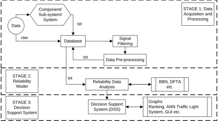
The graphical demonstration of machinery and equipment modelling and analysis data flow is dis-played in Figure 1. It consists of three stages, the data acquisition and processing, the reliability model and

the Decision Support System (DSS). The INCASS MRA is developed in Java Object Oriented Program-ming (OOP) language, whereas the DSS development takes place in R programming language.

Database Signal Filtering

Data Pre-processing Data

Reliability Data Analysis Component/

Sub-system/ System

raw

txt

txt

txt

BBN, DFTA etc.

Decision Support System (DSS)

Graphs

Ranking, ANN Traffic Light System, GUI etc.

STAGE 1: Data Acquisition and

Processing

STAGE 2: Reliability Model

STAGE 3: Decision Support System

Figure 1. Machinery & equipment modelling & analysis data flow.

3.1 Machinery Risk Analysis (MRA) Methodology Firstly, the MRA methodology includes the gath-ering of data in order to process them. Data are cate-gorized among historical, expert and real time moni-toring. Raw data (unprocessed information collected from experts and onboard sensors), are transformed to data input for the MRA methodology. The col-lected data is classified by component, sub-system and main system levels.

All gained information is stored in the database utilizing text (.txt) files. This format file is selected as files are small in size and can be easily transferred from the onboard to the onshore. The following phase involves the real monitoring signal processing. At this phase, signals are filtered and unnecessary infor-mation gathered from the environment of operation is removed. The following critical phase is the transfor-mation of physical sensorial measurements to relia-bility inputs.

In Stage 2 ‘Reliability Model’, the processed reli-ability input data from the database are introduced. The risk and reliability model employs a network ar-rangement similar to the BBNs. This selection allows the probabilistic and mathematical modelling by con-sidering actual functional relations and system/sub-system/component interdependencies.

The third stage of the INCASS model implements Decision Support System (DSS) aspects. The DSS methodology is divided into two sections. The first one is utilized for local (onboard) and short term de-cision making, whereas the second one is used on-shore (global) for longer term predictions and deci-sion features.

The INCASS methodology so far demonstrates the procedures on the data flow level. Hence, it presents the analysis from an input manipulation perspective. In the following figure (Figure 2), the analysis takes place on the specific MRA process and modelling level.

First principles analysis of the parts’ reliability (i.e. wear and tear etc.)

Raw Data

INCASS MRA Model

Results Data preparation &

Pre-processing Data Analysis Methods

Component reliability inputs (i.e. λ, MTBF, PoF etc.)

Figure 2. Machinery Risk Analysis (MRA) process diagram.

As can be seen, INCASS project introduces two main tools the MRA and DSS. On the data flow level, the description incorporates data handling from the data

are employed for the condition and failure diagnostics as well as signal pattern recognition of the received and pre-processed data input. The filtered/processed data is transformed into component reliability inputs such as failure rates (λ), Mean Time Between Failures (MTBF) and Probability of Failure (PoF).

Lastly, the INCASS MRA model aims to predict the future condition of the under investigation ship machinery and equipment. This prognostic feature tends to forecast the failure occurrence (failure modes and events), the time that this failure will take place as well as the components, sub-systems and systems that will be affected.

3.2 Reliability Modelling Tools Review

Various reliability modelling tools are reviewed such as the Fault Tree Analysis (FTA), Event Tree Analy-sis (ETA) and Bayesian Belief Networks (BBNs) in order to select the appropriate for the INCASS MRA modelling requirements. Furthermore in this section, the advantages of time dependent probabilistic relia-bility modelling are demonstrated.

The most known and well applied reliability mod-elling tools include the FTA, ETA, BBN and their dy-namic models of DFTA and DBN respectively. Each of these tools has advantages and limitations, which allow different modelling flexibility levels and selec-tion of failure case scenarios. Furthermore, dynamic modelling introduces reliability time dependencies by simulating failure rates or PoF in various discrete time slices.

According to Bedford and Cooke (2001), FTA is a modelling tool employed as part of quantitative anal-ysis of systems. It is basic tool in system analanal-ysis, which allows pictorial representation of statement in Boolean logic (i.e. 0 or 1, yes or no etc.). FTA devel-ops a deterministic description of the occurrence of an event (the top event). Fault trees analyze the com-ponent failure which contributes to system failure. Furthermore, FTA most usually employs the Boolean operations and, or and not (Kumamoto and Henley, 1996).

A typical fault tree arrangement is developed from top to bottom, while calculations of the failure case scenarios are generated from the bottom basic events determining the failure of the top event. The sequence of events is built by logic gates (Lazakis et al., 2010). In the case of Dynamic FTA (DFTA), the Probability of Working (PoW) is updated continuously by chang-ing condition and value through time. In other words, time dependencies of the operational conditions are introduced. Hence, the dynamic risk modelling of FTA employs the dynamic logic gates.

In contrast with FTA, ETA utilizes ‘forward logic’. Hence, it begins with an initiating event (i.e. non-standard functional case) and propagate this event through the system by considering all possible

routes/options that can affect the behavior of the sys-tem (Bedford and Cooke, 2001).

The third and most critical under consideration quantitative risk tool is the BBN. The main advantage of this tool is the flexible arrangement of the involved systems/sub-systems/components and failure modes (Taheri et al., 2014).

Network arrangement allows the innovative notion of interconnectivities between systems/sub-sys-tems/components. In other words, networks present the interdependency of units. On the other hand, BBN introduces the functions of cost and decision by em-ploying utility nodes (Dikis et al., 2014).

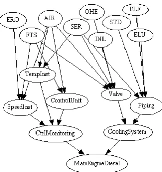
An example of a BBN model is presented in Figure 3 for a diesel Main Engine (M/E). This model demon-strates an extract of the reliability tool developed for the INCASS MRA. The system/sub-systems/compo-nents and the Failure Modes (FMs) are presented in ‘nodes’ while they demonstrate the input gates that the reliability data will be inserted. The arrows pre-sent the connections between the FMs and the com-ponents/sub-systems and main system.

Figure 3. Bayesian Belief Network arrangement.

The BBNs can be defined as probabilistic graphical models involving conditional dependencies arranged into Directed Acyclic Graphs (DAG) and the func-tional relations are mathematically expressed as pre-sented in Equation 1.

𝑃(𝐴|𝐵) =𝑃(𝐵|𝐴) ∗ 𝑃(𝐴)

𝑃(𝐵) (1)

Where P(A) and P(B) are the probabilities of events A and B, while A given B and B given A are condi-tional probabilities. Equation 1 is known as Bayes’ Theorem.

3.3 MRA Reliability Modelling

In the case of dynamic modelling, the time dependen-cies and state division of the reliability input are de-veloped in parallel with the network model. The MRA application employs the mathematical tool of Markov Chains (MC) (Fort et al., 2015). MC is math-ematical system that undergoes transitions from one state to another on a state space. Furthermore, MC is selected as it is flexible to set up by allowing different levels of state sequence complexity.

In order to understand the dynamic probabilistic modelling, a schematic diagram is presented in Figure 4. The presented sub-system sample includes in total three states within the timeline. Firstly, historical pro-cessed data from the previous time slice are provided shown as t-1. The current state (t) is calculated, whereas the predictive state is shown as future state t+1. As it can be seen in Figure 4, each time slice (t-1, t, t+1) is based on the previous state. This single state transition from past to present and then to fore-casted future is known as Markov Chain (MC). The generic probabilistic expression is shown in Equation 2. On the other hand, Equation 3 presents the PoW per expressed component/sub-system in the future t+1 time slice. Where, P(wt+1) denotes the PoW in fu-ture state (t+1) by taking into account previous work-ing and failwork-ing states P(wt) and P(ft) respectively.

Figure 4. Dynamic probabilistic network arrangement.

𝑃𝑋(𝑛−1),𝑋(𝑛)= 𝑃{𝑋𝑡𝑛 = 𝑋𝑛|𝑋𝑡𝑛−1 = 𝑋𝑛−1} (2)

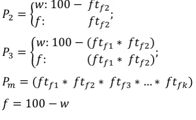
𝑃(𝑤_𝑡+1) = 𝑃(𝑤|𝑤_𝑡)𝑃(𝑤_𝑡) + 𝑃(𝑤|𝑓_𝑡)𝑃(𝑓_𝑡) (3) While, each component of a sub-system is linked with a certain number of failure modes that varies between components, a generic form expressing the failure case scenarios is presented in Equation 7. In this ex-pression, P denotes the Probability of Survival (PoS) for different failure scenarios, where w shows the PoW state while f shows the PoF. The relation of w and f is shown in in Equation 8. Whereas, ftfn indi-cates the failure mode (i.e. noise, vibration, overheat-ing etc.).

Specifically, P1 denotes the PoW and PoF states while one failure mode takes place (ftf1) (Equation 4). Ac-cordingly, P2 denotes the PoW state for a different failure mode (ftf2) (Equation 5). Whereas, P3 repre-sents the PoW and PoF states while ftf1 and ftf2 take place at the same time (Equation 6).

𝑃₁ = {_{𝑓: 𝑓𝑡}𝑤: 100 − 𝑓𝑡𝑓1

𝑓1; (4)

𝑃₂ = {_{𝑓: 𝑓𝑡}𝑤: 100 − 𝑓𝑡𝑓2

𝑓2; (5)

𝑃₃ = {_{𝑓: (𝑓𝑡}𝑤: 100 − (𝑓𝑡𝑓1∗ 𝑓𝑡𝑓2)

𝑓1∗ 𝑓𝑡𝑓2); (6)

𝑃_𝑚 = (𝑓𝑡_𝑓1∗ 𝑓𝑡_𝑓2∗ 𝑓𝑡_𝑓3∗ … ∗ 𝑓𝑡_𝑓𝑘) (7)

𝑓 = 100 − 𝑤 (8)

4 MRA APPRLICATION

In this section, two MRA case studies are presented by involving different ship machinery and equipment systems such as the Turbocharger (T/C) and cargo pump. The case studies examine the working state re-liability performance on system, sub-system and component levels by involving various failure modes as well as failure case scenarios. Furthermore, the case studies utilize processed data in the form of fail-ure rates (λ) per component. The input data is sourced from OREDA database and the entire programmed al-gorithm is developed in Java Object Oriented Pro-gramming (OOP) language.

4.1 Case Study 1

This case study involves the reliability performance of the Turbocharger (T/C). This system is divided in four sub-systems such as the expander and re-com-pressor turbine, control and monitoring, lubrication and the shaft and seal. Each of these sub-systems con-sists of multiple, related in function, components. An extract of these sub-systems is shown in Figure 5, where the control and monitoring and the shaft and seal sub-systems are demonstrated as well as the rel-evant components and involved failure modes.

Figure 5. Turbocharger MRA network case study.

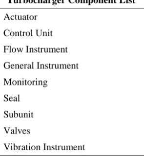
and the shaft and seal). Table 1 lists the turbocharger components.

Table 1. Turbocharger component list.

Turbocharger Component List

Actuator Control Unit Flow Instrument General Instrument Monitoring Seal Subunit Valves

Vibration Instrument

Additionally, Table 2 presents the failure mode selec-tion for the MRA Turbocharger case study.

Table 2. Failure mode selection for MRA T/C case study.

Failure Mode Abbreviation Meaning

AIR - Abnormal Instrument Reading ERO - Erratic Output

ELP - External Leakage – Process Medium (i.e. oil, gas, con-densate, water)

ELU - External Leakage – Utility Medium (i.e. lubricant, cooling water)

FTS - Fail To Start on demand SER - Minor in-service problems UST - Spurious Stop

VIB - Vibration

Hence, in the T/C study a total of four sub-systems, sixteen components and eight failure modes are in-volved.

4.2 Case Study 2

The second case study involves a critical system of tanker ships; that is the cargo pump system. Tanker ships are equipped with multiple cargo pumps (2-3 pumps). For the purpose of this paper, the case study will be presented for one of them while the modelling is similar for all cargo pumps. For this system, eleven failure modes and five sub-systems such as the con-troller, shell, cooling, couplers, and mechanical power are considered. Moreover, these sub-systems include sixteen components. The degradation predic-tions take place on system, sub-system and compo-nent level. Figure 6 demonstrates an extract of the cargo pump network. It presents the controller and mechanical power sub-systems as well as their in-volved components and failure modes.

Figure 6. Cargo pump MRA network case study.

Table 3 demonstrates the case study cargo pump com-ponent list.

Table 3. Cargo pump component list.

Cargo Pump Component List

Actuator Bearing Cabling Control Unit Impeller Monitoring Radial Bearing Shaft

Thrust Bearing

Lastly, Table 4 lists the cargo pump failure modes as involved in this case study.

Table 4. Failure mode selection for MRA Cargo pump case study.

Failure Mode Abbreviation Meaning

AIR - Abnormal Instrument Reading BRD - Breakdown

ELU - External Leakage – Utility Medium (i.e. lubricant, cooling water)

ERO - Erratic Output

FTS - Fail To Start on demand NOI - Noise

OHE - Overheating

5 RESULTS

This section presents the results of the two case stud-ies. The outcomes are demonstrated on component, sub-system and system level while different failure modes are considered including the combination of various failure case scenarios. At present, the time slices for both case studies are considered as unitless values. This is due to the fact that INCASS MRA case studies currently employ processed data from exter-nal sources (e.g. OREDA database) in which the time steps are unknown. Because the processed data is pro-vided in observed failure rates per 106 _operational hours, the time intervals of the predicted states cannot be specified, hence the results are demonstrated as unitless. Whereas, the final MRA application per-forms by employing real time monitored data that their record interval will be known. Hence, when these real time monitored data are applied within the MRA, the time slices will gain actual unit in time as required (i.e. per second, minute, week, month etc.). 5.1 Case Study 1 Results

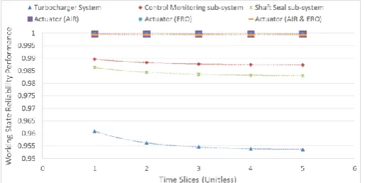
An extract of the Turbocharger (T/C) case study is demonstrated in Figure 7. The results provide the working state reliability performance for the main system (T/C), two sub-systems (i.e. control monitor-ing and shaft and seal) and the actuator component. The actuator’s degradation is examined through three failure case scenarios. Firstly, the actuator reliability performance is shown in case AIR failure mode takes place. Furthermore, the results of the second and third failure case scenarios are presented including the ac-tuator ERO failure mode as well as the combination of the AIR and ERO failure modes.

Figure 7. T/C reliability performance at system/sub-sys-tem/component levels.

The case study performs reliability assessment on system, sub-system and component levels. The mini-mum reliability performance was recorded for the seal component at 83.8%, while the maximum relia-bility at 99.99% for various components. The results show acceptable reliability levels. However, the fol-lowing research phase involves the specification of warning levels and identification of the lowest ac-ceptable reliability outcomes.

5.2 Case Study 2 Results

Similarly, an extract of the cargo pump case study is presented in Figure 8. The outcomes demonstrate the working state reliability performance for the main system, sub-systems (i.e. controller and mechanical power) and the bearing component. The bearing’s re-liability performance is assessed through three failure case scenarios. Firstly, the probability of FTS taking place is examined, followed by the case of NOI oc-currence. Lastly, the probability of both failure modes happening is presented.

Figure 8. Cargo pump reliability performance at system/sub-sys-tem/component levels.

6 DISCUSSION

The developed INCASS MRA methodology is ap-plied on two case studies. The Turbocharger (T/C) and the cargo pump system are involved. Each system is divided into sub-systems and components. Moreo-ver, the components are linked with failure modes that can be affected and lead to failure. The results of these case studies develop various failure case scenar-ios by involving all components, sub-systems, failure modes.

The presented outcomes show the working state reliability performance in five predicted time slices. The prediction of the condition takes place on a sys-tem, sub-system and component level by involving a number of failure case scenarios. The time intervals are considered as unitless. The reason of this assump-tion is that currently INCASS MRA case studies em-ploy processed data from external sources for which the time steps are unknown. However, because MRA will employ real time monitored data, the time slices will gain actual unit in time as required (i.e. per sec-ond, minute, week, month etc.).

sub-systems. Moreover, the performance of the bear-ing is presented includbear-ing the FTS, NOI and both fail-ure modes occurring at the same time.

In conclusion, the MRA’s results are validated in different stages. Firstly, two commercial software are used such as GeNIe 2.0 and Hugin. Moreover, experts such as Classification Societies, ship owners/ opera-tors/ managers and service providers confirmed the acceptable levels of the performed results. In addi-tion, experts verified the system network arrangement and the failure mode selection.

7 CONCLUSIONS

This paper aims to present the development of IN-CASS (Inspection Capabilities for Enhanced Ship Safety) Machinery Risk Analysis (MRA) methodol-ogy. First of all, the paper reviews the most applicable CM tools aiming to select the required for the MRA. The suggested MRA methodology is presented on data and process levels. Lastly, two case studies are demonstrated for the T/C and the cargo pump by pre-senting the dynamic (time dependent) working state reliability performance at system, sub-system and component level by involving various failure modes and failure case scenarios.

Concluding, future research steps include the im-plementation of warning and alarm/risk threshold to be set, in order to gain practical information of the re-liability predictions. Moreover, different MC orders will be tested on MRA aiming to gain longer accurate predictions through time.

8 ACKNOWLEDGEMENTS

INCASS project has received research funding from the European Union’s Seventh Framework Pro-gramme under grant agreement no 605200. This pub-lication reflects only the author’s views and European Union is not liable for any use that may be made of the information contained herein.

REFERENCES

AL-NAJJAR, B. (1996) Total quality maintenance: An approach for continuous reduction in costs of quality products. Journal of Quality in Maintenance Engineering, 2, 4-20.

BAGAVATHIAPPAN, S., LAHIRI, B. B., SARAVANAN, T., PHILIP, J. & JAYAKUMAR, T. (2013) Infrared thermography for condition monitoring – A

review. Infrared Physics & Technology, 60,

35-55.

BEDFORD, T. & COOKE, R. (2001) Probabilistic Risk Analysis: Foundations and Methods, Cambridge University Press.

DHILLON, B. S. & LIU, Y. (2006) Human error in maintenance: a review. Journal of Quality in Maintenance Engineering, 12, 21-36.

DIKIS, K., LAZAKIS, I. & TURAN, O. (2014) Probabilistic Risk Assessment of Condition Monitoring of Marine Diesel Engines. International Conference on Maritime Technology. Glasgow, UK, University of Strathclyde, Glasgow.

IACS (2004) Procedural Requirements for Thickness Measurements. United Kingdom.

INCASS (2014) Deliverable D4.1 Machinery and equipment requirement specification. INCASS - Inspection Capabilities for Enhanced Ship Safety. EC FP7 Project.

JIANG, R. & YAN, X. (2008) Condition Monitoring of Diesel Engines. Complex System Maintenance Handbook. Springer London. KIM, J. & LEE, M. (2009) Real-time diagnostic

system using acoustic emission for a cylinder liner in a large two-stroke diesel engine. International Journal of Precision Engineering and Manufacturing, 10, 51-58. KUMAMOTO, H. & HENLEY, E. J. (1996)

Probabilistic risk assessment and management for engineers and scientists, IEEE Press.

LAZAKIS, I., TURAN, O. & AKSU, S. (2010) Increasing ship operational reliability through the implementation of a holistic maintenance management strategy. Ships and Offshore Structures, 5, 337-357.

MADU, C. N. (2000) Competing through maintenance strategies. International Journal of Quality & Reliability Management, 17,

937-949.

MECHEFSKE, C. K. (2005) Machine Condition Monitoring and Fault Diagnosis, Boca Raton, Florida, USA, CRC Press, Taylor & Francis Group.

MOBLEY, K., HIGGINS, L. & WIKOFF, D. (2008) Maintenance Engineering Handbook, Mcgraw-hill.

MONITION, V. A. (2014) Monition Vibration Analysis for Everyone. Nottinghamshire, United Kingdom.

SHREVE, D. H. (2003) Integrated Condition Monitoring Technologies. Chester, UK, IRD Balancing LLC.