Propagating and Mitigating Uncertainty in the Design of
Complex Multidisciplinary Systems
Thesis by Daniel P. Thunnissen
In Partial Fulfillment of the Requirements for the Degree of
Doctor of Philosophy
California Institute of Technology Pasadena, California
2005
Acknowledgments
Frederick Douglass once said “If there is no struggle, there is no progress.” I think this statement describes my PhD experience here at Caltech well. In ways the past four and half years have been more challenging than I expected yet also more rewarding than I anticipated. This journey would not have been possible without the financial and emotional support of my family and the guidance of my advisors present and past: Professors Fred Culick (Caltech), Victoria Coverstone (University of Illinois at Urbana–Champaign), and Alec Gallimore (University of Michigan). Their support of my education transformed a possibility of a PhD from a dream, to a hope, and now to a reality.
I want to thank my Ph. D. advising committee: Professors Erik Antonsson, Jim Beck, and John Ledyard. All three provided invaluable insight and knowledge, especially Professor Beck who assisted with the subset simulation work. Along with Professor Culick, my advising committee gave me the liberty to pursue research ideas and shielded me from many bureaucratic and financial issues a PhD requires. I also thank Dr. Joel Sercel who provided the initial impetus and research ideas that this thesis became and Melinda Kirk for administrative support.
This thesis builds upon work by a variety of researchers including Professor Ivan Au (Nanyang Technological University, Singapore), Dr. Dan DeLaurentis (Georgia Tech), Dr. Seth Guikema (Cornell University), Dr. William Oberkampf (Sandia National Laboratories), and Dr. Myles Walton (CIBC World Markets). Their work helped motivate directions for my research and many of their PhD themes and goals are mirrored in this thesis. Myles (PhD MIT 2002) and Seth (PhD Stanford 2003), along with Cyrus Jilla (PhD MIT 2002), deserve a special
I would like to thank SSPARC and Northrop Grumman Space & Technology (Redondo Beach, CA) for their financial support of my education here at Caltech. I gratefully acknowledge the Jet Propulsion Laboratory for allowing me to use the Mars Exploration Rover (MER) project as a case study for this research. I would especially like to thank MER team members Mark Adler, Barry Goldstein, Genvieve Lopez, Barry Nakazono, Ralph Roncoli, Ed Swenka, Glenn Tsuyuki, and K. Charles Wang who provided assistance and answers above and beyond their responsibilities. It is to the members of the MER project team that I dedicate this thesis.
Abstract
As humanity has developed increasingly ingenious and complicated systems, it has not been able to accurately predict the performance, development time, reliability, or cost of such systems. This inability to accurately predict parameters of interest in the design of complex
multidisciplinary systems such as automobiles, aircraft, or spacecraft is due in great part to uncertainty. Uncertainty in complex multidisciplinary system design is currently mitigated through the use of heuristic margins. The use of these heuristic margins can result in a system being overdesigned during development or failing during operation.
This thesis proposes a formal method to propagate and mitigate uncertainty in the design of complex multidisciplinary systems. Specifically, applying the proposed method produces a rigorous foundation for determining design margins. The method comprises five distinct steps: identifying tradable parameters; generating analysis models; classifying and addressing
uncertainties; quantifying interaction uncertainty; and determining margins, analyzing the design, and trading parameters. The five steps of the proposed method are defined in detail. Margins are now a function of risk tolerance and are measured relative to mean expected system performance, not variations in design parameters measured relative to heuristic values.
As an example, the proposed method is applied to the preliminary design of a spacecraft attitude determination and control system. In particular, the design of the attitude control system on the Mars Exploration Rover spacecraft cruise stage is used. Use of the proposed method for the example presented yields significant differences between the calculated design margins and the values assumed by the Mars Exploration Rover project.
Table of Contents
Chapter 1 Introduction ... 1
1.1 Motivation and Background... 1
1.2 Space Systems... 6
1.3 Problem Statement ... 19
1.4 Key Contributions and Organization of Thesis... 21
Chapter 2 Uncertainty Classifications and Types ... 23
2.1 Uncertainty and Its Classification in Other Fields ... 24
2.2 Uncertainty Types ... 35
2.3 Summary ... 41
Chapter 3 Method Development and Overview... 43
3.1 Previous Work... 43
3.2 Method Steps and Key Concepts ... 48
3.3 Qualitative Benefits of Method... 51
3.4 Quantitative Results in Applying Method... 55
3.5 Summary ... 56
Chapter 4 Identifying Tradable Parameters ... 57
4.1 Tradable Parameters... 57
4.2 Common Tradable Parameters... 60
4.3 Summary ... 63
Chapter 5 Generating Analysis Models ... 65
5.1 Model Formulation... 65
5.2 Model Uncertainty ... 68
5.3 Phenomenological Uncertainty ... 77
5.4 Summary ... 82
Chapter 6 Classifying and Addressing Uncertainties... 83
6.1 Ambiguity and Aleatory Uncertainty... 83
6.2 Behavioral Uncertainty ... 86
6.3 Importance of Uncertainty ... 93
6.4 Summary ... 95
Chapter 7 Interaction Uncertainty and Simulation... 97
7.1 Existing Simulation Techniques... 97
7.3 Simulation Techniques Ruled Out ... 108
7.4 Simulation Technique Repetitions Required... 111
7.5 Summary ... 112
Chapter 8 Determining Margins, Analyzing the Design, and Trading Parameters... 115
8.1 Determining Margins ... 115
8.2 Analyzing the Results ... 116
8.3 Trading Parameters ... 118
8.4 Summary ... 121
Chapter 9 Application Example – Attitude Determination and Control System ... 123
9.1 Mars Exploration Rover (MER) Project ... 123
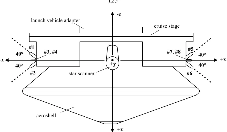
9.2 Attitude Determination and Control System Overview ... 124
9.3 Uncertainties Involved ... 125
9.4 Tradable Parameters... 126
9.5 Models and Model Uncertainty... 127
9.6 Uncertainty Quantification... 136
9.7 Interaction Uncertainty... 138
9.8 Margins and Analysis... 150
9.9 Summary ... 152
Chapter 10 Concluding Remarks ... 153
10.1 Concerns About the Proposed Method ... 154
10.2 Potential Impact of the Proposed Method... 159
10.3 Future Directions ... 162
10.4 Final Thoughts ... 164
Appendix A Mathematical Foundations ... 167
A.1 Probability and Statistics... 167
A.2 Bayesian Techniques... 176
Appendix B Application Examples ... 183
B.1 Propulsion ... 183
B.2 Thermal Control ... 200
B.3 Mission Design... 212
Appendix C Implementation... 215
C.1 General Implementation... 215
List of Figures
Fig. 1.1 The design process; adapted from Pahl and Beitz (1996). ... 3
Fig. 1.2 Decisions made early in design have a significant impact [Symon & Dangerfield, 1980; Thuesen & Fabrycky, 2001]... 5
Fig. 1.3 MER mass history. ... 15
Fig. 2.1 Uncertainty classifications in economics... 26
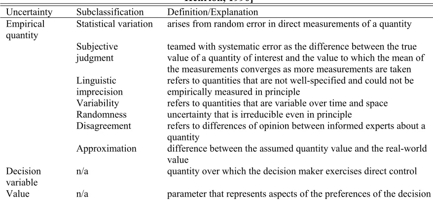
Fig. 2.2 Uncertainty classification in policy & risk analysis [Morgan & Henrion, 1990]. ... 26
Fig. 2.3 Uncertainty classification in systems engineering [Klir & Folger, 1988; INCOSE Systems Engineering Handbook, 2000]. ... 28
Fig. 2.4 Uncertainty classification in civil engineering [Ayyub & Chao, 1998]. ... 29
Fig. 2.5 Uncertainty classification in structural engineering [Melchers, 1999]... 30
Fig. 2.6 Uncertainty classification in computational modeling & simulation [Oberkampf et al., 1999]. ... 31
Fig. 2.7 Uncertainty classification in computational modeling & simulation (mathematical model) [Oberkampf, Helton, & Sentz, 2001]... 32
Fig. 2.8 Alternate uncertainty classification in computational modeling & simulation [Du & Chen, 2000]. ... 32
Fig. 2.9 Uncertainty classification in mechanical engineering [Otto & Antonsson, 1993]. ... 33
Fig. 2.10 Uncertainty classification in aerospace vehicle synthesis and design [DeLaurentis & Mavris, 2000]. ... 33
Fig. 2.11 Uncertainty classification in aircraft systems design [DeLaurentis, 1998]. ... 34
Fig. 2.12 Uncertainty classification in space architectures [Walton, 2002]... 35
Fig. 2.13 Uncertainty classification for the design of complex systems... 36
Fig. 3.1 Example utility functions... 44
Fig. 4.1 Simple schedule [Thunnissen, 2004a]. ... 62
Fig. 4.2 Possible cost and funding profile for a project. ... 63
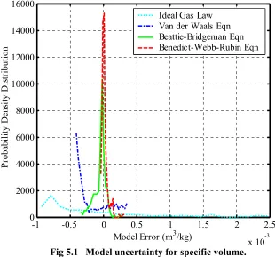
Fig 5.1 Model uncertainty for specific volume... 71
Fig. 5.2 Example relation between verbal expression and assigned likelihood; adapted from Kent (1964). ... 74
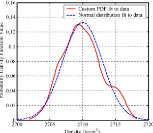
Fig. 6.1 6061-T6 aluminum density uncertainty representation. ... 84
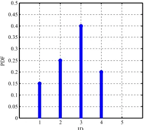
Fig. 6.2 PDF of component choices for tubing. ... 87
Fig. 9.1 MER spacecraft during cruise to Mars. ... 124
Fig. 9.2 MER engine cluster configuration; adapted from D’Amario (2002)... 125
Fig. 9.3 Thrust and exhaust velocity as a function of inlet pressure... 130
Fig. 9.4 Propellant mass PDFs for MCS, LHS, and MMVM. ... 139
Fig. 9.5 Propellant mass CDFs (simulation level 1). ... 140
Fig. 9.6 Propellant mass CDFs (simulation level 2). ... 140
Fig. 9.7 Propellant mass CDFs (simulation level 3). ... 141
Fig. 9.8 Propellant mass CDFs (simulation level 4). ... 141
Fig. 9.9 Schedule duration PDFs for MCS, LHS, and MMVM... 143
Fig. 9.10 Schedule duration CDFs (simulation level 1)... 144
Fig. 9.11 Schedule duration CDFs (simulation level 2)... 144
Fig. 9.12 Schedule duration CDFs (simulation level 3)... 145
Fig. 9.13 Schedule duration CDFs (simulation level 4)... 145
Fig. 9.14 Total cost PDFs for MCS, LHS, and MMVM... 147
Fig. 9.15 Total cost CDFs (simulation level 1)... 148
Fig. 9.16 Total cost CDFs (simulation level 2)... 148
Fig. 9.17 Total cost CDFs (simulation level 3)... 149
Fig. 9.18 Total cost CDFs (simulation level 4)... 149
Fig. A.1 Two distributions with identical means and standard deviations. ... 168
Fig. A.2 PDFs of four continuous distributions (gamma, normal, lognormal, & uniform). ... 170
Fig. A.3 PDFs of two discrete distributions (binomial & uniform). ... 171
Fig. A.4 PDF (left) and CDF (right) for a discrete and continuous triangle distribution with parameters 20, -5, and +5... 172
Fig. A.5 Probability of injected capability greater than spacecraft wet mass. ... 174
Fig. A.6 Example of stochastic dominance... 176
Fig. A.7 Four possible prior distributions in launch vehicle example. ... 178
Fig. A.8 The effect of observations in launch vehicle example... 179
Fig. A.9 Posterior based on first 15 (left) and 30 (right) Delta II launches. ... 179
Fig. A.10 Posterior based on first 45 (left) and 60 (right) Delta II launches. ... 180
Fig. A.11 Posterior based on first 75 (left) and 90 (right) Delta II launches. ... 180
Fig. A.12 Posterior based on first 105 (left) and all 115 (right) Delta II launches. ... 180
Fig. B.1 Propellant mass PDFs for MCS and MMVM... 186
Fig. B.2 Propellant mass CDFs (simulation level 1)... 186
Fig. B.4 Propellant mass CDFs (simulation level 3)... 187
Fig. B.5 Propellant mass CDFs (simulation level 4)... 188
Fig. B.6 Dry mass PDFs for MCS and MMVM. ... 189
Fig. B.7 Dry mass CDFs (simulation level 1)... 190
Fig. B.8 Dry mass CDFs (simulation level 2)... 190
Fig. B.9 Dry mass CDFs (simulation level 3)... 191
Fig. B.10 Dry mass CDFs (simulation level 4)... 191
Fig. B.11 Schedule duration PDFs for MCS and MMVM. ... 193
Fig. B.12 Schedule duration CDFs (simulation level 1). ... 193
Fig. B.13 Schedule duration CDFs (simulation level 2). ... 194
Fig. B.14 Schedule duration CDFs (simulation level 3). ... 194
Fig. B.15 Schedule duration CDFs (simulation level 4). ... 195
Fig. B.16 Total cost PDFs for MCS and MMVM. ... 196
Fig. B.17 Total cost CDFs (simulation level 1). ... 197
Fig. B.18 Total cost CDFs (simulation level 2). ... 197
Fig. B.19 Total cost CDFs (simulation level 3). ... 198
Fig. B.20 Total cost CDFs (simulation level 4). ... 198
Fig. B.21 Maximum component temperature PDFs for MCS and DS. ... 202
Fig. B.22 Maximum component temperature CDFs for MCS and DS... 203
Fig. B.23 Total thermal mass PDFs for MCS and DS. ... 204
Fig. B.24 Total thermal mass CDFs for MCS and DS... 205
Fig. B.25 Power required PDFs for MCS and DS. ... 206
Fig. B.26 Power required CDFs for MCS and DS... 206
Fig. B.27 Schedule duration PDFs for MCS and DS... 207
Fig. B.28 Schedule duration CDFs for MCS and DS. ... 208
Fig. B.29 Total cost PDFs for MCS and DS... 209
Fig. B.30 Total cost CDFs for MCS and DS. ... 209
List of Tables
Table 1.1 Typical spacecraft subsystems... 6
Table 1.2 Recommended hardware mass and power margins [Yarnell, 2003]... 13
Table 1.3 Recommended cost margins [Yarnell, 2003]... 13
Table 1.4 MER flight system margins [Welch, 2001] ... 14
Table 1.5 Design margins for several recent NASA projects ... 16
Table 2.1 Quantity type uncertainty definitions in policy & risk analysis [Morgan & Henrion, 1990] ... 26
Table 2.2 Uncertainty definitions in structural engineering [Melchers, 1999] ... 30
Table 2.3 Incomplete information definitions in computational modeling & simulation... 31
Table 2.4 Uncertainty definitions in computational modeling & simulation (mathematical model) [Oberkampf, Helton, & Sentz, 2001]... 32
Table 2.5 Uncertainty definitions in space architectures [Walton, 2002]... 35
Table 5.1 Examples of modeling tools used in space systems design ... 67
Table 6.1 Possible measured density data of 6061-T6 aluminum ... 84
Table 6.2 Possible component choices for tubing... 86
Table 6.3 Consequence vs. likelihood table; adapted from Conrow (2000)... 95
Table 7.1 Proposal PDFs for different uncertain input variables... 106
Table 9.1 ADCS examples of different uncertainty types ... 125
Table 9.2 Model uncertainties assumed... 135
Table 9.3 General input variables ... 136
Table 9.4 Mission sequence uncertainties... 137
Table 9.5 Deterministic propellant mass results ... 138
Table 9.6 SS results by level for propellant mass ... 142
Table 9.7 Propellant mass calculated by each simulation technique ... 143
Table 9.8 SS results by level for schedule duration... 146
Table 9.9 Schedule duration calculated by each simulation technique... 146
Table 9.10 SS results by level for total cost... 150
Table 9.11 Total cost calculated by each simulation technique... 150
Table 9.12 Calculated (99th percentile) ADCS margin values... 151
Table 9.13 Comparison of assumed and calculated (99th percentile) tradable parameter allocations with actual values... 151
Table A.2 Delta II posterior standard deviations for all four prior distributions ... 181
Table B.1 Model uncertainties assumed ... 183
Table B.2 Updated input variable uncertainties from Thunnissen and Nakazono (2003) ... 184
Table B.3 Deterministic results for thermal control analysis... 184
Table B.4 SS results by level for propellant mass ... 188
Table B.5 Propellant mass calculated by each simulation technique... 189
Table B.6 SS results by level for dry mass ... 192
Table B.7 Dry mass calculated by each simulation technique... 192
Table B.8 SS results by level for schedule duration ... 195
Table B.9 Schedule duration calculated by each simulation technique ... 196
Table B.10 SS results by level for total cost ... 199
Table B.11 Total cost calculated by each simulation technique ... 199
Table B.12 Calculated (99th percentile) margin values for propulsion tradable parameters... 199
Table B.13 Comparison of assumed and calculated (99th percentile) propulsion tradable parameter allocations with actual values... 200
Table B.14 Model uncertainties assumed ... 201
Table B.15 Deterministic results for thermal control analysis... 201
Table B.16 Maximum component temperature calculated by MCS and DS ... 203
Table B.17 Total thermal mass calculated by MCS and DS... 205
Table B.18 Power required calculated by MCS and DS... 207
Table B.19 Schedule duration calculated by MCS and DS ... 208
Table B.20 Total cost calculated by MCS and DS ... 210
Table B.21 Calculated (99th percentile) margin values for maximum component temperatures ... 210
Table B.22 Calculated (99th percentile) margin values for mass, power required, schedule duration, and total cost ... 210
Table B.23 Comparison of assumed and calculated (99th percentile) maximum temperature allocations with actual values... 210
Table B.24 Comparison of assumed and calculated (99th percentile) mass, power required, schedule duration, and total cost allocations with actual values ... 211
Glossary and Nomenclature
A glossary is presented to familiarize the reader with some of the terminology that is introduced and subsequently used throughout the course of this thesis. The terms are consistent with the literature, where the literature itself is consistent.
aleatory uncertainty. Inherent variation associated with a physical system or environment under consideration.
ambiguity. Imprecise terms and expressions used in general communication.
approximation errors. Deficiencies in models where the phenomena or processes are relatively well understood.
asymmetric information. Information available to only a subset of a group and not all the parties involved.
Bayesian techniques. Formal mathematical methods that start with an existing belief and update that belief based on new data.
behavioral uncertainty. Uncertainty in how individuals or organizations act.
complex multidisciplinary system. A combination of two or more subsystems (disciplines) that result in a total system. The complexity is due primarily to the number of subsystems and their interactions with each other; individual subsystem complexity is secondary.
component. A functional item that is viewed as a complete and separate entity for purposes of manufacturing, maintenance, or record keeping. Examples in space systems design include a star tracker, thruster, and an electrical heater.
conceptual design. A short study period on the order of weeks or months to turn an idea into a concept and secure additional funding.
contingency. A synonym of margin or reserve. In some fields contingency is used specifically in design.
cumulative distribution function (CDF). A monotonically increasing mathematical expression that gives the probability that an uncertain quantity is less than or equal to a specific value.
decision maker. One or more individuals or organizations responsible for making final decisions in a project. In this thesis, the singular is used although the decision maker may consist of more than one individual or organization (e.g., the board of directors and the chief executive officer in a private corporation).
design uncertainty. A choice among alternatives over which an individual or individuals exercises direct control but has not yet decided upon. An example is the choice an engineer has in selecting a given component among a set of possible components.
deterministic. A state that does not include or involve uncertainty.
epistemic uncertainty. Any lack of knowledge or information in any phase or activity of the modeling process.
errors. The accuracy of a mathematical model to describe an actual physical system of interest.
human errors. Blunders or mistakes by an individual or individuals during design.
interaction uncertainty. Uncertainty arising from unanticipated interaction of many events and/or disciplines, each of which might, in principle, be or should have been foreseeable.
margin. Variations in parameters (or resources) measured relative to best-estimate values.
mean. Expected value of a random variable.
median. A value of a random variable such that there is a 0.5 probability that the actual value of the variable is less than that value: P[X ≤ X0.5] ≡ 0.5.
mode. The value or values of a random variable that have maximal probability density.
model uncertainty. Accuracy of a mathematical model to describe an actual physical system of interest
numerical errors. Errors that arise due to finite precision arithmetic in a numerical model.
percentile. A value in percent such that there is a probability p that the actual value of a random variable, X, will be less than that value: P[X ≤ Xp] ≡ p. Also known as a fractile or quantile when
expressed as a fraction.
phenomenological uncertainty. Uncertainty that cannot be imagined. Also referred to as “unknown unknowns.”
preliminary design. A more rigorous extension of conceptual design where the development of other options; the creation of risk management strategies; and the refining of previously
performed trades, analyses, and cost estimates are performed.
probabilistic. A state that involves uncertainty represented by random variables instead of fixed and (assumed) known deterministic values.
probability density function (PDF). A mathematical expression that provides the probability of an event for each possible outcome.
programming errors. Mistakes or blunders by a programmer during development of a mathematical model.
random variable. An empirical quantity which is uncertain. Specifically, a real valued function defined on a sample space.
requirement uncertainty. Parameters of interest to and determined by the stake holder, independent of the engineer or designer.
sample. A grouped number of observed random variables.
standard deviation. The square root of the variance. The standard deviation (variance) reflects the amount of spread or dispersion in the distribution.
space system. An integrated set of subsystems and components capable of supporting an
operational role in space. Examples in the field of space systems design include an Earth-orbiting satellite, an interplanetary spacecraft, and a space station.
stake holder. One or more individuals or organizations who own a portion or the entirety of a project or is directly impacted by its outcome. In this thesis, the singular is used although the stake holder may consist of more than one individual or organization (e.g., the stake holder for a government mission is both the government and that country’s citizens).
subsystem. An assembly of functionally related components (e.g., attitude control, propulsion, and thermal control). Also referred to as discipline.
tradable parameter. A quantifiable property that provides a performance measure of the complex multidisciplinary system that can be traded during design against one or more other quantifiable properties (e.g., mass, cost, schedule, and risk).
risk. The likelihood of failure.
uncertainty. The difference between an anticipated or predicted value (behavior) and a future actual value (behavior).
variance. The second central moment of a random variable.
volitional uncertainty. Uncertainty about what a subject him/herself will decide.
Acronyms and abbreviations used throughout the course of this thesis are summarized here: ADCS = attitude determination and control system
A/F = analyst/facilitator
BWR = Benedict-Webb-Rubin
CBE = current best estimate
CDF = cumulative distribution function c.o.v. = coefficient of variation
DoD = Department of Defense
DS = descriptive sampling
FP = fault protection
FY2003$M = fiscal year 2003 dollars in millions (M) INCOSE = International Council on Systems Engineering
JPL = Jet Propulsion Laboratory
LHS = Latin hypercube sampling
MCS = Monte Carlo simulation
MCMC = Markov chain Monte Carlo
MER = Mars Exploration Rover
MMVM = modified mean value method
MoM = method of moments
MPF = Mars Pathfinder
MVM = mean value method
NASA = National Aeronautics and Space Administration PDF = probability density function
PDR = preliminary design review
PRA = probabilistic risk analysis
REM = rover electronics module
SDST = small deep space transponder
SS = subset simulation
SSPA = solid state power amplifier
USAF = United States Air Force
WCE = worst case estimate
Symbols used throughout the course of this thesis are defined here (some have multiple definitions; their context should make it clear what the relevant definition is):
A cross-sectional area, m2
A two column array; first column (A1) is the choice (A1∈ integer), second
column (A2) is the probability of that choice being selected (0 ≤ A2 ≤ 1)
a, b van der Waals constants
A0, a, B0, b, C0, c, α, γ Benedict-Webb-Rubin constants
B(n,p) binomial distribution with parameters n (number of trials) and p (constant probability of success for each trial)
Ci boundary value of “failure region” for simulation level i
Cd(A) discrete custom distribution with parameters listed in the array A
c engine exhaust velocity, m/s
c0 speed of light in a vacuum, 299792458 m/s
D data
d distance from the spacecraft to the sun, AU
F thrust, N
Fi failure region i
Fx xth fractal value (Px /100)
f mathematical function or friction factor; flux, W/m2
G vector function that determines the tradable parameters based on the input variables; may be a computationally expensive function
gs solar constant at 1 AU, W/m2
H hypothesis; angular momentum, kg-m2/s
h step size
I impulse, N-s
IF indicator function (IF = 1 if true, IF = 0 if false)
Ijj,k(i) indicator function for the kth Markov chain sample in the jjth Markov
chain at simulation level i
i subset simulation level
J moment of inertia, kg-m2
j input variable number
jj Markov chain number
k1, k2 thrust constants for a given engine
k3, k4 exhaust velocity constants for a given engine
L(µ,σ) lognormal distribution with parameters µ and σ
m number of conditional levels (indexed with i = 1, …, m); mass, kg N total number of Monte Carlo simulation (MCS) samples; total number of
MCS samples for initial run through (i = 1) subset simulation; total number of Markov chain samples across all chains for subsequent simulation levels (i > 1)
N(µ,σj) normal distribution with parameters µ and σj
N/Nc number of samples in each Markov chain (Markov chain samples starting
from a seed; indexed with k = 1, …, N/Nc)
Nc number of Markov chain seeds (Nc = p0·N; indexed with jj = 1, …, Nc)
n number of input variables (indexed with j = 1, …, n); number or quantity
P probability
Pf specified probability of interest at distribution tail (e.g., Pf = 0.01
corresponds to 99th percentile, Pf = 0.001 to 99.9th percentile, etc.)
Pi specified probability of failure at simulation level i; Pi = P(Fi|Fi-1), i = 2,
…, m
Px xth percentile value
Pi* actual probability of failure at simulation level i
p pressure, Pa
pj* proposal probability density function (PDF) for input variable j
p0 conditional probability specified for subset simulation; p0∈ (0,1)
Qj one-dimensional cumulative distribution function (CDF) for input
variable θ(j)
Qj-1 inverse CDF for input variable θ(j)
q spacecraft surface reflectivity
q vector of one-dimensional PDFs
R engine moment arm, m
Rdet deterministic result value
Ri(k) covariance sequence for subset simulation level i at Markov chain
sample number k
ReD Reynolds number based on diameter
r effective engine moment arm, m
rj ratio used in Metropolis-Hastings algorithm for input variable j
s number of Latin hypercube segments and repetitions
T temperature, K
t number of tradable parameters; time, s
U (continuous) uniform random variable on the interval 0 to 1
U(min,max) (continuous) uniform distribution with parameters “min” and “max” Ud(min,max) discrete uniform distribution with (integer) parameters “min” and “max”
X general random variable
x fraction
Y vector of probabilistic tradable parameters y dependent variable or tradable parameter
y vector of tradable parameters, vector of tradable parameter values at a subset simulation level of interest
α rotational control acceleration, rad/s2
β(a,b) beta distribution with parameters a and b Γ(A,B) gamma distribution with parameters A and B
γ pointing control, rad
γi correlation factor at subset simulation level i
∆c(peak,minus,plus) continuous triangle distribution with parameters peak, minus, plus
∆d(peak,minus,plus) discrete triangle distribution with parameters peak, minus, plus
∆Itorque change in impulse torque, N-m-s
∆τ change in torque, N-m
∆φ angle through which engine(s) are fired, rad
∆ω change in spin rate, rad/s
δ engine misalignment angle, rad
δi coefficient of variation (c.o.v.) of Pi*
δi* total c.o.v. up to and including simulation level i
η engine duty cycle
θi sunlight angle of incidence, rad
θk vector of uncertain input variables at Markov chain sample number k
θk(j) (potentially uncertain) input variable j at Markov chain sample number k
θk* vector of input variable candidate states at Markov chain sample number
k
θk*(j) candidate state for input variable j at Markov chain sample number k
κ distance from the center of pressure to the center of mass, m
λ confidence deviation parameter calculated via the inverse of N(0,1); nutation frequency, Hz
µ mean
ν specific volume, m3/kmol
ξj simulated value generated from proposal PDF for input variable j
ρi(k) correlation coefficient at lag k of the stationary sequence {Ijk(i): k = 1, …,
N/Nc}
σi standard deviation of Pi*
σj standard deviation of one-dimensional PDF qj
τ torque, N-m
ψ slew angle, rad
ω spin rate, rad/s
ℑ force, N
ℜ set of all real numbers or universal gas constant, 8314.51 J/kmol-K
~ round down to nearest integer
~ round up to nearest integer
∅ empty set
∪ union
∩ intersection
Subscripts:
act_tot total actual
f final desired
half_rev half a revolution of the spacecraft about the spin axis
i initial
ideal_tot total ideal
inlet at the engine inlet
j input variable uncertainty number
max maximum min_on engine minimum on per pulse
on engine on per pulse
p_slew propellant required for slewing p_spin propellant required for (de)spinning req required
s solar
sd scaled down
xx axis orthogonal to spin axis
zz spin axis
Superscripts:
i engine number
j thrust maneuver number
k pulse maneuver number, tradable parameter number
t true value
Chapter 1
Introduction
This chapter introduces the research presented in this thesis. The chapter begins with motivation and background concerning uncertainty in engineering design and, specifically, in complex multidisciplinary systems. An overview of space systems, the complex
multidisciplinary system consistently referred to as an example throughout this thesis, follows. Methods of space systems design and uncertainty mitigation in space systems design are then presented. The current method of uncertainty mitigation through the use of heuristic design margins is discussed with an entire section dedicated to design margin examples. Particular attention is paid to the impact the current method of determining these margins has had on space systems design, development, and the aerospace industry in general. The mathematical problem statement this thesis addresses is then described. The chapter ends with a summary of the key thesis contributions and an overview of the remainder of the thesis.
1.1 Motivation and Background
Humans have developed as the dominant species on Earth (with respect to altering lives and the environment). Foremost among the reasons for this is the ability of humans to develop, build, and master instruments and tools. Although many species alter their surroundings for habitation, only a handful of other species use tools (e.g., otters use rocks to open clams, apes use sticks for food gathering). Development of increasingly complex tools by humans followed from similar humble beginnings, an activity that continues to this day. One of the reasons tools have become increasingly complex is uncertainty. Tools (systems) have become complex to reduce uncertainty and allow for reliable predictability. An example which illustrates this well is the missile.
A missile is defined as “an object (as a weapon) thrown or projected usually so as to strike something at a distance” [Webster’s Ninth New Collegiate Dictionary, 1990]. The first missiles were simply rocks hurled by early man to kill animals and other humans. As humankind evolved from hunter gathers to city-states around 8000 BC, the missile evolved from a rock being thrown by man to one shot by a sling and, by c400 BC, one propelled by a catapult. This modest
design of complex systems. Today cruise and ballistic missiles are highly complex systems capable of quickly delivering enormous ordinances over thousands of kilometers while requiring little to no human assistance. The transition from flying bombs to missiles included the addition of sensors, actuators, and computers to counter uncertainties in atmospheric conditions, release conditions, and target movement.
As humanity has developed increasingly ingenious and complicated systems to reduce uncertainties and allow for reliable predictability, humanity has not been able to accurately predict other parameters of interest such as the performance, development time, reliability, or cost of such systems. This inability to accurately predict parameters of interest in the design of complex systems is due in great part to uncertainty. Uncertainty has repeatedly been treated as a supplemental piece of information during design. It is often considered after decisions have been made and sometimes ignored completely. This thesis addresses this issue by proposing a formal method to propagate and mitigate uncertainty in the design of complex systems. One of the goals of this proposed method is to make uncertainty a central concept in the design of these systems. This thesis illustrates the intimate relationship and importance uncertainty has to the entire design, development, and decision-making process.
Uncertainty can result in a system being overdesigned during development or failing during operation. Addressing uncertainty can thus reduce the effort in designing (redesigning) complex systems. It is not always possible to remove uncertainties or even obtain the information
necessary to predict them. Hence, the need remains for a repeatable and mathematically rigorous approach for quantifying these uncertainties to assist a decision maker. A decision maker is one or more individuals or organizations responsible for making final decisions in a project. In this thesis, the singular is used although the decision maker may consist of more than one individual or organization. Probabilistic methods are the cornerstone of this mathematical rigor presented in this thesis and offer a viable approach to mange uncertainties that confront the decision maker. Probability theory is well-known to provide a rational and consistent framework for treating uncertainties and plausible reasoning [Cox, 1961; Papoulis, 1965; Jaynes 1983]. In short, the method proposed in this thesis attempts to improve how complex systems are designed, which remains one of the major contemporary engineering research challenges.
1.1.1 Engineering Design
Engineering design is the process by which systems and products are built to satisfy the needs of customers in a safe, efficient, and reliable manner. Design involves the conception of
solutions) and decision (choice among those alternatives). Engineering design distinguishes itself from other fields of design by its use of calculation and analysis. An integral part of this process is using limited resources to manage uncertainties in the development process and to improve the performance of the system, itself an uncertainty during the design process, once it is placed in service. The engineering design process consists of a number of steps to find a good solution to a specific problem. First there is the statement of a need and a specification of the requirements for the system. This is followed by an exploration of possible forms of solutions to the stated
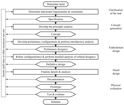
problem, leading to a conceptual design. This conceptual design, a specification of the general type of solution but not of the details of the design itself, then becomes a detailed design, recorded in working drawings and other documentation, through analysis and optimization of its characteristics. The detailed design is then implemented through the process of building, testing, and finally placing in service the resulting system. Throughout this process there is considerable feedback and iteration as shown in Fig. 1.1.
Determine need
Solution
Determine functional requirements & constraints
Specification
Develop the principle solution
Concept
Develop preliminary configurations & perform introductory analysis
Preliminary design(s)
Definitive design
Refine configuration(s) & perform detailed analysis of refined design(s)
Documentation Finalize details & analysis
Prototype
Test & evaluate
Ite
ra
te
unt
il
ti
m
e
or
othe
r re
source
s
run
out
Clarification of the task
Concept generation
Embodiment design
Detail design
[image:27.612.106.536.315.679.2]Physical evaluation
Engineering design research seeks both a strong mathematical foundation and real-world applicability. The two are often connected: a rigorous mathematical foundation helps guarantee the success of an application, while the desire to solve particular problems uncovers needs of the theory. Complex multidisciplinary systems represent the application used in applying the method and theory developed in this thesis.
1.1.2 Complex Multidisciplinary Systems
The major engineering projects of the last half a century and those planned for the current century dwarf those of previous centuries in complexity. The development of the ballistic missile and space programs in the 1960s helped to usher in a new level of complexity in design and building multidisciplinary systems. The fields of systems engineering and project management were formalized during these two programs to assist in their successful development [Sapolsky, 1972]. This formalization is significant in that methods to propagate and mitigate uncertainty in design of complex systems must include and be compatible with these two fields. Missiles, automobiles, aircraft, power plants, submarines, and space systems are all examples of complex multidisciplinary systems. This thesis uses space systems as the archetypal complex
multidisciplinary system in applying formal uncertainty techniques.
Complex multidisciplinary systems require dozens of different specialists to design and significant resources to build. These systems are usually designed by a team of engineers, each with responsibility for a different portion (subsystem) of the design. This design team could be arranged in a number of ways such as traditional (or pyramid) organization, a task-force organization, or a matrix organization. The design team aspect means that there are often asymmetries in information and differing incentives among the team members. Complex multidisciplinary systems are often built by more than one organization since a single
organization rarely has the expertise in all the subsystems required in the design. When multiple organizations are involved, the complexity and informational asymmetries often increase further as interaction among specialists is more difficult.
be significantly different from existing similar designs to allow well-informed design decisions to be made. If the environment is defined as everything outside the complex multidisciplinary system, an increase in complexity of these systems shifts uncertainty from the environment to the subsystems (assemblies, components, etc.) and to the system as a whole. This is a significant system benefit if the subsystems are sufficiently reliable. However, to realize this benefit, explicit models of subsystem uncertainties and the ability to quantify and propagate these uncertainties through the system is critical. Moreover, complex multidisciplinary systems often have a tightly constrained set of resources that further complicates asset allocation and risk management among the various subsystems during design. Hence, the “complex” in complex multidisciplinary systems refers primarily to the complexity in the number and interaction of disciplines (subsystems). The actual “complexity” of an individual subsystem is secondary.
The development of a complex system is characterized by distinct phases: conceptual design; preliminary design; detailed design; manufacturing design; system integration and verification; and operations. Conceptual and preliminary design of complex multidisciplinary systems are characterized by decision making that is separated far from the consequences of such decisions. Hence, although both conceptual and preliminary design entails a relatively low allocation of resources and effort, the decisions made during this stage of the design have significant ramifications. This is shown in Fig. 1.2.
[image:29.612.176.486.419.682.2]
Finally, complex multidisciplinary systems are often designed concurrently, as opposed to sequentially. Concurrent engineering reduces the time of manufacturing and total cost provided the individuals involved in the design process are properly trained and communicate [Burghardt, 1999]. The formal methods to propagate and mitigate uncertainty described in this thesis were developed with concurrent engineering in mind for maximum applicability.
1.2 Space
Systems
A space system is an integrated set of subsystems and components capable of supporting an operational role in space. Space systems range widely from an Earth-orbiting space station to an interplanetary spacecraft. Space systems, specifically spacecraft, are used as examples in applying the method developed in this thesis. Spacecraft differ from other space systems in that they are robotic (i.e., unmanned) systems on the order of tens to a few thousand kilograms. Spacecraft are built by one or more organizations that must have a significant knowledge base in a multitude of disciplines such as structures, thermal control, and propulsion. One or more designer/decision maker represents each of these spacecraft subsystems (disciplines). These subsystems must be integrated together which requires competent systems engineering and management. A summary of typical spacecraft subsystems and their definitions are provided in Table 1.1. More detailed descriptions of spacecraft subsystems are provided in Griffin and French (2004) and Larson and Wertz (1999).
Table 1.1 Typical spacecraft subsystems
Subsystem (Discipline) Definition
Attitude, determination,
and control (ADCS) Orients and stabilizes the spacecraft countering external and internal disturbances that act upon it Command and data
handling (C&DH) Stores and processes commands and data
Management Oversees all other subsystems and disciplines and acts as the liaison
to the mission stake-holders
Mission design Selects launch vehicle(s), analyzes trajectories, and determines
orbital characteristics for all mission phases
Payload Instruments and devices used to achieve the overall
spacecraft/mission goals
Power Generates, conditions, regulates, stores, and distributes power
throughout the spacecraft
Propulsion Provides the changes in velocity needed to translate the center of
mass of a spacecraft and/or to provide a torque to rotate a vehicle about its center of mass
Structures &
mechanisms Supports and protects all other subsystems for all operating modes of the spacecraft and in all of the expected mission phases; deploys components and/or separates from other elements during the mission
Systems engineering Oversees integration and interaction between subsystems
Telecommunications Receives and transmits signals between the spacecraft and ground
Subsystem (Discipline) Definition
Thermal control Maintains all components of a spacecraft within their allowable
temperature limits for all operating modes of the spacecraft and in all of the expected thermal environments
The definitions provided in Table 1.1 illustrate many of the uncertainties a spacecraft encounters in operation that must be accounted for in design. Each of the subsystems listed in Table 1.1 have developed significantly in capability and complexity to handle such uncertainties since the first successful spacecraft (Sputnik) was designed and built in 1957. A recent trend in space systems design is towards spacecraft constellations which are designed to counter
uncertainties in the location where a signal, such as a phone call or missile launch, may be generated. Although built upon relatively established fields of mechanical and aeronautical engineering, aerospace engineering is nascent. Furthermore, much of the aerospace experience is either classified or competition sensitive and not available for analysis. The aerospace industry does not have the benefit of centuries of experience and highly visible and public applications that other engineering fields boast (e.g., civil, mechanical, naval). In short, the statistical base readily available to the aerospace industry is small.
1.2.1 Space Systems Design
Conceptual design; preliminary design; detailed design; manufacturing design; system integration and verification; and operations for space systems are often abbreviated using National Aeronautics and Space Administration (NASA) terminology [INCOSE Systems
Engineering Handbook, 2000]. Conceptual design, referred to as “Pre-phase A,” is a short study period on the order of weeks or months to turn an idea into a concept and secure additional funding. Initial requirements are defined; evaluation criteria are determined; risks are identified; and preliminary trades, analyses, and cost estimates are made. Pre-phase A is typically
years. Manufacturing design and system integration & verification, referred to as “Phase C/D,” is where design is finalized, the spacecraft is developed, integrated, tested, and launched. Phase C/D is on the order of months to years. Finally, operations, referred to as “Phase E,” is the actual period in time of the mission to which the space system was designed. Phase E is on the order of minutes to years depending on the type of mission.
Space systems design durations and costs have changed dramatically in the 50 years they have been built. Early spacecraft were designed and built in months (e.g., early Explorer, Pioneer, and Mariner series spacecraft) and cost on the order of hundreds of millions of current year dollars [Koppas, 1982]. As space system designs became more complex and methods and technologies improved, this time frame became years and billions of current year dollars for many missions (e.g., Space Shuttle; NASA’s Chandra and Cassini; ESA’s Envisat; USAF’s Milstar). Recently, the design time has begun to move back towards the order of months and the cost to hundreds of millions of current year dollars (e.g., NASA’s Mars Pathfinder and Genesis, commercial satellites), due in part to a return to simpler spacecraft designs stressed in NASA’s “faster, better, cheaper” effort of the 1990s. The typical contemporary spacecraft development programs do not typically have the luxury of long times or large budgets for extensive technology development, full system testing, and redesign. Aerospace design has gone from maximizing performance under technology constraints to minimizing cost under performance constraints [Mosher, 1999] and addressing affordability in conceptual design shifts the fundamental question from “can it be built” to “should it be built” [DeLaurentis, 1998]. Space systems today continue to be unique and high unit costs are not amortized in building subsequent models of that design. Upgrading and extending the capability of space systems in orbit is prohibitively expensive and difficult while software upgrades take time on the ground in testing and delay possible revenue-generating operations in space. All these ongoing issues provide opportunities and impetus for research in improving how these systems are designed and built [Thunnissen, 2004a].
1.2.2 Uncertainty Mitigation
addressed as unique, and any calculations of these uncertainties are typically a posteriori and are not embedded in the end model [Walton, 2002]. Moreover, current methods are not amenable to trading resources and parameters of interest such as mass, cost, and time under conditions of uncertainty. The three formal methods currently used to propagate and mitigate uncertainty in space systems design are probabilistic risk analysis (PRA), factors of safety, and design margins. Each is discussed in detail in this section.
1.2.2.1 Probabilistic Risk Analysis
Probabilistic risk analysis (PRA) provides a method to define and measure quantitatively the technical failure risks of engineering systems. PRA was developed in the decades following the Second World War in analyzing the risks of failure of, and the risks imposed on, society by increasingly complex systems. The purpose of a technical PRA is to examine all potential damage states and the frequency of each state as uncertain variables. Early work in PRA focused on simple electronic circuits, leading to the development of fault trees, a tool that has become an integral part of current PRA. The first major program to apply PRA was the Minuteman Missile program. PRA was applied by NASA in estimating catastrophic probabilities for the Apollo program in the late 1960s. This PRA effort yielded such controversial results that it left the aerospace industry reluctant to apply PRA for the following two decades [Seife, 2003].
As the aerospace industry discarded PRA in the 1970s for more traditional methods, PRA developed significantly in the fields of structural engineering, nuclear power plant safety, and chemical processing. The more robust and rigorous PRA that resulted was reintroduced to the field of aerospace engineering following the Challenger accident in 1986 [Feynman, 1986; Paté-Cornell & Fischbeck, 1993]. PRA today uses probabilistic methods, statistical methods, and event trees in addition to fault trees. The quantification of uncertainty with PRA for design is based on a combination of statistical data from past experiences with systems similar to the one being designed, interpretations of test results, and expert opinions. Since appropriate statistical data are often not available, especially in the relatively nascent and competition-sensitive field of aerospace engineering, PRA must frequently rely on expert opinion. PRA has traditionally been used in space systems design to support established design decisions with the goal of justifying a low probability of a technical failure of the system and not a method used for actual design.* However, when applied during design, PRA techniques provide an extremely powerful tool for discovering design errors, inconsistencies, and incompatibilities. Increasingly PRA has been used
*“Sentence first, verdict afterwards, facts sooner or later forgotten.” - Queen of Hearts in Alice in
in conjunction with other methods such as safety factors and design margins in addressing uncertainty. Dillon (1999) and Guikema (2003) describes PRA in detail.
1.2.2.2 Factors of Safety
Safety factors are one of the simplest and most widely used methods of addressing uncertainty. The use of a safety factor is a design philosophy which addresses uncertainty through conservatism in tolerances and operational limits [DeLaurentis, 1998]. This approach, deterministic in nature, seeks to identify the worst possible conditions a product may encounter, and then design the product to perform adequately under such conditions. Factors of safety are often even greater than this union of worst possible conditions to account for “unknown unknowns.”† For example, a factor of safety of 1.5 is often used in pressure vessel design to account for uncertainties in material properties, storage conditions, and operating conditions. Factors of safety in solid mechanics account for uncertainties in static and dynamic loadings. The primary drawback of safety factors is their conservatism. Performance is sacrificed over the range of typical operating conditions for performance guarantees at unlikely or impossible conditions. A design’s true factor of safety can never be known if the ultimate failure mode is unknown. Thus the design that succeeds (i.e., does not fail) can actually provide less reliable information about how or how not to extrapolate from that design than one that fails. It is this observation that has long motivated reflective designers to study failures even more assiduously than successes [Petroski, 1994]. From a pedagogical point of view, the safety factor approach generates no new information about the behavior of the design space which can be exploited in future designs [DeLaurentis, 1998].
1.2.2.3 Design Margins
Conceptual and preliminary design is generally done deterministically, operating as though all quantities of the design are known with complete certainty. Design margins are applied ex post facto to account for the uncertainties in the design because rigorous techniques for uncertainty mitigation and propagation are not available. Design margins are defined as
variations in parameters (or resources) measured relative to best-estimate values. The definition often differs from resource to resource and organization to organization. Design margins are also known as “margins,” “contingencies,” and “reserves.” Margin is often employed when referring to operational resource values, contingencies when referring to design resource values, and reserves when referring specifically to cost. The word margin, not contingency or reserve, is
used in this thesis. Many margins for parameters are expressed as percentages, using worst-case estimate (WCE) and current best estimate (CBE) parameter values:
100 CBE
CBE WCE margin
% current = − ⋅ (1.1)
CBE values can be viewed as deterministic since they represent a best guess point value based on some combination of data, analysis, and technical judgment. However, the basis for many assumptions and the scope of thought that went into estimating CBEs are often not explicitly documented. On their own, CBEs have no degree of confidence associated with them. Furthermore, CBEs are often biased away from the mean values of the uncertainties they
represent. WCE values can be viewed as some combination (perhaps the union) of worst possible conditions. Hence, the “worst” in WCE is subjective.
This definition of design margin appears similar to the definition of factor of safety provided in the previous section. But while factors of safety are typically static during design, design margins vary throughout the development and their allocation range from being capricious to “hope oriented” to overly conservative. Design margins are implemented to allow the various elements of a design team to work in parallel as much as possible. By providing numbers with margin (“holding margin”), a team of a given subsystem or discipline is more insulated from changes occurring in other subsystems or disciplines and can proceed with their design. Design margins are chosen to be robust enough to accommodate uncertainties and enable design changes with minimal system-wide “ripple effects.” Margins maintained vary not only from organization-to-organization, but from individual-to-individual (e.g., project manager-to-chief engineer, chief engineer-to-flight systems engineer) within an organization based on the risk tolerance of that organization or individual or both. The choice in these margins is typically an afterthought and attempts to account for all uncertainties that engineers encounter by lumping these uncertainties into one value with little or no analysis.
For space systems in general, margins not based on a WCE are allocated heuristically, based on historical data, or in a crudely quantitative manner, based on such concepts as design maturity and mission environment. Heuristic is defined as “involving or serving as an aid to learning, discovery, or problem-solving by experimental and especially trial-and-error methods”
[Webster’s Ninth New Collegiate Dictionary, 1990]. For space systems design, the “experimental and especially trail-and-error methods” correspond to previous historical experience by an organization or set of organizations. Heuristics suffer from cognitive biases including
about the item (or variable or quantity) with the stereotypical member of the category.
Availability occurs when judgment about the characteristics of an item is based on the ease with which similar items from memory are recalled. Finally, anchoring and adjusting refers to the notion that in making estimates of an item an initial “anchor” is chosen. That anchor is
subsequently adjusted based on knowledge of the specific item. Heuristic-based design margins tend to be simple, easy to apply, but often lead to severe and systematic errors. The following section provides actual examples that illustrate the current heuristic method of applying design margins in space systems design and their impact.
1.2.3 Design Margin Examples and Impact
As the design of a space system progresses, CBEs of resources typically rise using up the margin that is being held. Significant design and management problems can occur when the rise in the CBEs is greater than the margin being held (“blown margins”). Such systems may have to be redesigned which may result in the system being over budget, delivered late, descoped, or cancelled. On the other hand, holding too much margin early in project design may cause the system to be overdesigned, uncompetitive, and/or poorly managed. Determining the correct margin at various stages of the development is critical in determining the likelihood of success in designing a spacecraft. Examples of applying heuristic and/or historical based methods to determine design margins in space systems design are numerous. Unfortunately, obtaining best estimate and margin values for space system that can be referenced is more difficult. Reasons for this include competition sensitivity, insufficient tracking and recording of values, and reluctance on the part of space system designers to document missions in which margin values have exceeded or missions in which too much margin was held. The following section provides examples of the current method of applying margins to NASA, Department of Defense (DoD), and commercial missions. The section concludes with some examples of margin application in other fields. All examples are referenced.
1.2.3.1 NASA Spacecraft
included mission/system design changes, design complexity, amount of inheritance, amount of new technology/concepts, quality/fidelity of early estimates, and funding available [Yarnell, 2003]. Such analyses resulted in the recommended margins (relative to a preliminary mission system review) for hardware mass and power using a maturity-based approach as shown in Table 1.2.
Table 1.2 Recommended hardware mass and power margins [Yarnell, 2003]
Hardware Recommended Margin (%)
New design 30
Inherited design 15
Inherited hardware 10
Inherited “use as is” 2
Recommended margins (relative to preliminary mission system review) for cost (reserves) are based on the current phase of the design as shown in Table 1.3.
Table 1.3 Recommended cost margins [Yarnell, 2003]
Design Phase Recommended Margin (%)
Proposal and/or Phase A to B transition 30
Project PDRa and/or B-to-C/D Transition 25
Project CDRb 20
Start of ATLOc 20
Ship to Launch Site 10
aPDR = preliminary design review; bCDR = critical design review; cATLO = assembly, test, & launch
operations
Similar time-phased margins exist for schedule and other parameters [Yarnell, 2003]. Individual missions are typically free, subject to reviews, to choose different margin levels. Whether the margins selected follow the design principles document or are chosen specifically for a given mission, these margin levels are heuristically and/or historically determined. For example, in the design of the recent JPL Mars Exploration Rover (MER) missions, margins were time phased and determined on the basis of organizational (JPL) policy, the experience of the flight system manager, and experience of MER team members. The many margins held
Table 1.4 MER flight system margins [Welch, 2001]
Resource
PDR (10/00)
CDR (8/01)
ATLO start (2/02)
Ship to Cape (1/03)
aMassb 15/5% 10/2.5% 5/1% 2/0%
aEnergy/Powerc 10/10/10% 10/5/5% 10/0/5% 10/0/0%
Power switches 30% 20% 10% 10%
Pyro Switches 30% 20% 10% 10%
aCPU utilizationd 50% 50% 50% 40%
Memory
DRAMd 50% 40% 25% 25%
Flash 30% 25% 20% 10%
aEEPROMd 50% 50% 50% 40%
Electronics
Chassis Margin (VME
slots) 1 1 0 0
PWB Margin (spare
real-estate)d 50% 30% 10% 10%
Analog signals (e.g.
temp sensors) 30% 15% 5% 5%
Telecom (link margin) 3 db 3 db 3 db 3 db
Propellant (tank
margin) 30% 20% 10% 10%
aCritical technical margins required by project manager
bmass margin is specified in terms of X/Y% where X is total above CBE and Y is above
CBE+uncertainty.
cupdated based on three margins X/Y/Z, X% operation margin, Y% flight system margin, and
Z% project manager reserve. These are added together for total power/energy margins required at each phase.
dthese resources are managed at the subsystem level and allocations changes; as long as margins
are met, do not require ECRs.
PDR = preliminary design review; CDR = critical design review; ATLO = assembly, test, & launch operations; CPU = central processing unit; DRAM = dynamic random access memory; EEPROM = electrically erasable programmable read-only memory; VME = VersaModule Eurocard; PWB = printed wiring board; CBE = current best estimate; ECR = engineering change request
4/00 10/00 7/01 1/02 10/02 800
850 900 950 1000 1050 1100
Date
La
un
ch
M
as
s (
kg
)
LV capability CBE + Margin CBE
Fig. 1.3 MER mass history.
Fig. 1.3 plots the CBE and CBE plus margin for the launch mass (injected mass) as well as the injected mass capability of the Boeing Delta II 7925 launch vehicle (LV), the launch vehicle used by MER-A (MER-B used a Boeing Delta II 7925H which provides a slightly greater injected capability). In Fig. 1.3, the first six months or so (April to October 2000) were devoted to conceptual/preliminary design. Detailed design and fabrication were carried out from about October 2000 to January 2002. Finally, the period from February 2002 until June 2003 was dedicated to assembly, test, and launch operations. MER had a tight project schedule and mass growth was a problem during development. Cost and schedule were used to reduce mass. For example, additional launch vehicle and trajectory analyses were performed eight times during development to increase the estimate of the injected capability of the launch vehicle (solid line in Fig. 1.3). Additional mass reduction exercises at almost $100K/kg (in FY2002 dollars) were also performed. These activities were critical since the launch mass of MER approached 1072 kg by October 2002 which is considerably greater than the original maximum mass estimates of 900 to 1000 kg that were assumed early in the project and only slightly less than the 1077 kg injected mass capability of the lower capability launch vehicle [Thunnissen & Nakazono, 2003].
mission missing its launch opportunity (which in the case of Mars missions occurs only every 26 months). Fortunately for the MER mission, these efforts were successful and MER launched on time (schedule margin was sufficient) although the final cost of MER was significantly greater than original estimates. These margins for MER and actual and assumed design margins for several other recent NASA projects are provided in Table 1.5 [NASA, 1997; NASA, 1998a; NASA, 1998b; NASA, 2004; Thunnissen, 2004a].
Table 1.5 Design margins for several recent NASA projects
Value Margin
Predicted Actual Allocated
(%) Actual (%) Difference (%)
Mars Pathfinder (MPF)a
Entry mass 390 kg 580 kg 28.2 48.7 +20.5
Cost $100M $171M 50.0 71.0 +21.0
Clarkb
Schedule 1.8 years 3.6 years 11.1 100.0 +88.9
Cost $44M $55M 11.3 25.00 +13.7
Deep Space 1 (DS1)c
Schedule 2.3 years 3.1 years 17.3 34.7 +17.4
Cost $128M $152.3M 10.1 19.0 +8.9
Mars Exploration Rover (MER)d
Mass 918 kg 1062 kg 8.2 15.7 +7.5
Cost 630$M $820M 20.0 30.0 +10.0
apredicted values and margin allocation at 1/1994, costs in FY1992$s; bcosts in FY1998$s; ccosts in
FY1997$s; dpredicted values and margin allocation at 10/2000; costs in FY2003$s
It is apparent from the examples listed in Table 1.5 that the current heuristic method has failed in properly accounting for uncertainties in design. Perhaps the consummate example of exceeded margins for NASA missions is Clark, the second spacecraft listed in Table 1.5. Clark was a NASA earth science mission built by CTA Systems (now part of Orbital Sciences
Corporation in Dulles, VA). Clark originally scheduled for a mid-1996 launch at a cost of $49M (including margin). In February 1998, NASA terminated Clark “due to mission costs, launch schedule delays, and concerns over the on-orbit capabilities the mission might provide” [NASA, 1998]. Termination is the extreme case of poor margin estimation and management. Deep Space 1 (DS1) exceeded its schedule margin and was forced to launch more than a year later than planned (October 1998 vs. July 1997). This delay resulted in a redesign of the mission. For DS1 this was not catastrophic as it was a technological demonstration mission. For science missions with limited launch opportunities or national security assets, a schedule delay in the spacecraft development can be devastating. Table 1.5 lists just a few of NASA’s many missions which have exceeded one or more important margins. A stake holder is defined as one or more individuals or organizations who own a portion or the entirety of a project or is directly impacted by its
one individual or organization. Poor margin determination and management has led NASA’s stake holder (the government and taxpayers) to lose confidence in NASA’s capability and competence and has jeopardized NASA’s ability to achieve its short- and long-term goals. 1.2.3.2 Department of Defense Spacecraft
Poor uncertainty mitigation also undermines program stability and stake holder confidence in funding new projects. Perhaps this is best seen by several recent Department of Defense (DoD) projects which have had significant cost and technical problems. One of the most glaring examples is the Space-Based Infrared System – High (SBIRS-High), a high-orbiting infrared constellation designed to detect and track ballistic missiles of all sizes. SBIRS-High is the replacement for the Defense Support Program (DSP) spacecraft which have provided early missile warning information for more than 30 years. SBIRS-High recently had two recent high-profile cost overruns. The first in 2001 topped 25% and the most recent in July 2004 indicated costs would be greater by an additional 15%. Since the program’s inception, costs have tripled. The USAF now projects $9.9B for the life of the project [Wall, 2004]. Although requirements of SBIRS-High have changed somewhat since its inception, the cost overrun updates have
![Fig. 1.2 Decisions made early in design have a significant impact [Symon & Dangerfield, 1980; Thuesen & Fabrycky, 2001]](https://thumb-us.123doks.com/thumbv2/123dok_us/15697.1139/29.612.176.486.419.682/decisions-design-significant-impact-symon-dangerfield-thuesen-fabrycky.webp)
![Fig. 2.4 Uncertainty classification in civil engineering [Ayyub & Chao, 1998].](https://thumb-us.123doks.com/thumbv2/123dok_us/15697.1139/53.612.109.539.151.408/fig-uncertainty-classification-civil-engineering-ayyub-chao.webp)
![Table 2.5 Uncertainty definitions in space architectures [Walton, 2002]](https://thumb-us.123doks.com/thumbv2/123dok_us/15697.1139/59.612.158.491.54.360/table-uncertainty-definitions-space-architectures-walton.webp)
![Fig. 6.3 Actual reserves compared to predicted reserves for several spacecraft [Rosenberg, 2004]‡](https://thumb-us.123doks.com/thumbv2/123dok_us/15697.1139/115.612.183.449.89.355/fig-actual-reserves-compared-predicted-reserves-spacecraft-rosenberg.webp)