Sequences
.
White Rose Research Online URL for this paper:
http://eprints.whiterose.ac.uk/942/
Article:
Bors, A G orcid.org/0000-0001-7838-0021 and Pitas, I (2000) Prediction and Tracking of
Moving Objects in Image Sequences. IEEE Transactions on Image Processing. pp.
1441-1445. ISSN 1057-7149
https://doi.org/10.1109/83.855440
[email protected]
https://eprints.whiterose.ac.uk/
Reuse
Items deposited in White Rose Research Online are protected by copyright, with all rights reserved unless
indicated otherwise. They may be downloaded and/or printed for private study, or other acts as permitted by
national copyright laws. The publisher or other rights holders may allow further reproduction and re-use of
the full text version. This is indicated by the licence information on the White Rose Research Online record
for the item.
Takedown
If you consider content in White Rose Research Online to be in breach of UK law, please notify us by
Prediction and Tracking of Moving Objects in Image Sequences
Adrian G. Bors¸ and Ioannis Pitas
Abstract—We employ a prediction model for moving object velocity and
location estimation derived from Bayesian theory. The optical flow of a cer-tain moving object depends on the history of its previous values. A joint op-tical flow estimation and moving object segmentation algorithm is used for the initialization of the tracking algorithm. The segmentation of the moving objects is determined by appropriately classifying the unlabeled and the occluding regions. Segmentation and optical flow tracking is used for pre-dicting future frames.
Index Terms—Bayes procedures, image sequence analysis, tracking.
I. INTRODUCTION
Tracking of moving objects is important for video surveillance while future frame prediction is used in video coding. A Bayesian approach shows that we can estimate the location of moving objects and their as-sociated velocity based on a set of initial estimates. Occluding and un-labeled regions are identified and classified in the context of a tracking algorithm. A few approaches have been adopted for solving these prob-lems. In [1] an occlusion adaptive mesh is used for tracking moving features over several frames. In other approaches, features are extracted from a set of frames and afterwards they are tracked over the sequence. Kalman filters have been used for tracking in [2]–[4]. Objects are seg-mented based on clustering in [3] and [5]. Simultaneous optical flow estimation and moving object segmentation has been employed in [6]. In this approach, the moving scene is modeled based on the median ra-dial basis function (MRBF) network [8]. Each output unit of the neural network corresponds to a moving object. The results provided by the MRBF modeling are used for the initialization of a tracking algorithm. The unlabeled regions in each frame are identified and classified ap-propriately based on the MRBF model. When new objects enter in the scene or when some objects leave the scene, retraining is necessary. In between two MRBF retraining stages, tracking is employed for fol-lowing object movement. Using tracking we predict the moving object optical flow and segmentation. A future frame is represented as the union of its predicted moving objects.
The Bayesian model for motion and segmentation estimation over the entire image sequence is provided in Section II. Tracking the moving objects over a set of frames is described in Section III and frame reconstruction based on estimating the moving object location and optical flow is described in Section IV. Simulation results are presented in Section V and the conclusions are drawn in Section VI.
II. MOTION ANDSEGMENTATIONESTIMATION
Let us consider that each frame of an image sequencef(t); t =
1; . . . ; K is made up of a set of moving regions fXi(t); i = 1; . . . ; Ng
Manuscript received October 20, 1998; revised March 1, 2000. The associate editor coordinating the review of this manuscript and approving it for publica-tion was Prof. Steven D. Blostein.
A. G. Bors¸ was with the Department of Informatics, University of Thes-saloniki, Thessaloniki 540 06, Greece. He is now with the Department of Computer Science, University of York, York YO10 5DD, U.K. (e-mail: [email protected]).
I. Pitas is with the Department of Informatics, University of Thessaloniki, Thessaloniki 540 06, Greece (e-mail: [email protected]).
Publisher Item Identifier S 1057-7149(00)06130-3.
with the properties
f(t) = [N
i=1Xi(t) (1)
Xj(t) \ Xk(t) = 0; 8j 6= k: (2)
A subset Xk(t) is associated to a five-dimensional representative
vectork = [Sk; Mk], describing the optical flow Mkand segmen-tation informationSk of a certain moving region [6]. The still image feature vectorSkcontains the location and the characteristic graylevel of the moving region.Skis directly related to the segmentation label of the moving regionk, while Mk = [Mk;x; Mk;y] is the velocity
vector of the respective moving region. The classification of the image sequence in moving objects is done according to the maximization of the a posteriori probability
P (^k(t); t = 1; . . . ; K 0 1 j f(t); t = 1; . . . ; K)
> P (^j(t); t = 1; . . . ; K 0 1 j f(t); t = 1; . . . ; K) (3)
where each probability corresponds to the segmentation of a moving object and its optical flow in the entire image sequence. After repeat-edly applying the Bayes theorem and after expressing the probabilities from one frame with respect to those corresponding to the previous frames, we obtain
P (^k(t); t = 1; . . . ; K 0 1 j f(t); t = 1; . . . ; K)
= 5K01
t=p [P (f(t + 1) j ^k(j); f(j); j = 1; . . . ; t)]
2 5K01
t=p [P (^k(t) j ^k(j); f(j); j = 1; . . . ; t 0 1; f(t))]
2 P (^k(j); j = 1; . . . ; p 0 1 j f(j); j = 1; . . . ; p) 5K01
t=p P (f(t + 1) j f(j); j = 1; . . . ; t)
(4)
whereK is the number of frames and p is a given frame p < K. A com-ponent of the first probability product from the right side of this rela-tionship is associated to the reconstruction of a frame from the previous frames using the moving object feature vectors. A component of the second probability product corresponds to the feature vector tracking over several frames. The third probability factor models the moving object characteristics derived from the firstp frames. The probabilities from the denominator denote the dependence of a frame on the pre-vious ones and it can be neglected in the following considerations.
In the following, we show how to initialize the algorithm which esti-mates the probabilities from (4). The first two frames are split in blocks and a feature vector denoted asuIJ = [I; J; l] containing the site
loca-tion[I; J], the graylevel l and the motion vector is associated with each block. Forp = 2, after using the Bayesian theorem, the third proba-bility factor in (4), can be further described as
P ( ^Mj; ^Sjj f(2); f(1)) = P (f(2) j ^Mj; ^Sj; f(1))
2 P (M^jj ^P (f(2) j f(1))Sj; f(1))P( ^Sjj f(1)) (5)
whereP ( ^Sjj f(1)) represents the a priori probability of the segmen-tation andP ( ^Mjj ^Sj; f(1)) is the probability of the optical flow
es-timation depending on the segmentation map and image [7]. After ex-pressing each probability as an energy function, we model them with Gaussian functions. The Gaussian function associated with a moving region and implemented by a hidden unit of the MRBF network is given by
j(uIJ) = exp 0(uIJ0 ^j)T6^01j (uIJ0 ^j)
0 WDFD( ^Mj) (6)
where^jand ^6jare the center vector and covariance matrix estimates andWDFD( ^Mj) represents the weighted displaced frame difference
(a measure of confidence in the motion estimation algorithm) [6]. An unsupervised training algorithm provides the estimates of the MRBF network parameters while modeling the probabilities from (5) [6], [8].
III. MOVINGOBJECTTRACKING
Let us neglect the dependence on all the frames excepting the pre-vious. In this case we can express each probability in the first product of (4) as an energy function measuring the accuracy of reconstructing the framef(t + 1) from the displaced moving objects which had been segmented in the framef(t)
P (f(t + 1) j ^(t); f(t)) ' 1Zexp 0 [N
i (Xi(t) 8 ^Mi(t)); f(t + 1) (7)
where Z is a normalizing constant, Xi(t) 8 ^Mi(t) represents the
translation of the moving region Xi(t) resulted from the
segmenta-tion of the framef(t) with its corresponding motion vector ^Mi(t) and
[f(t); g(t)] represents a function which counts in how many locations f(t) and g(t) have a different segmentation level. The maximization of
this probability represents the minimization of the difference between the given frame and its prediction based on the previous frame seg-mentation and its estimated optical flow. It can be observed that by displacing the set of pixelsXi(t) representing a moving region in the
framef(t), certain pixels from Xi(t) 8 ^Mi(t) have uncertain
assign-ment. When regions from one frame do not have a correspondent in the next frame (uncovered regions), (1) is not respected any more. When two or more different objects project in the same region of the next frame (occluding regions), (2) is not valid. Both situations occur in re-gions located at the margins of the moving objects and can be easily identified as providing a probability equal or smaller thanexp(01)=Z in (7). If we have a one-to-one correspondence between the framesf(t) andg(t) based on the given model then the probability from (7) is equal to1=Z. After detecting the unlabeled regions, we estimate their fea-ture vectorsuIJ considering only the likely correlations given by the motion vectors of the neighboring moving objects. The trained MRBF network, can be applied in a multiresolution approach where the net-work parameters obtained from the initial block-based segmentation are used for image segmentation at pixel resolution [6]. We apply the already trained MRBF network only in the regions decided as uncer-tain according to (7).
The components of the second product from the expression (4) rep-resenting the dependency of a feature vector on the values of the same feature vector in the previous frames, can be expressed as in max-imum-likelihood regression estimation [9]
P (^k(t) j ^k(j); f(j); j = 1; . . . ; t 0 1; f(t))
= 1Zexp 0 ^k(t) 0 M
i=1
Wi i(^k) (8)
where (^k) are a set of functions modeling the variation of the kth object feature vector in time,Wi are their associated weights,M is the number of previous frames used for feature estimation, andZ is a normalizing constant. However, in most of the cases, moving objects have slow changing motion, which can be modeled by a linear system. Under this assumption, the model (8) can be simplified
P (^k(t) j ^k(j); f(j); j = 1; . . . ; t 0 1; f(t))
= 1Z exp 0 ^k(t) 0 Wk8Tk (9)
where8kconsists of the feature vectors from the lastM frames
8k= [^k(t 0 1) ^k(t 0 2) 1 1 1 ^k(t 0 M)] (10)
andWk is a matrix of size5M 2 5 whose entries represent the de-pendency of a feature vector component at timet with respect to all feature entries in the previousM frames. The features that are tracked over time correspond to object location, graylevel changes and optical flow. The components of the matrixWk can be found by using the least mean squares (LMS) algorithm [10]. LMS is a fast on-line al-gorithm which can ensure feature tracking over several frames based on minimizing the prediction mean square error. Kalman filters can be seen as an extension of the LMS algorithm which however requires a much larger computational complexity. Changes in the moving object representative vectors are reflected in the moving object segmentation. In order to maximize the probability in (4), we should maximize its components from (5), (7), and (9). The relationship (5) provides the initial estimate, while (9) gives an estimate of the moving object fea-ture vector from its previous values. This estimate must be consistent with an accurate frame reconstruction as given by (7).
IV. FRAMERECONSTRUCTION FROMMOVINGOBJECTPREDICTION
A prediction function provides an estimate of the moving object segmentation and its corresponding optical flow in a future frame based on the data extracted from the previous frames. Let us denote by
t(Xk(t + 1)) and t( ^Mk(t + 1)) the prediction of the location for
the moving regionk and the prediction of its optical flow respectively, from the framet into the frame t + 1. The prediction function for the velocity uses the matrixWk, derived from the maximization of the probability from (9). The optical flow for a certain moving object is predicted for each consecutive frame by using the dependency on its previous values
t( ^Mk;x(t + 1)) = WxxM^k;x+ WyxM^k;y (11)
t( ^Mk;y(t + 1)) = WxyM^k;x+ WyyM^k;y (12)
where M^k;x; ^Mk;y represent the motion vector components on
x and y directions associated with the k-th moving object for the
lastM frames and Wxy; Wxx; Wyx; Wyyare their corresponding weighting vectors found by the LMS algorithm [10] as in (9). This prediction function can easily model complex movements such as rotation and acceleration. The number of framesM to be taken into account for the prediction system must be larger when the motion is smooth and smaller when the motion is fast changing. Similarly to (11) or (12), we can derive a prediction system for the luminance by tracking the change in the average graylevel of a certain moving object.
The location of a moving object in a future frame is given by the segmentation in the actual frame and the prediction of its associated optical flow
t(Xk(t + 1)) = Xk(t) 8 t( ^Mk(t + 1)) (13)
where we consider the displacement for all the pixels composing the moving objectk, and where t( ^Mk(t + 1)) components are derived
in (11) and (12). Given a prediction function for the optical flow asso-ciated with the moving objectk, we can predict the frame t + 1 con-sidering the segmentation of the individual objects
^
f(t + 1) = [N
k=1t(Xk(t + 1)) (14)
Fig. 1. First frame of the “Hamburg taxi” image sequence.
if the background is known, it will get the lowest priority and it will be covered in the case of moving objects pointing to the same region, or it will fill in the regions which remained uncovered. The values to be used in the unlabeled regions of the predicted frame are taken from one of the previous frames by considering the optical flow.
The PSNR between the predicted framefp(t + 1) and the real one
f(t+ 1), when it is available, is considered for checking the validation
of the assumed model
PSNR = 20 log10 255R 2 S
R;S
i=1;j=1( ^fij(t + 1) 0 fij(t + 1))2
(15)
whereR 2 S is the size of the image. If the PSNR between the two images is below a certain threshold, then the model is not valid at the respective frame. Usually, this is caused because a moving object enters or leaves the scene. In such a case, the MRBF network is retrained in order to obtain the appropriate moving object segmentation and optical flow (5) [6]. The new model is tracked over the following frames as described in the previous section.
V. SIMULATIONRESULTS
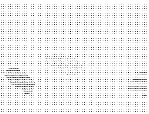
[image:4.612.304.550.65.250.2]We provide simulation results when the proposed algorithm is ap-plied in the “Hamburg taxi” image sequence. The first and the 20th frames are displayed in Figs. 1 and 2. In the center of a frame from this image sequence a white taxi turns around the corner, a black car moves from left to right while a van moves from right to left. The moving object segmentation as provided by the MRBF network for the first frame is shown in Fig. 3. Its corresponding optical flow is provided in Fig. 4. The segmentation and optical flow parameters are used for the initialization of the tracking algorithm.The occluding and unlabeled regions for the first frame are shown in Fig. 5. They are located at the moving object boundaries according to a small local frame reconstruc-tion probability in (7). The pixels of these regions are classified using the MRBF network parameters. The moving object segmentation re-sulted after this classification is displayed in Fig. 6. After tracking the moving objects as described in Section III, we obtain the segmentation of the 20th frame, as provided in Fig. 7. Six past frames(M = 6) have been used for tracking. It can be observed that the segmentation of the white taxi in the center of the frame is quite good despite the fact that, due to the three-dimensional perspective view, its projection changes
Fig. 2. Twentieth frame of the “Hamburg taxi” image sequence.
Fig. 3. Moving object segmentation.
Fig. 4. The optical flow of the first frame from the “Hamburg taxi” image sequence.
[image:4.612.304.551.283.464.2] [image:4.612.305.549.494.681.2]Fig. 5. Occluding and unlabeled regions.
Fig. 6. Segmentation of the moving objects after appropriately classifying the occluding regions.
Fig. 7. Moving object segmentation after tracking them 20 frames.
[image:5.612.307.552.278.463.2]object velocities, is provided in Fig. 9. The difference between the pre-dicted and the real 20th frame is shown in Fig. 10. We can see from this Figure that many errors in the prediction of the 20th frame are due to
[image:5.612.42.288.280.463.2]Fig. 8. Estimated optical flow of the 20th frame.
Fig. 9. Predicted 20th frame.
Fig. 10. Difference between the predicted and the real 20th frame from the “Hamburg taxi” image sequence.
[image:5.612.307.552.496.678.2] [image:5.612.42.289.507.691.2]Fig. 11. PSNR of the predicted frame in the “Hamburg taxi” image sequence. “–” denotes the PSNR of the proposed tracking algorithm. “- -” represents the PSNR prediction considering the initial MRBF model on4 2 4 pixel blocks. “-.” denotes the PSNR between the actual frame and that used for prediction.
Indy Workstation. The trained network, can be used for those succes-sive frames which match the model according to a criterion [6]. In this case, 95 s are required for segmenting the moving objects and the op-tical flow for 20 frames when using424 pixel blocks. When employing tracking as described in this study, only 68 s are necessary for the same frames using pixel resolution segmentation. In the first case only 3040 vectors had been processed while in the second case their number was 48 640. The segmentation provided by the tracking algorithm is quite good as it can be observed from the experimental results and provides a good basis for prediction-based frame reconstruction. The prediction PSNR of the tracking algorithm is better than when considering the initial MRBF model for segmenting all the frames and assuming just the previous moving object features for reconstruction, as it can be ob-served from Fig. 11.
VI. CONCLUSION
We propose a moving object tracking algorithm derived from the Bayesian theory. The optical flow and the segmentation features are jointly modeled by the MRBF network in the initial stage. The oc-cluding and unlabeled regions are detected and classified appropriately. The proposed algorithm provides good moving object tracking capa-bilities. Such capabilities are used for segmenting and estimating the moving object velocity and segmentation in a future frame. The pro-posed algorithm is employed for frame prediction.
REFERENCES
[1] Y. Altunbasak and A. M. Tekalp, “Occlusion-adaptive, content-based mesh design and forward tracking,” IEEE Trans. Image Processing, vol. 6, pp. 1270–1280, Sept. 1997.
[2] K. J. Bradshaw, I. D. Reid, and D. W. Murray, “The active recovery of 3-D motion trajectories and their use in prediction,” IEEE Trans. Pattern Anal. Machine Intell., vol. 19, pp. 219–224, Mar. 1997.
[3] S. M. Smith and J. M. Brady, “ASSET-2: Real-time motion segmenta-tion and shape tracking,” IEEE Trans. Pattern Anal. Machine Intell., vol. 17, pp. 814–820, Aug. 1995.
[4] J. Weber and J. Malik, “Rigid body segmentation and shape description from dense optical flow under weak perspective,” IEEE Trans. Pattern Anal. Machine Intell., vol. 19, pp. 139–143, Feb. 1997.
[5] A. Kumar, Y. B.-Shalom, and E. Oron, “Precision tracking based on seg-mentation with optimal layering for imaging sensors,” IEEE Trans. Pat-tern Anal. Machine Intell., vol. 17, pp. 182–188, Feb. 1995.
[6] A. G. Bors¸ and I. Pitas, “Optical flow estimation and moving object seg-mentation based on median radial basis function network,” IEEE Trans. Image Processing, vol. 7, pp. 693–702, May 1998.
[7] J. Konrad and E. Dubois, “Bayesian estimation of motion vector fields,” IEEE Trans. Pattern Anal. Machine Intell., vol. 14, pp. 910–927, Sept. 1992.
[8] A. G. Bors¸ and I. Pitas, “Median radial basis function neural network,” IEEE Trans. Neural Networks, vol. 7, pp. 1351–1364, Nov. 1996. [9] V. Vapnik, Estimation of Dependences Based on Empirical Data. New
York: Springer-Verlag, 1982.
[10] B. Widrow and S. D. Stearns, Adaptive Signal Processing. Englewood Cliffs, NJ: Prentice-Hall, 1985.
Tomographic Reconstruction Using Nonseparable Wavelets
Stéphane Bonnet, Françoise Peyrin, Francis Turjman, and Rémy Prost
Abstract—In this paper, the use of nonseparable wavelets for
tomo-graphic reconstruction is investigated. Local tomography is also presented. The algorithm computes both the quincunx approximation and detail coefficients of a function from its projections. Simulation results showed that nonseparable wavelets provide a reconstruction improvement versus separable wavelets.
Index Terms—Local tomography, McClellan transformation,
nonsepa-rable wavelets.
I. INTRODUCTION
Computerized tomography (CT) consists of recovering a function from a set of its projections and relies on the inversion of the Radon transform. According to the nature of the data set, this problem may be ill-posed. The use of wavelets for inverse problems in general, and CT in particular, presents several interesting features to stabilize the inversion process [1]. As a matter of fact, wavelets may bring valuable solutions to the problem of local tomography [2]–[4].
The relationships between the continuous wavelet transform and the Radon transform have first been established in several independent works [5], [6]. Olson was the first to devise a reconstruction scheme from a customized sampling of the Radon transform [2]. Delaney [3] and Rashid-Farrokhi [4] proposed a multiresolution tomographic re-construction algorithm to recover the two-dimensional (2-D) separable discrete wavelet transform (2-D DWT) of the image from its projec-tions, and applied it to local tomography. Both algorithms are based on 2-D wavelets, constructed by tensor products of one-dimensional (1-D) wavelets. The 2-D separable wavelets impose a rectangular tiling of the
Manuscript received December 28, 1998; revised February 27, 2000. S. Bonnet was supported by a grant from Siemens, France. This work is in the scope of the scientific topics of the PRC-GDR ISIS research group of the French National Center for Scientific Research (CNRS). The associate editor coordinating the review of this manuscript and approving it for publication was Prof. William Clem Karl.
S. Bonnet and R. Prost are with CREATIS, CNRS Research Unit, 69621 Villeurbanne Cedex, France (e-mail: [email protected]).
F. Peyrin is with CREATIS, CNRS Research Unit, 69621 Villeurbanne Cedex, France. She is also with ESRF, 38043 Grenoble Cedex, France.
F. Turjman is with CREATIS, CNRS Research Unit, 69621 Villeurbanne Cedex, France. He is also with Hôpital Neurologique, 69500 Bron, France.
Publisher Item Identifier S 1057-7149(00)06139-X.