Recurrent Connectivity Can Account for the Dynamics of Disparity Processing in V1

City, University of London Institutional Repository

Citation

:

Samonds, J.M., Potetz, B.R., Tyler, C. W. and Lee, T.S. (2013). Recurrent

Connectivity Can Account for the Dynamics of Disparity Processing in V1. The Journal of

Neuroscience, 33(7), pp. 2934-2946. doi: 10.1523/JNEUROSCI.2952-12.2013

This is the published version of the paper.

This version of the publication may differ from the final published

version.

Permanent repository link:

http://openaccess.city.ac.uk/9351/

Link to published version

:

http://dx.doi.org/10.1523/JNEUROSCI.2952-12.2013

Copyright and reuse:

City Research Online aims to make research

outputs of City, University of London available to a wider audience.

Copyright and Moral Rights remain with the author(s) and/or copyright

holders. URLs from City Research Online may be freely distributed and

linked to.

City Research Online:

http://openaccess.city.ac.uk/

[email protected]

Systems/Circuits

Recurrent Connectivity Can Account for the Dynamics of

Disparity Processing in V1

Jason M. Samonds,

1

_{Brian R. Potetz,}

2

_{Christopher W. Tyler,}

3

_{and Tai Sing Lee}

1

1_{Center for the Neural Basis of Cognition and Computer Science Department, Carnegie Mellon University, Pittsburgh, Pennsylvania 15213,}2_{Department of}

Electrical Engineering and Computer Science, University of Kansas, Lawrence, Kansas 66045, and3_{Kettlewell Brain Imaging Center,}

Smith-Kettlewell Eye Research Institute, San Francisco, California 94115

Disparity tuning measured in the primary visual cortex (V1) is described well by the disparity energy model, but not all aspects of disparity tuning are fully explained by the model. Such deviations from the disparity energy model provide us with insight into how network interactions may play a role in disparity processing and help to solve the stereo correspondence problem. Here, we propose a neuronal circuit model with recurrent connections that provides a simple account of the observed deviations. The model is based on recurrent connections inferred from neurophysiological observations on spike timing correlations, and is in good accord with existing data on disparity tuning dynamics. We further performed two additional experiments to test predictions of the model. First, we increased the size of stimuli to drive more neurons and provide a stronger recurrent input. Our model predicted sharper disparity tuning for larger stimuli. Second, we displayed anticorrelated stereograms, where dots of opposite luminance polarity are matched between the left- and right-eye images and result in inverted disparity tuning in the disparity energy model. In this case, our model predicted reduced sharpening and strength of inverted disparity tuning. For both experiments, the dynamics of disparity tuning observed from the neuro-physiological recordings in macaque V1 matched model simulation predictions. Overall, the results of this study support the notion that, while the disparity energy model provides a primary account of disparity tuning in V1 neurons, neural disparity processing in V1 neurons is refined by recurrent interactions among elements in the neural circuit.

Introduction

Most research on the neurophysiology of binocular vision in pri-mary visual cortex (V1) has focused on hypotheses generated by the feedforward disparity energy model (Ohzawa et al., 1990). The disparity energy model, however, is unable to fully explain disparity tuning in V1 (Cumming and Parker, 1997;Samonds et al., 2009;Tanabe et al., 2011), and local solutions can fail to find the correct solution of disparity (Chen and Qian, 2004;Read and Cumming, 2007). More recent theoretical and experimental re-search suggests models that include neuronal interactions could provide a more accurate description of disparity tuning and such interactions could facilitate disparity processing to find more re-liable estimates of disparity (Menz and Freeman, 2003;Chen and Qian, 2004; Read and Cumming, 2007; Samonds et al., 2009; Tanabe et al., 2011).

There are two primary characteristics of disparity tuning in V1 that are inconsistent with the disparity energy model that we will

address in this article. First, we previously found that disparity tuning curves evolved over time causing the preferred disparity to be more prominent with respect to nonpreferred disparities (Samonds et al., 2009). The sharpened peak and broadened val-leys of disparity tuning curves over time are inconsistent with the Gabor function of disparity predicted by the disparity energy model (Ohzawa et al., 1990). Second, stimulation with anticor-related stereograms (Julesz and Tyler, 1976) generates inverted disparity tuning curves that have weaker modulation amplitudes than disparity tuning curves that result from standard correlated stereogram (Julesz, 1964) stimulation, although the disparity en-ergy model predicts that the modulation amplitudes should be equal (Cumming and Parker, 1997).

In the present study, we developed a simple single-layer neu-ronal network model with feedforward inputs based on the dis-parity energy model (Ohzawa et al., 1990) and recurrent inputs from neighboring neurons constrained by neurophysiological data (Menz and Freeman, 2004;Samonds et al., 2009). We exam-ined whether or not our model could explain the aforementioned variations of V1 disparity tuning from the disparity energy model and performed two experiments to test model predictions. First, the recurrent model replicated sharpening over time, but it also predicted more pronounced sharpening with larger stereograms because more neurons were driven and therefore a larger number of recurrent inputs were activated. When we increased the aper-ture size of stereograms, progressively sharper tuning was also observed in neurophysiological recordings. Second, the recurrent model produced the observed result that inverted disparity tun-Received June 21, 2012; revised Dec. 7, 2012; accepted Dec. 14, 2012.

Author contributions: J.M.S., B.R.P., C.W.T., and T.S.L. designed research; J.M.S. and B.R.P. performed research; J.M.S. and B.R.P. analyzed data; J.M.S., B.R.P., C.W.T., and T.S.L. wrote the paper.

This work was supported by NIH F32 EY017770, NSF CISE IIS 0713206, NIH R01 EY022247, Air Force Office of Scientific Research (AFOSR) FA9550-09-1-0678, NIH P41 EB001977, and a grant from Pennsylvania Department of Health through the Commonwealth Universal Research Enhancement Program. We appreciate the technical assis-tance provided by Karen McCracken, Ryan Poplin, Matt Smith, Ryan Kelly, and Nicholas Hatsopoulos.

Correspondence should be addressed to Jason M. Samonds, 4400 Fifth Avenue, 115 Mellon Institute, Pittsburgh, PA 15213. E-mail: [email protected].

B. R. Potetz’s present address: Google, Los Angeles, CA 90291. DOI:10.1523/JNEUROSCI.2952-12.2013

ing curves from anticorrelated stereogram stimulation had weaker modulation amplitudes than disparity tuning measured from correlated stereogram stimulation. The model additionally predicted much weaker and negligible sharpening of disparity tuning during anticorrelated stereogram stimulation compared with disparity tuning during correlated stereogram stimulation. This was also confirmed with neurophysiological recordings. Both the reduced modulation amplitudes and reduced sharpen-ing occurred in the model because recurrent inputs were weaker when the peaks of anticorrelated disparity tuning curves for re-currently connected neurons did not line up across spatial scale. Overall, these results provide stronger support that facilitative and suppressive interactions among V1 neurons indeed contrib-ute to disparity processing.

Materials and Methods

Neurophysiological recordings.The data for this study were collected

si-multaneously with data reported in two previous articles where the

de-tails about the specific methods can be found (Samonds et al., 2009,

2012). In brief, two different recording procedures were used on three

rhesus monkeys (Macaca mulatta) that were approved by the

Institu-tional Animal Care and Use Committee of Carnegie Mellon University and are in accordance with the National Institutes of Health Guide for the Care and Use of Laboratory Animals. The first recording procedure used for two monkeys (male and female) used two to eight tungsten-in-epoxy and tungsten-in-glass microelectrodes in a chamber overlying the oper-culum of V1 (Samonds et al., 2009). In the second procedure used on the third monkey (male), we recorded from neurons using a chronically implanted 10⫻10 Utah Intracortical Array (400␮m spacing) inserted to a depth of 1 mm in V1 (Samonds et al., 2012). Spike sorting was used to isolate single units (Samonds et al., 2009,2012).

Dynamic random dot stereograms (DRDS) with 25% density of black (⬍0.1 cd/m2_{) and white (50.7 cd/m}2_{) dots on a mean gray background}

(25.3 cd/m2_{) and a 12 Hz refresh rate were centered on the mean position}

of the receptive fields for the population of neurons determined by both minimum response fields based on bar stimuli (Samonds et al., 2009) and spike-triggered receptive fields based on reverse correlation with white noise stimuli (Kelly et al., 2007). Shutter goggles were used to present images to the left and right eyes separately. Because of the small size of the receptive fields (⬍1 degree) and their tight clustering (highly overlap-ping), all receptive fields were well within the DRDS stimuli. For the varying aperture experiment, the DRDS was presented in a 2-, 3-, or 4-degree diameter aperture. No dots were presented outside of the aper-ture and the aperaper-ture size was constant across all disparities. For the correlated versus anticorrelated DRDS experiment, the aperture had a 3.5-degree diameter. For correlated DRDS, there was 100% correspon-dence between black and white dots in the left- and right-eye images (Julesz, 1964). For anticorrelated DRDS, there was 100% correspon-dence of black dots to white dots, and white dots to black dots, in the left- and right-eye images, respectively (Julesz and Tyler, 1976). Eleven disparities between corresponding dots were tested for both experi-ments:⫾0.94,⫾0.658,⫾0.282,⫾0.188,⫾0.094, and 0 degrees. Because the emphasis in this study was quantifying how binocular disparity tun-ing evolved over time, we only examined the most robust data from our recordings (n⫽184 neurons). The responses of the neurons had to have

highly significant disparity tuning (one-way ANOVA,p⬍0.01) and a

disparity discrimination index (DDI) ⬎0.4 (Prince et al., 2002a;

Samonds et al., 2009).

Model.All units in the model were complex cells with feedforward

inputs determined by the energy model (Ohzawa et al., 1990;Cumming

and DeAngelis, 2001) (Fig. 1, Input). Each cell was given a preferred phase disparity␾d, spatial frequency␴, and receptive field center

loca-tionx₀, y₀. We denote the set of these neuronal tuning parameters by␪⫽ {␾d,␴,x0, y0}. The feedforward input given left and right stimuliXLand

XRwas then given by a sum ofNsimple cell responses, each with

qua-dratic nonlinearities, as follows:

IF共XL,XR兩␪兲 ⫽ 1

N

冘

i⫽1

N

rS共XL,XR兩␪,␾i); (1)

⫽_N1

冘

i⫽1

N

共XL 䡠 RL共x,y兩␪,␾i兲

⫹ XR 䡠 RR共x,y兩␪,␾i兲兲2, (2)

whererSis the response of a simple cell of phase␾iwith left and right

receptive fieldsRLandRR.RLis a Gabor filter centered atx0,y0with

spatial frequency␴and phase␾i⫺(␾d/2). The summand ranges over

two or more quadrature pairs of phase␾i. Thus, the feedforward input

into model complex cells follows the energy model (Ohzawa et al., 1990) and was given by the sum of squared binocular Gabor simple cell responses.

When the input stimulus was a DRDS of uniform disparityd, the

expected value of the feedforward input can be shown to be as follows:

IF共d兩␪兲 ⫽ 1

N

冘

i⫽1

N

2RL

冉

x ⫹

d

2,y

冏

␪,␾i

冊

䡠 RR

冉

x ⫺

d

2,y

冏

␪,␾i

冊

⫹ RL 䡠 RL ⫹ RR 䡠 RR (3)

Using Parseval’s theorem, we see that the terms under the summand in Equation 3 do not depend on␾iorN, and so we can write the following:

IF共d兩␪兲 ⫽ 2RL

冉

x ⫹

d

2,y

冏

␪

冊

䡠 RR

冉

x ⫺

d

2,y

冏

␪

冊

⫹ RL 䡠 RL ⫹ RR 䡠 RR (4)

This feedforward disparity tuning curve can be shown to be

approxi-mately Gabor as a function ofd(although the model does not make this

approximation). The response to anticorrelated DRDS was similar, ex-cept the first term of Equation 4 was negative.

In each simulation, we modeled 32 different preferred disparities␾d

(even increments from⫺␲to␲), eight different preferred spatial

fre-quencies␴(subtending four octaves), and a 21⫻21 grid of spatial

locationsx0andy0, for a total of 112,896 simulated neurons. Because

preferred disparity is not uniformly distributed in V1, we sampled

neu-rons according to empirically observed distributions (Prince et al.,

2002b;Liu et al., 2008;Poole et al., 2010).

-Input Local

Long-range

-Complex

y = x2

Left Right Simple

-Input Local

-Complex

y = x2

[image:3.594.304.541.65.227.2]

Left Right Simple

The neural response at timetis given byr(d, t), using a standard dynamic neural field model:

␶⭸u共d_⭸,_tt兩␪兲 ⫽ ⫺u共d,t兩␪兲 ⫹ IF(d,t兩␪)⫹ w共␪兲 䡠 r共d,t兲;

(5)

r共d,t兩␪兲 ⫽ g共u共d,t兩␪兲兲, (6)

wherer(d, t) is the vector of all current neural activity levels,uis the

membrane potential, andw(␪) denotes the lateral connections into

neuron␪.

The neural static nonlinearitygwas given by the sigmoid function:

g共u兲 ⫽ M

1 ⫹ e

uo⫺3u

M

(7)

withu0chosen to produce a baseline firing rate of 20 spikes per second

(sps), andMchosen to produce a maximum firing rate of 200 sps. In our model simulations, no neural firing rate exceeded 100 sps. Therefore, the

nonlinearitygwas effectively monotonically increasing and always

ex-pansive (⭸g/⭸u⬎0;Fig. 1, small grid in each neuron box). Other expan-sive nonlinearities, such asg(u)⫽u2_{, produced similar results.}

Synaptic weights between neurons were chosen to match our conclu-sions from spike time correlation studies (Samonds et al., 2009): facilita-tive connections were drawn between neurons of similar tuning at the same and nearby spatial locations, and inhibitory connections were drawn between neurons of differing tuning within the same spatial loca-tion. Within a spatial locationx0,y0, the weightW(␪i,␪j) between

neu-ronsiandjwas chosen to be proportional to the Pearson correlation

between the feedforward tuning curves of those two neurons (Fig. 1,

Local). This choice was designed to approximate Hebbian learning be-tween neurons: connections bebe-tween neurons strengthen when their fir-ing patterns correlate. Note, however, that the neural response to a natural stimulus is generally substantially reduced and sparser, with fewer neurons firing, in comparison with the response to DRDS. To emulate this, feedforward tuning curves were thresholded before com-puting neural correlations. Thus,W(␪i,␪j) was determined by the

corre-lation betweenmax(T,IF(d兩␪i)) andmax(T,IF(d兩␪j)), whereTwas set to

the median neural input value. Note that all neurons within a spatial location were interconnected. For example, neurons with differing spa-tial frequencies␴may have facilitative or inhibitory connections, de-pending on whether their tuning curves were positively or negatively correlated. The resulting weight distribution was sharp (excitatory con-nection strength tapered rapidly as two neurons differed in disparity tuning), and was primarily inhibitory (⬎75% of all lateral connections were inhibitory).

Across spatial locations, neurons were connected only if they had

matching disparity and spatial frequency preferences (Fig. 1,

Long-range). All cross-spatial connections were positive, and set by a Gaussian, as follows:

W共␪i,␪j兲⬀e

⫺共共xoi⫺xoj兲2⫹共yoi⫺yoj兲2兲

2␴G2 for共xi,yi兲 ⫽ 共xj,yj兲

and共␴i,␾di兲 ⫽ 共␴j,␾dj兲, (8)

with␴Gset to 1.0.

Quantifying sharpening.Unlike previous studies that used reverse

cor-relation analysis to measure tuning curves from responses to rapidly changing stimuli (Menz and Freeman, 2003;Chen et al., 2005;Xing et al., 2005), we measured tuning curves at various delays from stimulus onset to stimuli presented continuously for one second. A lot of consideration and testing went into our choice of how to quantify the changes (e.g.,

sharpening) of disparity tuning over time (Samonds et al., 2013). We

define a sharp tuning curve as one with mean firing rates that are very informative about the most likely value of the stimulus. Among tuning curves with fixed mean firing rate and amplitude, a rapidly firing cell with a sharp tuning curve conveys more information and describes the input

stimulus more precisely than a rapidly firing cell with a dull tuning curve. We examined fitting a Gabor function to the data, fitting a difference of Gaussians function to the data, calculating the Fourier transform, and calculating sample skewness. All methods including our final selection required that tuning curves were reliably measured and robust over time because we were computing the mean firing rate in 100 ms windows, using 10 – 60 trials for each disparity. That is why we chose strict selection criteria for the data that we analyzed (see above). This is because flat or noisy tuning curves can lead to fits with outlier parameters or outlier results with all the potential methods.

The primary problem with a Gabor function or a Fourier transform is that both methods would be chosen to characterize sharpening assuming that a single frequency component was increasing over time in the dis-parity tuning function (Samonds et al., 2013). That assumption was not the case based on our observations of disparity tuning sharpening over time. The primary peak in the disparity tuning function was increasing in frequency, but the valleys were decreasing in frequency (Samonds et al., 2009).Prince et al. (2002a)also previously noted that their Gabor fits deviated from their data with side flanks that were wider than the peak.

Although a Gabor is the standard function for describing disparity tuning over a diverse population of neurons, an alternative function that is not constrained to a single frequency or bandwidth component, and is therefore ideal for capturing the dynamics of disparity tuning described in the study bySamonds et al. (2009), is the difference of Gaussians. A difference of Gaussians function does not always fit well with particular disparity tuning curves and even in a simplified form still requires us to fit 6 parameters to 11 data points, which like a Gabor function, leaves it highly sensitive to the same problems that we encountered with Gabor fits with parameter initialization and outlier results (Samonds et al., 2013). The difference of Gaussians function, however, did provide good fits for some of our robust examples. Although outliers and noise in parameter estimates from difference of Gaussians fits made it difficult to reliably characterize trends over a population of neurons, at least the trends in our robust examples were consistently reflecting some of the properties of sharpening (Samonds et al., 2013).

To simplify our analysis, we chose a method that required no fits, no parameter initialization, and no interpolation. The statistical measure-ment of the sample skewness is the third standardized momeasure-ment of a distribution and can be computed directly from the mean firing ratesf(d) for each disparitydtested:

y1 ⫽

␮3

␴3 ⫽ 1

N

冘

d⫽1

N

共f共d兲 ⫺ f៮兲3

冉

冑

1

N

冘

d⫽1

N

共f共d兲 ⫺ f៮兲2

冊

3 (9)

The difference of Gaussians positive Gaussian peak width produced the most consistent results from all the other methods we considered and although both the positive Gaussian peak width and skewness capture the primary characteristic of disparity tuning over time (narrowing peak), skewness is less noisy (especially with lower firing rates and over a larger population of neurons) and outlier results are less extreme because the computation is much simpler and more robust to noisy tuning curves. Additionally, skewness produces a stronger result because it is also cap-turing the additional characteristics of disparity tuning such as broaden-ing of negative peaks and suppression of secondary positive peaks (Samonds et al., 2013).

All of the methods described above describe the shape of disparity tuning invariant of the strength of the response. However, none of the methods alone can distinguish between what potential mechanisms ac-tually caused the shape of the tuning curves to change over time (e.g., sharpening). In this study, we used data produced from a recurrent neu-ronal network model that we compared with neural recordings to test whether recurrent connectivity could be the underlying mechanism of sharpening. An alternative source of sharpening could be an expansive output nonlinearity (Ohzawa et al., 1990). An expansive output nonlin-earity would sharpen a tuning curve over time if the mean firing rate was increasing. We attempted to avoid this confound by measuring skewness starting at the peak of the population response (100 ms) over an interval where the mean firing rate of the population decreases.

Results

We developed a neural network model with the straightforward organization of a single layer and recurrent connections among binocular disparity-tuned neurons that represent what has been inferred based on cross-correlation results (Menz and Freeman, 2004;Samonds et al., 2009). The organization includes local pos-itive connections among neurons with similar disparity tuning,

different spatial scales, and overlapping receptive fields (Fig. 1; see also Materials and Methods). There are also local nega-tive connections among neurons with dif-ferent disparity tuning and overlapping receptive fields. And finally, there are dis-tant positive connections among neurons with the same disparity tuning, same spa-tial scale, and with neighboring receptive fields across the visual field. For inputs (time step⫽1), we used tuning curves based on the disparity energy model (Ohzawa et al., 1990). We then compared the dynamics of model disparity tuning curves after applying several iterations of recurrent inputs to the dynamics of dis-parity tuning curves measured from re-cordings in the primary visual cortex of awake, behaving macaques while they fix-ated on DRDS.

Eight spatial frequencies (subtending four octaves) and 32 disparity increments were included in the model. The mean fir-ing rate, disparity units assigned to the model, and the range of disparities and frequencies tested were all matched to what was observed from recordings. Only one model simulation was used, and no additional adjustments were made after running the model. Because the model and recordings provided neurons with a variety of preferred disparities and spatial frequencies, examples were chosen for comparison from the model and record-ings that had similar spatial frequencies and preferred disparities.

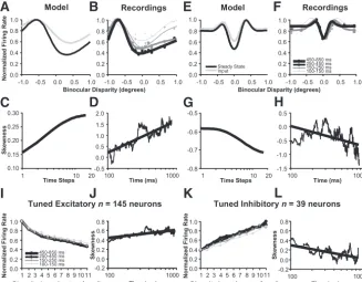
Model captures sharpening of disparity tuning

Model tuning curves and tuning curves measured from record-ings evolved in a similar manner. Peaks became narrower while valleys became wider (Fig. 2A,B) as we reported previously from neurophysiological recordings (Samonds et al., 2009). We quan-tified this behavior with the statistical measurement of the sample skewness of the distribution of mean firing rates over disparity (Eq. 9; see also Materials and Methods) (Samonds et al., 2013). Skewness was measured from recordings using the mean firing rates from 100 ms sliding windows every millisecond. Again, the skewness measured from model data and data from recordings were consistent with each other (Fig. 2C,D) and consistent with our previous observations (Samonds et al., 2009). The skewness increased more strongly in the earliest iterations and during the earliest portion of the neuronal responses soon after the peak of the response onset. The skewness continued to increase over it-erations or time, but at a progressively slower rate. This also happened in the model because the behavior converged to a steady state where the tuning curves no longer changed with a greater number of iterations. Therefore, throughout this article, and as we have done previously (Samonds et al., 2009), we will present all skewness measurements versus log-time-steps (log-iterations) or log-time, and we computed tuning curves from recordings over time using progressively larger windows of time (50, 100, 200, and 400 ms) starting soon after the peak of the response onset in the population (100 ms). For the model, we will compare the input (disparity energy model) and steady-state

tun-0.0 0.2 0.4 0.6 0.8 1.0

-1.0 -0.5 0.0 0.5 1.0

No

rmal

iz

e

d

F

iri

n

g

Rat

e

0.0 0.2 0.4 0.6 0.8 1.0

-1.0 -0.5 0.0 0.5 1.0

10 20

Time (ms) 1000 -0.5

0.0 0.5 1.0 1.5 2.0

100 0.10

0.15 0.20 0.25 0.30

1

Time Steps

B

D

A

C

S

kew

n

ess

Binocular Disparity (degrees)

Model Recordings

0.0 0.2 0.4 0.6 0.8 1.0

-1.0 -0.5 0.0 0.5 1.0 450-850 ms 250-450 ms 150-250 ms 100-150 ms

E

G

F

H

Time (ms)

Model Recordings

Time Steps 0.0

0.2 0.4 0.6 0.8 1.0

-1.0 -0.5 0.0 0.5 1.0 Input

Steady State

100 1000

-1.5 -1.0 -0.5 0.0 0.5

-0.8 -0.7 -0.6 -0.5

1 10 20

Binocular Disparity (degrees)

Tuned Excitatory n= 145 neurons

0.0 0.2 0.4 0.6 0.8 1.0

1 2 3 4 5 6 7 8 9 10 11

No

rmal

iz

e

d

F

iri

n

g

Rat

e

450-850 ms 250-450 ms 150-250 ms 100-150 ms

-0.2 0.8

100 1000

0.0 0.2 0.4 0.6

Sk

e

w

n

e

s

s

Tuned Inhibitory n= 39 neurons

0.0 0.2 0.4 0.6 0.8 1.0

1 2 3 4 5 6 7 8 9 10

No

rmal

iz

e

d

F

iri

n

g

Rat

e

Sk

e

w

n

e

s

s

-0.2 0.0 0.2 0.4 0.6 0.8

100 1000

Time (ms) Time (ms)

Disparity (most-least preferred) Disparity (most-least preferred) 11

J

[image:5.594.46.374.65.320.2]

I

K

L

ing curves (result of the final iteration). For the recordings, we will compare the tuning curve measured from the initial window of time to subsequent windows of time from response onset. Our initial window is still delayed and therefore would likely include some sharpening from recurrent interactions so it is possible that some changes in actual neurons are happening faster than we can measure them.

Skewness can vary substantially depending on the preferred disparity and spatial frequency of a neuron. For model neurons, the skewness varied from⫺1.5 to 3.0 for our sample of tuning curves, which is consistent with the variation that we observed in the actual neurons as well. The model does also produce variation in temporal dynamics (some neurons converge to a steady-state faster than other neurons) depending on the preferred disparity and spatial frequency. For actual neurons, the skewness measure-ments tended to be too noisy in individual cases, making it im-practical to systematically compare their skewness convergence with the variations in convergence behaviors in model neurons. The direction of change of skewness over time, however, did not vary in the model. Overall, the examples of different preferred disparities and spatial frequencies that we present throughout this article are representative of the variety of behavior observed in the model and recordings.

Disparity tuning dynamics for tuned inhibitory neurons In models, binocular disparity-tuned neurons that are classified as tuned inhibitory (Poggio and Fischer, 1977;Poggio et al., 1988) do not behave in the same manner as tuned excitatory neurons, especially with respect to an expansive output nonlinearity (Read et al., 2002;Haefner and Cumming, 2008). We initially separated our disparity tuned neurons into tuned inhibitory and tuned excitatory categories to test for differences in behavior in the model and neurophysiological recordings. Neurons were classi-fied as tuned inhibitory when they had one primary negative peak and two positive peaks that were not significantly different ( Sa-monds et al., 2012), and our population of 184 disparity-tuned neurons described in this article included 39 (21%) tuned inhib-itory neurons. The primary difference we observed in the model, and for the neurophysiological data, is that features of sharpening were inverted for tuned inhibitory neurons with respect to tuned excitatory neurons: the primary negative peak narrowed and be-came more prominent, and skewness decreased over time.

Figure 2(top right panels) demonstrates the disparity tuning dynamics for an example tuned inhibitory model and recorded neuron. Over time, the primary negative peaks became narrower and more prominent with respect to other disparities (Figs. 2E, black vs gray;F, black vs progressively lighter curves). The change in shape over time was confirmed by showing that the skewness was decreasing at an approximately linear rate versus log-time-steps and log-time (Fig. 2G,H, respectively).

We summarize the inverted behavior of tuned inhibitory neu-rons (primary negative peak,n⫽39 neurons) with respect to tuned excitatory neurons (primary positive peak,n⫽145 neu-rons) in the bottom row ofFigure 2. We sorted tuning curves from the most- to the least-preferred ranked disparity based on the primary positive peak or negative peak, respectively, before averaging. For tuned excitatory neurons, the responses to non-preferred disparities became relatively weaker over time com-pared with the response to the preferred disparity in the population average tuning curve (Fig. 2I). Additionally, the av-erage skewness increased at an approximately linear rate versus log-time (Fig. 2J). For tuned inhibitory neurons, responses to nonpreferred disparities (based on the primary negative peak)

became relatively stronger (farther away in mean firing rate dif-ference) over time compared with the response to the preferred disparity in the population average tuning curve (Fig. 2K). As in the examples, for tuned inhibitory neurons, the average skewness decreased at an approximately linear rate versus log-time (Fig. 2L). Overall, the behavior was very similar between the two sub-populations, but inverted with respect to each other when based on tuning shape, sharpening, and skewness. Results were very similar for alternative criteria in dividing neurons into the tuned excitatory and tuned inhibitory classes, such as the ratio of posi-tive peak height (maximum⫺mean) compared with negative peak height (mean⫺minimum). Since the average behavior of tuned inhibitory neurons was consistently inverted for both the aperture size and anticorrelated versus correlated DRDS experi-ments, we inverted their tuning curves and skewness measure-ments for any population analysis described in subsequent sections, and we confirm the consistency of the inversion in the final section. Because these neurons only represent 21% of the population, even if we did not invert these tuning curves, the general observation was that during DRDS stimulation with cor-related DRDS using a DRDS with a large aperture (⬎3 degrees), disparity tuning sharpened and skewness versus log-time had a significantly average positive slope (p⬍0.02).

Model predictions

To conduct a stricter test of whether or not recurrent interactions like those incorporated into our model could predict the dynam-ics of disparity tuning observed in our recordings, we examined the dynamics of disparity tuning in the model and from record-ings while applying more complex manipulations to DRDS stim-uli. First, we examined the disparity tuning dynamics while increasing the size of the DRDS, therefore covering a greater number of receptive fields and exciting a greater number of neu-rons. Then we compared the disparity tuning dynamics between traditional stereograms (Julesz, 1964) and anticorrelated stereo-grams (Julesz and Tyler, 1976), where the input tuning curve ends up inverted in the disparity energy model (Cumming and Parker, 1997).

Disparity tuning dynamics depend on DRDS aperture size When neurons in primary visual cortex are driven by progres-sively larger drifting sinusoidal luminance gratings with varying orientation, the orientation tuning curves exhibit progressively more sharpening (Chen et al., 2005;Xing et al., 2005). Because the size of these gratings in these studies extended well beyond the classical receptive field and the orientation tuning sharpened over time, this result suggests that the larger gratings were recruit-ing a larger number of recurrent inputs that had a delayed and increasingly stronger contribution to orientation tuning. We tested for whether similar behavior occurred for binocular dis-parity tuning in our model and recordings with DRDS with pro-gressively larger apertures.

We first inspected the steady-state tuning curves in the model and tuning curves of individual neurons in the latest part of the stimulation period analyzed and compared the curves computed from responses to DRDS with varying aperture size.Figure 3,A

curves were sharper for the responses to DRDS with larger aper-tures (Fig. 3, light gray curves).

Next, we looked at how the disparity tuning curves sharpened over time for varying DRDS aperture size for the model and recordings.Figure 4,AandF, shows the input and initially mea-sured (100 –150 ms after stimulus onset) normalized tuning curves for an example neuron in the model and recordings, re-spectively. For the model, the input tuning curves for the three DRDS aperture sizes were exactly the same (Fig. 4A), and for the recordings, the tuning curves for the three DRDS aperture sizes were very similar (Fig. 4F).Figure 4,BandG, shows the steady state and latest measured (450 – 850 ms after stimulus onset) tun-ing curves for the same neuron in the model and recordtun-ings, respectively. They reveal that over multiple iterations (or time), the response was relatively weaker to nonpreferred disparities compared with the preferred disparity, and the peaks became narrower for larger DRDS aperture sizes (increasingly lighter curves). This change in shape can be more clearly illustrated by plotting the skewness of the distribution of mean firing rates in the tuning curve over multiple iterations or over time. The skew-ness for both the model disparity tuning and disparity tuning measured from the recorded neuron increased more for larger DRDS aperture sizes (Fig. 4E,J) compared with smaller DRDS aperture sizes (Fig. 4C,H).

We summarized the behavior observed inFigure 4by com-puting a population average of normalized disparity tuning and skewness over time steps or time for model neurons and recorded neurons for varying DRDS aperture sizes (Fig. 5). The responses were sorted with respect to ranked disparity from the most pre-ferred to least prepre-ferred before averaging. As in the examples, for the population average of normalized disparity tuning over time, the responses were relatively weaker to nonpreferred disparities compared with the preferred disparity for DRDS stimulation with the largest aperture size, revealing a clear change in shape (Fig. 5C,K, black vs light gray). As aperture size increased, you can clearly see that the response to the least preferred disparity

be-came relatively weaker or closer to the dashed line. This change in shape was confirmed by observing a greater increase in average skewness versus log-time for DRDS stimulation with the largest aperture size (Fig. 5G,O) compared with DRDS stimulation with the smallest aperture size (Fig. 5E,M). For each recorded neuron (n⫽81), we performed linear regression on the normalized fir-ing rate versus log-disparity rank for the disparity tunfir-ing mea-sured in the latest response window (i.e., a log-fit for the black curves inFig. 5I–K). The average fall-off rate in relative mean firing rate with progressively more nonpreferred disparities (Fig. 6A) was significantly larger for the 4-degree DRDS aperture size versus the 2- and 3-degree DRDS aperture size (p⬍0.001), and the 3-degree DRDS aperture size versus the 2-degree DRDS ap-erture size (p⬍0.05). Therefore, the response to the preferred disparity became significantly more prominent with increasing size of a DRDS aperture. Additionally, for each recorded neuron, we performed linear regression on skewness versus log-time. The average slope of the fit increased with DRDS aperture size (Fig. 6B) and was significantly positive (p⬍0.01) and greater for a DRDS with a 4-degree aperture size versus a DRDS with a 2-degree aperture size (p⬍0.05). Therefore, disparity tuning sharpened more with increasing size of a DRDS aperture.

Although skewness is invariant with respect to changes in the mean and variance of the tuning curve (see Materials and Meth-ods), it cannot distinguish sharpening caused by recurrent inter-actions versus sharpening caused by an increase in mean firing rate over time coupled with an expansive output nonlinearity, which is part of the disparity energy model (e.g., squaring the response) (Ohzawa et al., 1990). We attempted to avoid this con-found by measuring skewness starting at the peak of the popula-tion response (100 ms) over an interval where the mean firing rate of the population decreases. To confirm whether or not this was true, we performed linear regression on the mean firing rate versus log-time (Fig. 5P), and the mean firing rate significantly decreased over the interval that we measured skewness for DRDS stimulation with all three aperture sizes (p⬍0.001). Finally, we also examined the mean firing rate with aperture size (Figs. 5L, 6C) since skewness increased with aperture size. The average mean firing rate (Fig. 6C) significantly decreased with increasing aperture size (p⬍0.001) so the sharpening we observed cannot be explained by an expansive output nonlinearity alone and is incompatible with the disparity energy model. The decrease in mean firing rate with increasing aperture size additionally sup-ports that the increased DRDS aperture size is recruiting a greater number of recurrent inputs outside of the classical receptive field rather than simply increasing the excitatory input to the classical receptive field.

Disparity tuning dynamics for correlated versus anticorrelated DRDS

In a traditional DRDS, there is 100% correspondence or correla-tion between the left and right-eye images (Julesz, 1964). Each black and white dot in the left-eye image has a matching black and white dot, respectively, in the right-eye image, but all shifted at the same horizontal disparity. Neurons with binocular disparity tuning in V1 also respond selectively to anticorrelated DRDS (Cumming and Parker, 1997), where each black (and white) dot in the left-eye image has a matching white (and black) dot, re-spectively, in the right-eye image that are at the same horizontal disparity (inverted polarity) (Julesz and Tyler, 1976). However, the observed modulation amplitude of the inverted disparity tun-ing curve for anticorrelated DRDS is weaker than the disparity tuning curve for correlated DRDS (Cumming and Parker, 1997;

2 degrees 3 degrees 4 degrees

Model Recordings

size 1 size 2 size 3

Binocular Disparity (degrees)

0 10 20 30

-1.0 -0.5 0.0 0.5 1.0

0 5 10 15

-1.0 -0.5 0.0 0.5 1.0 20

B

0 10 20 30 40 50

-1.0 -0.5 0.0 0.5 1.0

0 10 20 30 40 50

-1.0 -0.5 0.0 0.5 1.0

A

Firi

ng R

a

te

(

s

ps

[image:7.594.45.283.63.265.2]

)

Ohzawa et al., 1997;Nieder and Wagner, 2001). The disparity energy model pre-dicts that the tuning between the two stimuli will be inverted, but have equal strength in modulation (Eq. 4). To try to explain this discrepancy, we examined the tuning curves measured from the re-sponses to correlated and anticorrelated DRDS for both model and neurophysio-logical data (n⫽103 neurons). We used the measurement of skewness to reveal and compare the dynamics of disparity tuning for correlated and anticorrelated DRDS stimuli for our model and neuro-physiological data.

Examples of the model data (Fig. 7A) and data from recordings (Fig. 7B) illustrate that the tuning curves based on anticorlated DRDS (gray) were inverted with re-spect to correlated DRDS (black) as predicted by the disparity energy model and as reported previously (Cumming and Parker, 1997). Both the model results and data from recordings had tuning curves for anticorrelated DRDS with smaller modulation amplitudes than tun-ing curves for correlated DRDS. Popula-tion averages of tuning curves were generated by sorting the data from the most preferred disparity to the least pre-ferred ranked disparity (both based on correlated DRDS) before averaging. These population averages show that the in-verted tuning for anticorrelated DRDS stimulation was consistent across the populations (Fig. 7C,D). The reduced modulation amplitude for our population of tuning curves based on anticorrelated DRDS stimulation (Fig. 7F,n⫽103,␮⫽ 0.60) was also consistent with previous re-ports (Cumming and Parker, 1997; Ohzawa et al., 1997;Nieder and Wagner, 2001). However, our model with recur-rent interactions also replicated the

re-duced modulation amplitude for anticorrelated DRDS

stimulation (␮ ⫽ 0.63, although with a narrower and more skewed distribution;Fig. 7E), so our model could explain this phenomenon that is not predicted if disparity tuning is modeled with the disparity energy model alone (Cumming and Parker, 1997).

Applying a threshold (Eq. 7) to a disparity energy model neu-ron can produce reduced modulation amplitude for anticorre-lated DRDS stimulation without any recurrent interactions among disparity-tuned neurons (Lippert and Wagner, 2001). However, the threshold only reduces the modulation amplitude for tuned excitatory neurons and actually increases the modula-tion amplitude for tuned inhibitory neurons (Read et al., 2002). Nonetheless, because there are more tuned excitatory neurons (n⫽82) than tuned inhibitory neurons (n⫽21) (Prince et al., 2002b;Liu et al., 2008;Poole et al., 2010), a threshold alone could still result in an average amplitude modulation ratio of less than one. Our model also replicated this bias (see Materials and Meth-ods) so the threshold in our model indeed produced an initial

(before any recurrent interactions) average amplitude modula-tion ratio that is less than one (␮⫽0.84). However, previous studies have observed no systematic relationship between ampli-tude modulation ratio and phase disparity (Nieder and Wagner, 2001) and there are clear examples of amplitude modulation ra-tios of less than one for tuned inhibitory neurons (Cumming and Parker, 1997). For our neurophysiological data, we did observe that the amplitude modulation ratio is slightly higher for tuned inhibitory neurons (n⫽21,␮⫽0.66) versus tuned excitatory neurons (n⫽82,␮⫽0.58), but the amplitude modulation ratio was still far below one for tuned inhibitory neurons and the dif-ference between the populations was not statistically significant (p⫽0.27). Although the recurrent interactions in our model did substantially reduce the amplitude modulation ratio from␮⫽ 0.84 to␮⫽0.63, the amplitude modulation ratio of tuned inhib-itory neurons was still higher than the amplitude modulation ratio of tuned excitatory neurons. However, we could reduce and produce amplitude modulation ratios significantly below one for tuned inhibitory neurons by adjusting the balance between the

0.0 0.2 0.4 0.6 0.8 1.0

-1.0 -0.5 0.0 0.5 1.0

2 degrees 3 degrees 4 degrees 100-150 ms 450-850 ms 0.0 0.2 0.4 0.6 0.8 1.0

-1.0 -0.5 0.0 0.5 1.0

Normal iz ed Fir ing R a te

Binocular Disparity (degrees) -1.5 -1.0 -0.50.0 0.5 1.0 1.5 100 1000 2 degrees -1.5 -1.0 -0.50.0 0.5 1.0 1.5 Ske w n e

ss 3 degrees

100 1000 -1.5 -1.0 -0.50.0 0.5 1.0 1.5 Time (ms) 100 1000 4 degrees

F

G

H

I

J

0.0 0.2 0.4 0.6 0.8 1.0

-1.0 -0.5 0.0 0.5 1.0

size 1 size 2 size 3 Input Steady State 0.0 0.2 0.4 0.6 0.8 1.0

-1.0 -0.5 0.0 0.5 1.0

Norm al iz ed Fir in g R a te

Binocular Disparity (degrees)

size 1 Ske w n e ss size 2 Time Steps size 3

A

B

C

D

E

1.4 1.5 1.6 1.7

1 10 20

1.4 1.5 1.6 1.7

1 10 20

1.4 1.5 1.6 1.7

1 10 20

Model Recordings

Figure 4. Disparity tuning dynamics for neurons when stimulated by DRDS with increasing aperture sizes.A,B, Example early and late tuning curves from the model for varying aperture size, respectively.C–E, Example skewness measurements from the model for increasing aperture size.F,G, Example early and late tuning curves from recordings for varying aperture size, respec-tively.H–J, Example skewness measurements from recordings for increasing aperture size.

n = 81 neurons 2 degrees 0.0 0.2 0.4 0.6 0.8 1.0

1 2 3 4 5 6 7 8 91011

Normal iz ed Fir in g R a te 250-450 ms 150-250 ms 100-150 ms

I

1000 0.0 0.2 0.4 0.6 0.8 100 3 degrees

J

Ske w n e ss 0.0 0.2 0.4 0.6 0.8 1.0

1 2 3 4 5 6 7 8 91011

K

0 5 10 15 20 25 30

1 2 3 4 5 6 7 8 91011 Disparity (most-least preferred)

2 degrees 3 degrees 4 degrees 1000 0.0 100 0.0 0.2 0.4 0.6 0.8 1.0

1 2 3 4 5 6 7 8 91011 4 degrees 0 5 10 15 20 25 30 100 Time (ms) 1000 0.0 100 1000

L

M

N

O

P

0.0 0.2 0.4 0.6 0.8 1.0 1 32 Input Steady State 450-850 ms 0.0 0.2 0.4 0.6 0.8 1.0 1 32 0.0 0.2 0.4 0.6 0.8 1.0 1 32 Normal iz ed Fir ing R a te 0 10 20 30 40 50 1 32 size 1 size 2 size 3

Disparity (most-least preferred) 0.0

1 10 20

0.0

1 10 20

0.0

1 10 20

0.2 0.4 0.6 0.8 0.2 0.4 0.6 0.8 0.2 0.4 0.6 0.8 0.2 0.4 0.6 0.8 Ske w n e ss Model Recordings 0 10 20 30 40

1 10 20

Time Steps

A

B

C

D

E

F

G

H

F ir in g Ra te (s ps) Firi ng R a te ( s ps ) size 1 size 2 size 3

Tuning Skewness Tuning Skewness

[image:8.594.215.541.64.197.2]

0.2 0.4 0.6 0.8

threshold and the recurrent interactions in the model. Because the threshold increases amplitude modulation and the recurrent interactions reduce amplitude modulation, this was accom-plished by relatively weakening the threshold (a more gradual increase in rate or smaller exponent) and/or strengthening the recurrent input.

Not only was the modulation amplitude generally weaker for anticorrelated compared with correlated DRDS, but the shape of the disparity tuning curves differed between the stimuli as well. We inspected the steady-state tuning curves in the model and tuning curves of individual neurons in the latest part of the stim-ulation period analyzed and compared the curves computed from responses to correlated DRDS to the curves computed from responses to anticorrelated DRDS.Figure 8,AandC, shows dis-parity tuning curves measured from the responses to correlated and anticorrelated DRDS for two example model neurons and two recorded neurons, respectively. The tuning curves measured from anticorrelated DRDS stimulation were not simply inverted tuning curves measured from correlated DRDS with weaker modulation amplitudes. To illustrate this more clearly, we nor-malized the tuning curves by the peak response and inverted the tuning curve measured from the response to anticorrelated DRDS (Fig. 8B,D, dashed line and open circles, respectively). Tuning curves measured from correlated DRDS had narrower peaks and broader valleys, and secondary peaks were relatively suppressed compared with what we observed in anticorrelated DRDS tuning curves. The responses to nonpreferred disparities were relatively much weaker compared with the preferred dispar-ities for tuning curves measured from the responses to correlated versus anticorrelated DRDS. Overall, the tuning curves were sharper for the responses to correlated DRDS compared with anticorrelated DRDS.

Next, we looked at how model tuning curves and tuning curves measured from responses to correlated and anticorrelated DRDS sharpened over time (Fig. 9).Figure 9,AandC, shows how

example normalized tuning curves for a neuron in the model and recordings, respectively, change over time when presented a standard correlated DRDS. Over multiple iterations or time, the response was relatively weaker to nonpreferred disparities compared with the preferred disparity. Peaks became narrower and valleys became wider. This change in shape can be more clearly illustrated by plotting the skewness of the tuning curve over multiple iterations or over time. The skewness for both the model disparity tuning curve and disparity tuning curve mea-sured from the recorded neuron increased at an approximately linear rate versus log-time-step (iteration) and log-time, respec-tively (Fig. 9B,D). Although the tuning curves measured from anticorrelated DRDS stimulation of the same model neuron and example recorded neuron (Fig. 9E,G) also changed over time in relative magnitude at different disparities, the shape did not ap-pear to change as much and the tuning curve did not sharpen in the same consistent manner as during correlated DRDS stimula-tion. This qualitative observation was confirmed with the skew-ness measurement over iterations or time (Fig. 9F,H) by revealing no clear increase and consistent change in the skewness of disparity tuning during anticorrelated DRDS stimulation.

We summarized the behavior observed inFigure 9by com-puting a population average of normalized disparity tuning and skewness over time steps or time for model neurons and recorded neurons during correlated and anticorrelated DRDS stimulation

**

*

***

*

_***

***

-0.30 -0.25 -0.20 -0.15 -0.10 -0.05 0.00

Nor

malized

F

iri

ng

Rate

lo

g-rank-dis

parit

y

-0.05 0.00 0.05 0.10 0.15

Ske

w

ness/log-ti

me

***

0 5 10 15 20 25

2 degrees 3 degrees 4 degrees

M

e

a

n

Fi

ri

ng R

a

te

(

s

p

s

)

A

B

C

* p< 0.05 ** p< 0.01 *** p< 0.001

Figure 6. Summary of population statistical tests of disparity tuning dynamics for neurons when stimulated by DRDS with varying aperture size.A, The fall-off in firing rate (thick black curve,Fig. 10I–K) is faster for nonpreferred disparities for larger apertures.B, The skewness of disparity tuning curves increases more rapidly for larger apertures.C, The mean firing rate decreases for larger aper-tures showing that there is surround suppression during DRDS stimulation.

0 10 20 30 40 50

1 2 3 4 5 6 7 8 9 10 11

Disparity (most-least preferred)

Firi

ng R

a

te

(

s

ps

)

DRDS a-DRDS

0 10 20 30 40 50 60

DRDS a-DRDS

2 3 1

0 0.1 0.2 0.3 0.4

0.0 0.4 0.8 1.2 1.6

Ratio of

#

of N

e

urons

0 0.1 0.2 0.3 0.4

0.0 0.4 0.8 1.2 1.6

Modulation Amplitude Ratio (a-DRDS/DRDS)

Model Recordings

0 20 40 60

-1.0 0.0 1.0

Firi

ng R

a

te

(

s

ps

)

10 30 50

Binocular Disparity (degrees)

0 20 40 60 80

-1.0 0.0 1.0

B

D

A

C

F

E

n = 103 neurons

disparity energy model disparity

energy model recurrent model

expansive output nonlinearity

[image:9.594.306.540.64.352.2]

only

(Fig. 10). The responses were sorted with respect to ranked disparity from the most preferred to least preferred (both based on DRDS stimulation) before averaging. As in the examples, for the population aver-age of disparity tuning over time, the

re-sponses were relatively weaker to

nonpreferred disparities compared with the preferred disparity for DRDS stimula-tion with a clear change in shape (Fig. 10A,C, black vs light gray), which was confirmed by observing that the average skewness increased at an approximately linear rate versus log-time (Fig. 10B,D). During anticorrelated DRDS stimulation, there was some relatively weakened re-sponse for nonpreferred disparities com-pared with the preferred disparity for model neurons in the population average (Fig. 10E), but less than what was ob-served during DRDS stimulation (Fig. 10A). Also, there was almost no noticeable change in shape of the population average of disparity tuning during anticorrelated DRDS stimulation, which was confirmed by observing little change in skewness over time steps (Fig. 10F). Any changes in disparity tuning measured from anticor-related DRDS were even less clear in the population averages of the responses to recorded neurons (Fig. 10G,H). For each recorded neuron (n ⫽ 103), we per-formed linear regression on skewness ver-sus log-time. The average slope of the fit was significantly positive (p⬍0.001) for correlated DRDS stimulation and was sig-nificantly greater for correlated DRDS

versus anticorrelated DRDS stimulation (p⬍0.01).

To again rule out the possibility that increasing skewness was solely the result of sharpening caused by an expansive output nonlinearity, we also performed linear regression on the mean firing rate versus log-time. For the model and this experiment, the overall mean firing rate was stronger for disparity tuning measured from the responses to correlated versus anticorrelated DRDS stimuli (Fig. 7C,D), so with an expansive output nonlin-earity, we predicted that disparity tuning would be overall sharper for correlated versus anticorrelated DRDS stimulation. Indeed, the initial skewness measurements are higher for the re-sponses to correlated versus anticorrelated DRDS (Fig. 10B, vsF,

DvsH). However, the expansive output nonlinearity does not predict that the skewness would increase for either condition over time because the mean firing rate significantly decreased over the interval that we measured skewness for both correlated (p⬍

0.001) and anticorrelated (p⬍0.05) DRDS stimulation. Addi-tionally, if we sample tuning curves for correlated and anticor-related DRDS stimulation so that they have equal distribution of tuning strength (based on DDI), the slope measurements are nearly identical to the measurements based on all neurons:n⫽29 neurons, 0.10 (p⫽0.10) versus⫺0.03 (p⫽0.58) skewness/log-time for correlated versus anticorrelated DRDS stimulation. This supports that the tuning curves measured from anticorrelated DRDS stimulation are not sharpening over time even when they have the same tuning strength as curves measured during

corre-lated DRDS stimulation. Overall, the sharpening we observed over time for the responses to correlated DRDS cannot be plained by stronger mean firing rates, stronger tuning, or an ex-pansive output nonlinearity.

Even though the statistical tests of the population averages reveal a significant decrease in mean firing rate over time during the interval where we measured skewness, there is diversity in how the mean firing rate evolves over time for individual neurons and for some neurons, the mean firing rate continually increases over time (Samonds et al., 2009). Therefore, we examined the slopes of skewness and mean firing rate versus log-time to make sure that particular extreme examples did not disproportionately contribute to any particular significant trends of skewness over time that we observed. The vast majority of the strong increases of skewness over time coincided with decreases in mean firing rate over time and for the small number of examples where both skewness and mean firing rate increased over time, the mean firing rate increased proportionally less than when mean firing rates decreased over time. We note that in the study bySamonds et al. (2009), even in those examples where skewness was increas-ing and mean firincreas-ing rate was continually increasincreas-ing, there were still features of sharpening over time that could not be explained by an expansive output nonlinearity, such as suppressed second-ary peaks. Overall, there was no significant correlation between how skewness or mean firing rate varied over time (r⫽0.00,

p⫽0.97).

N o rma li z e d Fi ri ng R a te 0 10 20 30 40 50

-1.0 -0.5 0.0 0.5 1.0

0 10 20 30 40 50

-1.0 -0.5 0.0 0.5 1.0 0.0 0.2 0.4 0.6 0.8 1.0

-1.0 -0.5 0.0 0.5 1.0

B

Model 0.0 0.2 0.4 0.6 0.8 1.0

-1.0 -0.5 0.0 0.5 1.0

Binocular Disparity (degrees)

Fi ri n g R a te (s ps ) 0.0 0.2 0.4 0.6 0.8 1.0

-1.0 -0.5 0.0 0.5 1.0

a-DRDS (inverted) 0.0 0.2 0.4 0.6 0.8 1.0

-1.0 -0.5 0.0 0.5 1.0

D

0 5 10 15 20 25

-1.0 -0.5 0.0 0.5 1.0

C

Recordings

-1.0 -0.5 0.0 0.5 1.0

Binocular Disparity (degrees)

[image:10.594.216.543.284.396.2]

DRDS a-DRDS N o rma li z e d Fi ri ng R a te 0 20 40 60 80 Fi ri n g R a te (s ps)

A

a-DRDS (inverted) DRDS a-DRDS

Figure 8. Disparity tuning curves measured from neurons stimulated by correlated DRDS are sharper than tuning curves measured from the same neurons when stimulated by anticorrelated DRDS (a-DRDS). All tuning curves were measured using the last iteration (steady-state) or latest block of time analyzed following stimulus onset (450 – 850 ms).A, Example tuning curves from the model.B, Peak response-normalized tuning curves fromA.C, Example tuning curves from recordings.D, Peak response-normalized tuning curves fromC. Error bars inCare SE with respect to trials.

0.0 0.2 0.4 0.6 0.8 1.0

-1.0 -0.5 0.0 0.5 1.0

450-850 ms 250-450 ms 150-250 ms 100-150 ms 0.0 0.2 0.4 0.6 0.8 1.0

-1.0 -0.5 0.0 0.5 1.0 Binocular Disparity (degrees)

Normal iz ed Fir ing R a te -1.0 -0.5 0.0 0.5 1.0 1.5 Time (ms) -1.0 -0.5 0.0 0.5 1.0 1.5 Ske w n e ss 100 1000 100 1000

C

G

D

H

Model Recordings 0.0 0.2 0.4 0.6 0.8 1.0

-1.0 -0.5 0.0 0.5 1.0

Input Steady State 0.0 0.2 0.4 0.6 0.8 1.0

-1.0 -0.5 0.0 0.5 1.0 Binocular Disparity (degrees)

-0.1 0.0 0.1 0.2 0.3 0.4 0.5

1 10 20

Ske w n e ss Normal iz ed Fir ing R a te -0.1 0.0 0.1 0.2 0.3 0.4 0.5

1 10 20 Time Steps DRDS a-DRDS

A

E

B

F

Figure 9. Disparity tuning dynamics for neurons when stimulated by correlated (DRDS) versus anticorrelated DRDS (a-DRDS).A,

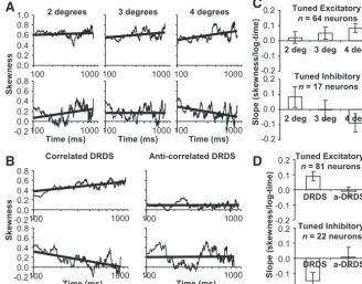
Disparity tuning dynamics for both experiments for tuned inhibitory neurons

To verify that the behavior was consistently inverted for tuned inhibitory neurons with respect to tuned excitatory neurons, we examined the results for each experiment on the subpopulations separately. As we increased the size of the DRDS aperture, there were greater increases in skewness for tuned excitatory neurons (Fig. 11A,C, top row, left-to-right) and greater decreases in skew-ness for tuned inhibitory neurons (Fig. 11A,C, bottom row, left-to-right). We also compared the changes in skewness measured for excitatory and inhibitory tuned neurons while changing from correlated to anticorrelated DRDS stimulation. During corre-lated DRDS stimulation, the skewness increased for tuned excit-atory neurons (Fig. 11B,D, top row) and decreased for tuned inhibitory neurons (Fig. 11B,D, bottom row). During anticorre-lated DRDS stimulation there was no clear change in skewness over time for both tuned excitatory neurons (Fig. 11B,D, top row) and tuned inhibitory neurons (Fig. 11B,D, bottom row). Overall, these results support that the behavior of tuned excit-atory neurons and tuned inhibitory neurons are consistent with each other for the two experiments, but inverted with respect to the direction of change for skewness.

Recurrent network versus a feedforward network

To deconstruct the contributions of the expansive output non-linearity, the disparity tuning-dependent connectivity, and re-currence in our network, we measured disparity tuning dynamics for two simple feedforward networks and compared these results to our recurrent network results.

For the first feedforward model, recurrent connections were removed from the original model except for self connections to simulate neural dynamics. This resulted in a feedforward model where only the expansive output nonlinearity could produce sharpening of disparity tuning over time. Because the mean firing rate increased slightly over time in this feedforward model, there was only a small amount of sharpening (⬍1% increase in skew-ness) over time and a small reduction in the amplitude modula-tion ratio from correlated to anticorrelated DRDS stimulamodula-tion only because of the greater ratio of tuned excitatory versus tuned inhibitory neurons (Fig. 7E).

For the second feedforward model, we retained the lateral connections in our original model so that they were still consis-tent with disparity tuning-dependent connectivity between neu-rons (Menz and Freeman, 2004;Samonds et al., 2009). However, recurrence was removed so that the remaining lateral connec-tions occurred only in one direction. In other words, we removed

[image:11.594.45.374.64.166.2]

the connections at all but one neuron, measured the response of that neuron, and then repeated this procedure for each of the neurons in our population. This ef-fectively modified our recurrent network into a feedforward model with an addi-tional layer of neurons. For the original layer, we had disparity energy neurons representing all possible preferred dispar-ities and spatial frequencies in our model. These neurons then provided inputs to an equal amount of neurons (representing all possible preferred disparities and spatial frequencies) with weighting equivalent to our original lateral connections. One way to visualize this would be to consider that the center neuron in the local circuit in Figure 1represents an example neuron in the new layer, while all neurons connected to this center neuron represent example neu-rons in the original layer. The difference in the multilayer feed-forward version of our model with respect to the recurrent model inFigure 1was that all connections from the center neuron in the new layer back to the surrounding neurons in the original layer were no longer present.

In the original full model with both the expansive output linearity and recurrent connections, sharpening due to the non-linearity and sharpening due to recurrent connections interact with each other significantly. If we remove either the nonlinearity or the recurrent connections, we end up with less sharpening. Without recurrence, the multilayer feedforward model still had 56% of the increase in skewness compared with the recurrent model suggesting that our lateral connections implemented in a feedforward manner alone could account partly for the observa-tion of sharpened disparity tuning. Indeed, previous feedforward models of disparity tuning in V1 have replicated sharpening be-havior such as suppressed secondary peaks (Tanabe et al., 2011). However, the mean firing rate increased more substantially over time for our multilayer feedforward model while the mean firing rate decreased over time for the recurrent model, so we cannot rule out that some of the remaining sharpening might have been caused by the expansive output nonlinearity in this feedforward model. Additionally, although the weighted inputs or the expan-sive output nonlinearity in the multilayer feedforward model alone can produce some proportion of the overall sharpening observed, the recurrent model provides the simplest explanation of the slowly increasing skewness over time, especially consid-ering that the observed mean firing rate of recordings was decreasing. Furthermore, the weighted inputs in the multilayer feedforward model did not replicate the aperture size experiment results and only produced negligible differences (⬍1%) in the modulation amplitude reduction between correlated and anti-correlated DRDS stimulation beyond what resulted from apply-ing the expansive output nonlinearity alone (Fig. 7E). Overall, our model required the weighted inputs between disparity-tuned neurons to circulate through recurrent connections to gain any significant power. An alternative feedforward model than the one we tested could potentially replicate more of the steady-state be-havior of our recurrent model given enough freedom of com-plexity and number of layers. What makes the recurrent model a more appealing explanation, however, is the simplicity of requir-ing only a srequir-ingle recurrent layer and that the model captures both the steady-state and dynamic behavior that we observed in neu-rophysiological recordings.

450-850 ms 250-450 ms 150-250 ms 100-150 ms

Time (ms) 1000

n = 103 neurons 0.0

0.2 0.4 0.6 0.8 1.0

1 2 3 4 5 6 7 8 9 1011

Norm

al

iz

ed Fir

ing

R

a

te

1000 -0.2

0.0 0.2 0.4 0.6 0.8

100

Ske

w

n

e

ss

0.0 0.2 0.4 0.6 0.8 1.0

1 2 3 4 5 6 7 8 9 1011 -0.2 0.0 0.2 0.4 0.6 0.8

100

D

H

Model Recordings

C

G

Input Steady State

0.0 0.2 0.4 0.6 0.8 1.0

1 32

Norm

al

iz

ed Fir

ing

R

a

te

Disparity (most-least preferred) 0.0

0.2 0.4 0.6 0.8 1.0

1 32

Disparity (most-least preferred) DRDS

a-DRDS 0.0 0.2 0.4 0.6 0.8

1 10 20

Time Steps

Ske

w

n

e

ss

0.0 0.2 0.4 0.6 0.8

1 10 20

B

F

A

E