This is a repository copy of
Light scattering from solid-state quantum emitters: Beyond the
atomic picture
.
White Rose Research Online URL for this paper:
http://eprints.whiterose.ac.uk/145085/
Version: Submitted Version
Article:
Brash, A.J. orcid.org/0000-0001-5717-6793, Iles-Smith, J., Phillips, C.L. et al. (8 more
authors) (Submitted: 2019) Light scattering from solid-state quantum emitters: Beyond the
atomic picture. arXiv. (Submitted)
© 2019 The Author(s). For reuse permissions, please contact the Author(s).
[email protected] https://eprints.whiterose.ac.uk/ Reuse
Items deposited in White Rose Research Online are protected by copyright, with all rights reserved unless indicated otherwise. They may be downloaded and/or printed for private study, or other acts as permitted by national copyright laws. The publisher or other rights holders may allow further reproduction and re-use of the full text version. This is indicated by the licence information on the White Rose Research Online record for the item.
Takedown
If you consider content in White Rose Research Online to be in breach of UK law, please notify us by
Alistair J. Brash,1,∗ Jake Iles-Smith,1, 2,† Catherine L. Phillips,1 Dara P. S. McCutcheon,3 John O’Hara,1
Edmund Clarke,4 Benjamin Royall,1 Jesper Mørk,5 Maurice S. Skolnick,1 A. Mark Fox,1 and Ahsan Nazir2
1Department of Physics and Astronomy, University of Sheffield, Sheffield, S3 7RH, United Kingdom
2School of Physics and Astronomy, The University of Manchester, Oxford Road, Manchester M13 9PL, UK
3Quantum Engineering Technology Labs, H. H. Wills Physics Laboratory and Department
of Electrical and Electronic Engineering, University of Bristol, Bristol BS8 1FD, UK
4EPSRC National Epitaxy Facility, Department of Electronic and Electrical Engineering, University of Sheffield, Sheffield, UK
5Department of Photonics Engineering, DTU Fotonik,
Technical University of Denmark, Building 343, 2800 Kongens Lyngby, Denmark
(Dated: April 12, 2019)
Coherent scattering of light by a single quantum emitter is a fundamental process at the heart of many proposed quantum technologies. Unlike atomic systems, solid-state emitters couple to their host lattice by phonons. Using a quantum dot in an optical nanocavity, we resolve these interactions in both time and frequency domains, going beyond the atomic picture to develop a comprehensive model of light scattering from solid-state emitters. We find that even in the presence of a cavity, phonon coupling leads to a sideband that is completely insensitive to excitation conditions, and to a non-monotonic relationship between laser detuning and coherent fraction, both major deviations from atom-like behaviour.
Scattering of light by a single quantum emitter is one of the fundamental processes of quantum optics. First ob-served in atomic systems [1, 2], and more recently studied extensively in self-assembled quantum dots (QDs) [3–6], coherent scattering attracts interest as the scattered light retains the coherence of the laser rather than the emit-ter. As such, their coherence may exceed the conven-tional radiative limit whilst still exhibiting antibunch-ing on the timescale of the emitter lifetime [3–6]. Ex-ploiting this behaviour gives rise to exciting possibili-ties for quantum technologies such as generating tune-able single photons [7–9], realising single photon non-linearities [10–14], and constructing entangled states be-tween photonic [15, 16] or spin [17, 18] degrees of freedom. For a continuously driven emitter, coherent scatter-ing occurs in the weak excitation regime where absorp-tion and emission become a single coherent event. For a simple two-level“atomic picture”with only spontaneous emission and pure dephasing, the coherently scattered fraction (FCS) of the total emission is given by [19]:
FCS=
T2
2T1
1
1 +S, (1)
where S = (Ω2T
1T2)/(1 + ∆2LXT22) is a generalized
sat-uration parameter, Ω is the Rabi frequency, ∆LX =
ωL −ωX is the detuning between the laser (ωL) and
the emitter (ωX) and T1 and T2 are the emitter
life-and coherence times respectively. It is clear from this expression that the fraction of coherently scattered light reaches unity in the limit of driving well below saturation (S ≪1) and transform-limited coherence (T2= 2T1).
Solid-state emitters (SSEs), particularly self-assembled QDs, are an attractive system with which to realise such schemes owing to their high brightness and ease of inte-gration with nanophotonic structures. However, unlike
atoms, SSEs can experience significant dephasing from fluctuating charges [20, 21] and coupling to vibrational modes of the host material [22, 23]. Despite this, state-of-the-art InGaAs QD single photon sources have demon-strated essentially transform-limited photons emitted via the zero phonon line (ZPL) [24–26] through careful sam-ple optimisation, exploitation of photonic structures and by using resonantπ-pulse excitation at cryogenic temper-atures. Although these results show ZPL broadening can be effectively suppressed, coupling to vibrational modes also leads to the emergence of a phonon sideband (PSB) in the emission spectrum [23, 27–31]. This is attributed to a rapid change in lattice configuration of the host ma-terial during exciton recombination, leading to the simul-taneous emission or absorption of longitudinal acoustic (LA) phonons with the emission of a photon [27, 28, 32]. Therefore, to obtain perfectly indistinguishable photons the PSB must be filtered out, naturally limiting the ef-ficiency of the device, even when using an optical cavity to Purcell enhance emission into the ZPL [31, 33].
The aforementioned works [23, 27–31, 33] have revealed the importance of phonon coupling in the incoherent regime, where there is a definite change of charge config-uration in the QD, such that incoherently scattered reso-nance fluorescence dominates the spectrum. It is perhaps natural to presume that phonon coupling may be elim-inated by operating in the coherent scattering regime, since there is vanishing exciton population and therefore no change in charge configuration. This suggests that, in accordance with most works in the literature [3–5], one may adopt the atom-like picture of Eq. 1, where the coherent fraction tends towards unity for excitation far below saturation and transform-limited coherence. How-ever, a recent theoretical study predicted that PSBs oc-cur even for vanishingly weak resonant driving [30].
2
0.1 1 10 100 1000
0.0 0.8 0.9 1.0
Experiment Polaron ME Pure Dephasing
F
ri
n
g
e
co
n
tra
st
Time (ps)
-2 -1 0
10-3
10-2
10-1
100 Experiment Polaron ME
In
te
n
si
ty
(a
.u
.)
Detuning (meV) SPAD
SPAD
Liquid He T= 4.2 K
Laser
FPI
50:50 BS Signal
LP 50:50
BS LP
CCD
Mach-Zehnder Interferometer Spectrometer
QD
nm
SM Fiber
Diverter Mirror
[image:3.612.58.558.51.223.2](b) (a)
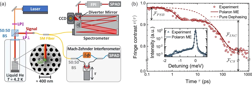
FIG. 1. (a) Schematic of the experiment: BS - beam splitter, CCD - charge-coupled device (camera), FPI - Fabry-Perot interferometer, LP - linear polarizer, SM - single mode fiber, SPAD - single photon avalanche diode, ∆φ - phase shift, τ
- path length difference. (b) Measurement of the first-order correlation function (g(1)(τ)) atS = 0.25 with ∆
LX = 0. The
emission contains phonon sideband (FP SB), incoherent resonance fluorescence (FI N C) and coherently scattered (FCS) fractions.
Experimental measurements of fringe contrast (red circles) agree well with a calculation using the polaron master equation (solid red line) where the phonon coupling strengthαand cut-off frequencyνcare the only free parameters. A pure dephasing
model (dashed red line) decays mono-exponentially and cannot capture phonon dynamics. Inset: An experimental spectrum (blue triangles) measured simultaneously is also well reproduced by the polaron model (blue line) with the same parameters. The calculated spectrum is convolved with the spectrometer instrument response in order to reproduce the observed ZPL width.
Here, we experimentally verify that PSBs persist in the coherent scattering regime and demonstrate additionally that phonon processes also cause large deviations from atom-like physics when driving off-resonance. An ex-tended theoretical model fully describes our solid-state nanocavity system, providing an intuitive picture that at-tributes the PSB to phonon dressing of the optical dipole moment. This leads to a finite probability that the vibra-tional environment changes state during an optical scat-tering event, implying that all optical spectral features will have an associated PSB. Whilst a self-assembled QD is studied here, we emphasize that the physics and meth-ods apply equally to a diverse range of SSEs, including vacancy centers in diamond [34, 35], defects in hexagonal boron nitride [36], monolayer transition metal dichalco-genides [37] and single carbon nanotubes [38].
To study this phonon coupling experimentally, we in-vestigate a neutral exciton state (|Xi) of a self-assembled InGaAs QD with dipole moment |~µ| = 27.2 D, weakly coupled (~g= 135µeV) to a H1 photonic crystal cavity (linewidth ~κ= 2.51 meV) with Purcell factorFP = 43
(see Ref. [26] for full details). As well as Purcell en-hancing the ZPL, the cavity also acts as a weak spectral filter; this combination can reduce the PSB component of the emission [31, 33], motivating the coupling of SSEs to cavities. Fig. 1(a) illustrates the experiment; the sample is held in a liquid helium bath cryostat at T = 4.2 K and excited by a tuneable laser that is rejected from the detection path by cross-polarisation (typical signal-to-background>100:1). The coherence of the scattered light is studied either in the time domain by measuring
the fringe contrastv(τ) in a Mach-Zehnder interferome-ter or in the frequency domain using a spectromeinterferome-ter or a Fabry-Perot interferometer (FPI) for higher resolution (details in supplemental material (SM) [39]).
It is instructive to begin with a high resolution time-domain measurement, exciting resonantly below satura-tion (S = 0.25) where coherent scattering is expected to dominate the emission. The measured fringe con-trast v(τ) is proportional to the first order correlation function g(1)(τ) [39]. The result in Fig. 1(b) departs
significantly from the mono-exponential radiative decay predicted by atomic theory (dashed line); a rapid decay of coherence occurs in the first few picoseconds, compa-rable to phonon dynamics observed in pulsed four-wave mixing measurements of InGaAs QDs in the incoherent regime [40], suggesting that the rapid loss of coherence we observe originates from electron-phonon interactions. In order to describe such behaviour accurately, we must account for the microscopic nature of the QD-phonon coupling [41]. This is achieved by applying the polaron transformation to the full system-environment Hamiltonian, dressing the excitonic states of the system with modes of the phonon environment. We may then derive a master equation (ME) that is non-perturbative in the electron-phonon coupling strength [30, 42–44] to describe the evolution of the reduced state of the QD [39]. In the polaron frame, the first-order cor-relation function is gpol(1)(τ) = G(τ)g(1)opt(τ) [30], where
g(1)opt(τ) is the purely optical contribution found using
the correlation function of the phonon environment, which accounts for non-Markovian phonon relaxation. Here we have defined the phonon propagator ϕ(τ) = αR∞
0 νe
−ν2
/ν2
c(cos(ντ) coth(ν/2kBT)−isin(ντ))dν, and the Franck-Condon factorB = exp(−ϕ(0)/2). The cou-pling of the QD to the phonon environment is thus speci-fied by its thermal energykBT, the deformation potential
coupling strengthα, and cut-off frequencyνc[27, 41, 45].
The cavity leads both to Purcell enhancement of the ex-citon transition (included within the ME) and spectral filtering of the emission. We incorporate cavity filtering by solving the Heisenberg equations of motion for the cavity field operators, leading to the detected function:
gD(1)(τ) = Z ∞
−∞ ˜
h(t−τ)g(1)pol(t)dt, (2)
where ˜h(t) = exp(−i∆XCt−κ|t|/2) is the cavity filter
function and ∆XC is the exciton-cavity detuning [39].
By fitting the phonon bath correlation function con-tained within Eq. 2 to the first few picoseconds of the measurement, we extract phonon parameters α = 0.0447 ps2andν
c= 1.28 ps−1, comparable to values
pre-viously found for InGaAs QDs [46]. Using experimentally determined values for all other parameters, we accurately reproduce the full dynamics of the experimental data, as shown by the solid line in Fig. 1. After phonon relax-ation, radiative decay associated with incoherent reso-nance fluorescence occurs between τ = 20−200 ps. Fi-nally, atτ≫200 ps,v(τ) plateaus, corresponding to the coherent fraction of the emission. As the laser coherence time is much greater than the measured delays, no de-cay of the coherent scattering is observed. From thev(τ) amplitudes, we extract FPSB = 0.06, FINC = 0.14 and
FCS= 0.80 respectively for the PSB, incoherent and
co-herent fractions of the total emission (F). Crucially, a finiteFPSBunder weak driving indicates that Eq. 1 does
not fully describe the scattering dynamics of the system. To check the accuracy of the extracted parameters we now move to the frequency domain. The theoretical spec-trum is calculated by Fourier transforming g(1)D (τ) and may be written as: S(ω) = H(ω)(Sopt(ω) +SSB(ω)),
where H(ω) = (κ/2)/[(ω−∆XC)2+ (κ/2)2] is the
fre-quency domain cavity filter function [31, 47, 48]. The spectrum consists of two principal components: a purely optical part
Sopt(ω) =B2
Z ∞
−∞
gopt(τ)eiωτdτ, (3)
containing both coherent and incoherent contributions to the spectrum, and a second incoherent component
SSB(ω) =
Z ∞
−∞ G
(τ)−B2
gopt(τ)eiωτdτ, (4)
which gives rise to the PSB [30, 31]. The ZPL contri-bution is thus reduced by the square of the constant
Franck-Condon factorB2, with the missing fraction
emit-ted through the PSB.
The inset to Fig. 1 illustrates that the parameters ex-tracted from the time domain dynamics lead to excellent agreement between the experimental (blue triangles) and theoretical (S(ω) - solid line) spectra, with a broad PSB observed in accordance with the short timescale of the phonon processes. These combined time and frequency domain measurements provide critical insight into the na-ture of electron-phonon interactions in driven QDs: even well below saturation, where the excited state popula-tion is small and coherent scattering dominates, a PSB is present, comprising∼6% of the emission.
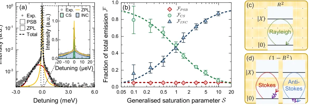
To investigate to what extent the PSB persists in the coherent scattering regime, we measure the resonance flu-orescence spectrum as a function of saturation by varying Ω. Fig. 2(a) shows a spectrum taken well above satu-ration (S = 10) that exhibits a ZPL (yellow fit) and a PSB (SSB(ω) - red fit). Performing high resolution
spec-troscopy of the ZPL with the FPI results in the inset to Fig. 2(a) which exhibits a broad contribution from in-coherent resonance fluorescence (blue fit) and a narrow feature from coherent scattering (green fit). As in the g(1)(τ) of Fig. 1(b), the total spectrum thus comprises
three components whose fraction of the total emission can be evaluated from their areas (details in [39]).
Fig. 2(b) shows the evolution of the components of the resonant (∆LX= 0) scattering spectrum as a function of
S. The polaron model agrees well with the experiment and produces a curve forFCS (green dashed line) that
is proportional to (1 +S)−1 like Eq. 1. However, as
previously predicted [30], FCS does not reach unity for
vanishingS, a surprising result that may be explained by observing that the PSB fraction FP SB (red diamonds)
is constant and independent of Ω. This contrasts with excitation induced dephasing (EID) [46, 49] which is also mediated by LA phonons and captured within our model, but is proportional to (Ω2+ ∆2
LX) and is thus negligible
for resonant driving below saturation.
4 |0 | Rayleigh (1 ) |0 | Anti-Stokes (c) (d) Stokes
0.05 0.1 0.2 0.5 1 2 5 10 20
0.0 0.2 0.4 0.6 0.8 1.0
-3.0 0.0 3.0 6.0
10-3 10-2 10-1 100 In te n si ty (a .u .) Detuning (meV) Exp. PSB ZPL Total (a)
-20 -10 0 10 20 0.0 0.5 1.0 In te n si ty (a .u .)
Detuning ( eV) Exp. ZPL CS INC F ra ct io n o f to ta l e mi ssi o n
[image:5.612.63.559.53.224.2]Generalised saturation parameter (b)
FIG. 2. Components of the resonant scattering spectrum. (a) Semi-log spectrum at low resolution (S = 10, ∆LX= 0): grey
circles - experiment; yellow - fit to ZPL; red - fit to PSB; black dashed line - total fit. Inset: High resolution spectrum: grey circles - experiment; green - fit to coherent scattering; blue - fit to incoherent resonance fluorescence; yellow - total fitted profile. (b) Evolution with increasing Ω: red diamonds - PSB; green circles - coherent scattering; blue triangles - incoherent resonance fluorescence; dashed lines - polaron model. (c) Coherent scattering occurs when laser photons scatter directly from the bare transition (solid black lines) with probability given by the square of the Franck-Condon factor (B2). (d) Inelastic scattering
occurs when the system scatters (with probability (1−B2)) into a different vibrational state within the ground-state manifold
(grey shading). An LA phonon (purple) is emitted or absorbed for the Stokes and anti-Stokes cases respectively.
emergence of a PSB. At low bath temperatures, phonon absorption is suppressed, resulting in the characteristic asymmetry of the PSB. From Eqs. 3 and 4, the branch-ing ratio between phonon-mediated inelastic and elastic scattering is determined solely by the constantB2.
Out-side the Mollow triplet regime, the coherent (S ≪1) and incoherent (S &1) resonant scattering spectra of a SSE thus differ only in the width of the ZPL. As such, whilst coherent scattering is often cited as a route to highly co-herent single photons, it cannot negate the PSB.
To gain further insight into phonon interactions in the scattering picture, the effect of detuning the laser from the emitter is now considered. Fig. 3(a) shows semi-log plots of spectra taken at constant Ω with laser detun-ing~∆LX =±0.27 meV. The coherent peaks at ~∆LX
are separated from the ZPL and dominate the spectrum. For positive detuning (blue spectrum), it is immediately noticeable that the high-energy edge of the sideband is shifted by ∼ ~∆LX. The origins of this behaviour can
be seen in Eq. 4, where the product betweengopt(1)(τ) and
(G(τ)−B2) in the time-domain implies a convolution in
frequency between the purely optical spectrum and the frequency-space phonon correlation function. As such, all optical features inSopt have an associated PSB; the
coherent peak (and thus its PSB) shifts with ∆LX.
The-oretically (Fig. 3(a) inset), the low-energy edge of the sideband would also be expected to shift for negative de-tuning (red spectrum); experimentally this is obscured by weak incoherent backgrounds owing to the low count-rate at large ∆LX. The total PSB fraction is still governed
byB2: since sideband processes arise from phonon
dress-ing of the optical transition, they apply equally to both coherent and incoherent peaks, irrespective ofωL.
Further deviations from the conventional atomic pic-ture can be seen in the balance of coherent and in-coherent scattering when driving off-resonance. Com-pared to the experiment, both the atomic and polaron theories significantly over-estimate the coherent fraction away from resonance (details in SM [39]). We attribute this to the Lorentzian reduction in QD absorption with |∆LX|, allowing laser light to instead be absorbed in
the doped bulk material [50], leading to charge noise. To capture the associated pure dephasing in both the atomic and polaron models, we include a Lorentzian detuning-dependent dephasing rateγ(∆LX) withγ(0) =
0, γ(∆LX → ∞) = γmax and width fixed to the QD
linewidth [39]. By fitting the polaron theory to the data we findγmax= 21±0.1µeV. Spectral wandering is then accounted for by convolving with a Gaussian noise func-tion with width deduced from the incoherent peak ob-served in detuned spectra (Fig. 3(a)) [39].
In Fig. 3(b), upper and lower bounds (from uncer-tainty in Ω) of the atomic (green curves) and polaron (red curves) models are plotted. Experimental values ofFCS
(grey circles) are evaluated as in Fig. 1(b). In stark con-trast to the atomic theory, where Eq. 1 predictsFCSwill
only ever increase with |∆LX|, the measured data only
increases close to resonant driving where EID [46, 49] is small. For |∆LX| between 0.1 and 0.4 meV, this EID
-2 -1 0 1 2 3 10-4 10-3 10-2 10-1 100 N o rma lise d in te n si ty Detuning (meV) : +0.27 meV -0.27 meV (a) 0.27 meV
-0.8 -0.4 0.0 0.4 0.8
0.0 0.2 0.4 0.6 C o h e re n t fra ct io n
Laser detuning (meV)
(b)
Experiment Atomic Model Polaron ME -2 -1 0 1 2
[image:6.612.57.561.52.222.2]10-3 10-1 101 In te n s it y (a .u .) Detuning (meV) |0 | > 0 (c) |0 | < 0 (d) Rayleigh Inc. Rayleigh
FIG. 3. Phonon influences in detuned (∆LX6= 0) coherent scattering. (a) Semi-log spectra (normalised by integrated intensity)
for ∆LX =±0.27 meV (blue/red) at constant ~Ω = 5.7 µeV. Inset: Theoretical spectrum. (b)FCS vs. ∆LX at constant
~Ω = 25.6µeV: grey circles - experimentalFCS extracted as in Fig. 1(b); red lines polaron master equation; green lines
-atomic model, both models include additional pure dephasing and spectral wandering [39] and have upper and lower bounds from uncertainty in Ω. (c) For ∆LX>0, emission of an LA phonon can populate|Xi, allowing incoherent relaxation. (d) For
∆LX<0, populating|Xirequires LA phonon absorption which is weak atT = 4.2 K.
resonance (∆LX >0) as in Fig. 3(c), |Xican be
pop-ulated through the emission of an LA phonon [51–53] (purple arrow), increasing the probability of incoherent scattering (orange arrow). When ∆LX <0 (Fig. 3(d)),
populating |Xiis inhibited at T = 4.2 K as it requires phonon absorption [54, 55], inhibiting incoherent scatter-ing. For ∆LX <−0.5 meV, the probability of phonon
absorption becomes sufficiently low thatFCS begins to
increase again towards the limiting atomic case. This behaviour deviates strongly from the atomic model and requires careful consideration for schemes involving de-tuned coherent scattering, such as generating single [8, 9] or entangled [15, 16] photons.
In conclusion, we have shown that a fixed fraction of light scattered from a solid-state emitter is always lost through a phonon sideband, irrespective of excita-tion condiexcita-tions such as Rabi frequency or detuning. We have also demonstrated that the detuning dependence of the coherent fraction is strongly modified by the pres-ence of phonon coupling, contradicting the atomic pre-diction that the coherent fraction will increase monoton-ically with detuning. Both processes can be intuitively understood by considering phonon-dressing of the opti-cal transition of the QD. Taken together, these results illustrate the importance of employing an appropriate model of phonon coupling rather than assuming atom-like physics when driving weakly or off-resonance. For example, treating phonons in a crude pure-dephasing approximation (e.g. Eq. 1), suggests they may be sup-pressed simply by increasing the Purcell factor. This is directly contradicted by the clear separation of phonon and radiative timescales in Fig. 1(b), with the phonon sideband persisting despite a large Purcell enhancement.
The methods developed here can be used to optimise quantum information protocols such as spin-photon en-tanglement schemes for realistic solid-state emitters.
This work was funded by the EPSRC (UK) EP/N031776/1, A.N. is supported by the EPSRC (UK) EP/N008154/1 and J.I.S. acknowledges support from the Royal Commission for the Exhibition of 1851. Note: Af-ter the completion of our experiments, we became aware of related results [56]. We thank B.D. Gerardot for bring-ing these to our attention.
∗ Email: [email protected] † Email: [email protected]
[1] H. M. Gibbs and T. N. C. Venkatesan, Direct observa-tion of fluorescence narrower than the natural linewidth, Optics Communications17, 87 (1976).
[2] J. Volz, M. Weber, D. Schlenk, W. Rosenfeld, C. Kurt-siefer, and H. Weinfurter, An atom and a photon, Laser Physics17, 1007 (2007).
[3] H. S. Nguyen, G. Sallen, C. Voisin, P. Roussignol, C. Diederichs, and G. Cassabois, Ultra-coherent sin-gle photon source, Applied Physics Letters 99, 261904 (2011).
[4] C. Matthiesen, A. N. Vamivakas, and M. Atat¨ure, Sub-natural linewidth single photons from a quantum dot, Phys. Rev. Lett.108, 093602 (2012).
[5] R. Proux, M. Maragkou, E. Baudin, C. Voisin, P. Rous-signol, and C. Diederichs, Measuring the photon coales-cence time window in the continuous-wave regime for res-onantly driven semiconductor quantum dots, Phys. Rev. Lett.114, 067401 (2015).
6
and A. J. Shields, Cavity-enhanced coherent light scatter-ing from a quantum dot, Science Advances 10.1126/sci-adv.1501256 (2016).
[7] C. Matthiesen, M. Geller, C. H. H. Schulte, C. Le Gall, J. Hansom, Z. Li, M. Hugues, E. Clarke, and M. Atature, Phase-locked indistinguishable photons with synthesized waveforms from a solid-state source, Nat. Communica-tions4, 1600 (2013).
[8] Y. He, Y.-M. He, Y.-J. Wei, X. Jiang, M.-C. Chen, F.-L. Xiong, Y. Zhao, C. Schneider, M. Kamp, S. H¨ofling, C.-Y. Lu, and J.-W. Pan, Indistinguishable tunable single photons emitted by spin-flip raman transitions in ingaas quantum dots, Phys. Rev. Lett.111, 237403 (2013). [9] T. M. Sweeney, S. G. Carter, A. S. Bracker, M. Kim, C. S.
Kim, L. Yang, P. M. Vora, P. G. Brereton, E. R. Cleve-land, and D. Gammon, Cavity-stimulated raman emis-sion from a single quantum dot spin, Nat. Photonics 8, 442 (2014).
[10] A. Javadi, I. Sllner, M. Arcari, S. L. Hansen, L. Midolo, S. Mahmoodian, G. Kiransk, T. Pregnolato, E. H. Lee, J. D. Song, S. Stobbe, and P. Lodahl, Single-photon non-linear optics with a quantum dot in a waveguide, Nat. Communications6, 8655 (2015).
[11] A. Sipahigil, R. E. Evans, D. D. Sukachev, M. J. Bu-rek, J. Borregaard, M. K. Bhaskar, C. T. Nguyen, J. L. Pacheco, H. A. Atikian, C. Meuwly, R. M. Ca-macho, F. Jelezko, E. Bielejec, H. Park, M. Lonˇcar, and M. D. Lukin, An integrated diamond nanophotonics plat-form for quantum optical networks, Science 10.1126/sci-ence.aah6875 (2016).
[12] A. J. Bennett, J. P. Lee, D. J. P. Ellis, I. Farrer, D. A. Ritchie, and A. J. Shields, A semiconductor photon-sorter, Nat. Nanotechnology11, 857 (2016).
[13] L. De Santis, C. Ant´on, B. Reznychenko, N. Somaschi, G. Coppola, J. Senellart, C. G´omez, A. Lemaˆıtre, I. Sagnes, A. G. White, L. Lanco, A. Auff`eves, and P. Senellart, A solid-state single-photon filter, Nat. Nan-otechnology 12, 663 (2017).
[14] D. Hallett, A. P. Foster, D. L. Hurst, B. Royall, P. Kok, E. Clarke, I. E. Itskevich, A. M. Fox, M. S. Skolnick, and L. R. Wilson, Electrical control of nonlinear quan-tum optics in a nano-photonic waveguide, Optica5, 644 (2018).
[15] E. V. Denning, J. Iles-Smith, D. P. S. McCutcheon, and J. Mork, Protocol for generating multiphoton entangled states from quantum dots in the presence of nuclear spin fluctuations, Phys. Rev. A96, 062329 (2017).
[16] D. Scerri, R. N. E. Malein, B. D. Gerardot, and E. M. Gauger, Frequency-encoded linear cluster states with co-herent raman photons, Phys. Rev. A98, 022318 (2018). [17] A. Delteil, Z. Sun, W.-b. Gao, E. Togan, S. Faelt, and A. Imamolu, Generation of heralded entanglement be-tween distant hole spins, Nature Physics12, 218 (2015). [18] R. Stockill, M. J. Stanley, L. Huthmacher, E. Clarke, M. Hugues, A. J. Miller, C. Matthiesen, C. Le Gall, and M. Atat¨ure, Phase-tuned entangled state generation be-tween distant spin qubits, Phys. Rev. Lett. 119, 010503 (2017).
[19] Eq. 1 generalises expressions from C. Cohen-Tannoudji, J. Dupont-Roc, and G. Grynberg, Atom-Photon Inter-actions: Basic Processes and Applications (Wiley-VCH, 1998) pp. 369,383 to include pure dephasing.
[20] J. Houel, A. V. Kuhlmann, L. Greuter, F. Xue, M. Pog-gio, B. D. Gerardot, P. A. Dalgarno, A. Badolato,
P. M. Petroff, A. Ludwig, D. Reuter, A. D. Wieck, and R. J. Warburton, Probing single-charge fluctuations at a GaAs/AlAs interface using laser spectroscopy on a nearby ingaas quantum dot, Phys. Rev. Lett.108, 107401 (2012).
[21] A. V. Kuhlmann, J. Houel, A. Ludwig, L. Greuter, D. Reuter, A. D. Wieck, M. Poggio, and R. J. Warburton, Charge noise and spin noise in a semiconductor quantum device, Nat. Physics9, 570 (2013).
[22] E. A. Muljarov and R. Zimmermann, Dephasing in quan-tum dots: Quadratic coupling to acoustic phonons, Phys. Rev. Lett.93, 237401 (2004).
[23] A. Reigue, J. Iles-Smith, F. Lux, L. Monniello, M. Bernard, F. Margaillan, A. Lemaitre, A. Martinez, D. P. S. McCutcheon, J. Mørk, R. Hostein, and V. Vo-liotis, Probing electron-phonon interaction through two-photon interference in resonantly driven semiconductor quantum dots, Phys. Rev. Lett.118, 233602 (2017). [24] N. Somaschi, V. Giesz, L. De Santis, J. C. Loredo,
M. P. Almeida, G. Hornecker, S. L. Portalupi, T. Grange, C. Antn, J. Demory, C. Gmez, I. Sagnes, N. D. Lanzillotti-Kimura, A. Lematre, A. Auffeves, A. G. White, L. Lanco, and P. Senellart, Near-optimal single-photon sources in the solid state, Nat. Photonics10, 340 (2016).
[25] H. Wang, Z.-C. Duan, Y.-H. Li, S. Chen, J.-P. Li, Y.-M. He, M.-C. Chen, Y. He, X. Ding, C.-Z. Peng, C. Schneider, M. Kamp, S. H¨ofling, C.-Y. Lu, and J.-W. Pan, Near-transform-limited single photons from an effi-cient solid-state quantum emitter, Phys. Rev. Lett.116, 213601 (2016).
[26] F. Liu, A. J. Brash, J. OHara, L. M. P. P. Martins, C. L. Phillips, R. J. Coles, B. Royall, E. Clarke, C. Bentham, N. Prtljaga, I. E. Itskevich, L. R. Wilson, M. S. Skol-nick, and A. M. Fox, High purcell factor generation of indistinguishable on-chip single photons, Nat. Nanotech-nology13, 835 (2018).
[27] B. Krummheuer, V. M. Axt, and T. Kuhn, Theory of pure dephasing and the resulting absorption line shape in semiconductor quantum dots, Phys. Rev. B65, 195313 (2002).
[28] P. Kaer and J. Mørk, Decoherence in semiconductor cav-ity QED systems due to phonon couplings, Phys. Rev. B
90, 035312 (2014).
[29] D. P. S. McCutcheon, Optical signatures of non-markovian behavior in open quantum systems, Phys. Rev. A93, 022119 (2016).
[30] J. Iles-Smith, D. P. S. McCutcheon, J. Mørk, and A. Nazir, Limits to coherent scattering and photon co-alescence from solid-state quantum emitters, Phys. Rev. B95, 201305(R) (2017).
[31] J. Iles-Smith, D. P. S. McCutcheon, A. Nazir, and J. Mørk, Phonon scattering inhibits simultaneous near-unity efficiency and indistinguishability in semiconductor single-photon sources, Nat. Photonics11, 521 (2017). [32] L. Besombes, K. Kheng, L. Marsal, and H. Mariette,
Acoustic phonon broadening mechanism in single quan-tum dot emission, Phys. Rev. B63, 155307 (2001). [33] T. Grange, N. Somaschi, C. Ant´on, L. De Santis, G.
R. G. Beausoleil, Resonant enhancement of the zero-phonon emission from a colour centre in a diamond cav-ity, Nat. Photonics5, 301 (2011).
[35] E. Neu, D. Steinmetz, J. Riedrich-Mller, S. Gsell, M. Fis-cher, M. Schreck, and C. BeFis-cher, Single photon emission from silicon-vacancy colour centres in chemical vapour deposition nano-diamonds on iridium, New Journal of Physics13, 025012 (2011).
[36] N. R. Jungwirth and G. D. Fuchs, Optical absorption and emission mechanisms of single defects in hexagonal boron nitride, Phys. Rev. Lett.119, 057401 (2017). [37] D. Christiansen, M. Selig, G. Bergh¨auser, R. Schmidt,
I. Niehues, R. Schneider, A. Arora, S. M. de Vasconcel-los, R. Bratschitsch, E. Malic, and A. Knorr, Phonon sidebands in monolayer transition metal dichalcogenides, Phys. Rev. Lett.119, 187402 (2017).
[38] A. Jeantet, Y. Chassagneux, C. Raynaud, P. Roussig-nol, J. S. Lauret, B. Besga, J. Est`eve, J. Reichel, and C. Voisin, Widely tunable single-photon source from a carbon nanotube in the purcell regime, Phys. Rev. Lett.
116, 247402 (2016).
[39] See Supplemental Material at [URL] for a detailed de-scription of the model, experimental methods and the relationship between them.
[40] T. Jakubczyk, V. Delmonte, S. Fischbach, D. Wigger, D. E. Reiter, Q. Mermillod, P. Schnauber, A. Kagan-skiy, J.-H. Schulze, A. Strittmatter, S. Rodt, W. Lang-bein, T. Kuhn, S. Reitzenstein, and J. Kasprzak, Impact of phonons on dephasing of individual excitons in de-terministic quantum dot microlenses, ACS Photonics 3, 2461 (2016).
[41] A. Nazir and D. P. S. McCutcheon, Modelling exci-ton–phonon interactions in optically driven quantum dots, Journal of Physics: Condensed Matter28, 103002 (2016).
[42] H.-P. Breuer, F. Petruccione,et al.,The theory of open quantum systems (Oxford University Press on Demand, 2002).
[43] D. P. S. McCutcheon and A. Nazir, Quantum dot rabi rotations beyond the weak exciton–phonon coupling regime, New Journal of Physics12, 113042 (2010). [44] C. Roy and S. Hughes, Phonon-dressed mollow triplet
in the regime of cavity quantum electrodynamics: Excitation-induced dephasing and nonperturbative cav-ity feeding effects, Phys. Rev. Lett.106, 247403 (2011). [45] M. Gl¨assl, M. D. Croitoru, A. Vagov, V. M. Axt, and T. Kuhn, Influence of the pulse shape and the dot size on the decay and reappearance of rabi rotations in laser
driven quantum dots, Phys. Rev. B84, 125304 (2011). [46] A. J. Ramsay, A. V. Gopal, E. M. Gauger, A. Nazir,
B. W. Lovett, A. M. Fox, and M. S. Skolnick, Damping of exciton rabi rotations by acoustic phonons in optically excited InGaAs/GaAs quantum dots, Phys. Rev. Lett.
104, 017402 (2010).
[47] K. Roy-Choudhury and S. Hughes, Quantum theory of the emission spectrum from quantum dots coupled to structured photonic reservoirs and acoustic phonons, Phys. Rev. B92, 205406 (2015).
[48] E. V. Denning, J. Iles-Smith, A. D. Osterkryger, N. Gregersen, and J. Mork, Cavity-waveguide interplay in optical resonators and its role in optimal single-photon sources, Phys. Rev. B98, 121306(R) (2018).
[49] A. Ulhaq, S. Weiler, C. Roy, S. M. Ulrich, M. Jetter, S. Hughes, and P. Michler, Detuning-dependent mollow triplet of a coherently-driven single quantum dot, Opt. Express21, 4382 (2013).
[50] H. C. Casey, D. D. Sell, and K. W. Wecht, Concentration dependence of the absorption coefficient for n and ptype gaas between 1.3 and 1.6 ev, Journal of Applied Physics
46, 250 (1975).
[51] M. Gl¨assl, A. M. Barth, and V. M. Axt, Proposed ro-bust and high-fidelity preparation of excitons and biex-citons in semiconductor quantum dots making active use of phonons, Phys. Rev. Lett.110, 147401 (2013). [52] S. Hughes and H. J. Carmichael, Phonon-mediated
pop-ulation inversion in a semiconductor quantum-dot cavity system, New Journal of Physics15, 053039 (2013). [53] J. H. Quilter, A. J. Brash, F. Liu, M. Gl¨assl, A. M.
Barth, V. M. Axt, A. J. Ramsay, M. S. Skolnick, and A. M. Fox, Phonon-assisted population inversion of a single InGaAs/GaAs quantum dot by pulsed laser ex-citation, Phys. Rev. Lett.114, 137401 (2015).
[54] F. Liu, L. M. P. Martins, A. J. Brash, A. M. Barth, J. H. Quilter, V. M. Axt, M. S. Skolnick, and A. M. Fox, Ultrafast depopulation of a quantum dot by LA-phonon-assisted stimulated emission, Phys. Rev. B93, 161407(R) (2016).
[55] A. J. Brash, L. M. P. P. Martins, A. M. Barth, F. Liu, J. H. Quilter, M. Gl¨assl, V. M. Axt, A. J. Ramsay, M. S. Skolnick, and A. M. Fox, Dynamic vibronic cou-pling in ingaas quantum dots, J. Opt. Soc. Am. B 33, C115 (2016).
Supplemental Material: Light Scattering from Solid-State Quantum Emitters: Beyond
the Atomic Picture
Alistair J. Brash,1,∗ Jake Iles-Smith,1, 2,† Catherine L. Phillips,1 Dara P. S. McCutcheon,3 John O’Hara,1
Edmund Clarke,4 Benjamin Royall,1 Jesper Mørk,5 Maurice S. Skolnick,1 A. Mark Fox,1 and Ahsan Nazir2
1Department of Physics and Astronomy, University of Sheffield, Sheffield, S3 7RH, United Kingdom
2School of Physics and Astronomy, The University of Manchester, Oxford Road, Manchester M13 9PL, UK
3Quantum Engineering Technology Labs, H. H. Wills Physics Laboratory and Department
of Electrical and Electronic Engineering, University of Bristol, Bristol BS8 1FD, UK
4EPSRC National Epitaxy Facility, Department of Electronic and Electrical Engineering, University of Sheffield, Sheffield, UK
5Department of Photonics Engineering, DTU Fotonik,
Technical University of Denmark, Building 343, 2800 Kongens Lyngby, Denmark
THEORETICAL BACKGROUND AND DERIVATIONS
We model a quantum dot (QD) as a two level system (TLS) with ground state|0iand a single exciton state|Xi, with splitting ωX (~ = 1). The QD is driven by a continuous wave laser with a frequency ωL and Rabi coupling
Ω. The QD couples to both a vibrational environment and a low-Q optical cavity, which is characterised by the Hamiltonian [41]:
H(t) =ωX|XihX|+ Ω cos(ωLt)σx+|XihX|
X
k
gk
b†k+bk
+σx
X
l
h∗la
†
l+hlal
+X
l
ωla†lal+
X
k
νkb†kbk, (S1)
where we have defineda†l as the creation operator for a photon with energyωl, and b†k as the creation operator for a
phonon with energy νk. We have also introduced the system operators σx =σ†+σ and σ=|0ihX|. The coupling
to the vibrational and electromagnetic environments are characterised by their respective spectral densities: for the vibrational environment this takes the standard formJ(ν) =P
k|gk|2δ(ν−νk) = αν3exp −ν2/νc2
, whereαis the deformation potential coupling strength, andνcis the phonon cut-off frequency [41]; the coupling to the cavity mode
is described by a Lorentzian spectral densityJC(ω) =Pl|hl|2δ(ω−ωl) =π−12g2κ(ω−ω0)2+ (κ/2)2
−1
, whereg is the light-matter coupling strength, κis the cavity width, and ω0 is the cavity resonance. Such a treatment of an
optical cavity is valid when the cavity loss is much larger than the light-matter coupling strength [47, 48].
We can simplify the above equation by making the rotating-wave approximation and moving to a frame rotating with respect to the laser frequencyωL, yielding the Hamiltonian:
H = ∆|XihX|+Ω
2σx+|XihX| X
k
gk(b†k+bk) +
X
l
h∗lσa
†
le
iωLt+h
lσ†ale−iωLt
+X
l
ωla†lal+
X
k
νkb†kbk, (S2)
where ∆LX=ωX−ωL is the detuning between the driving field and the exciton transition. This Hamiltonian forms
the starting point of our analysis of the dynamical and optical properties of the QD.
Polaron theory for a driven emitter in the Purcell regime
In order to account for the strong coupling to the vibrational environment, we apply a polaron transforma-tion to the global Hamiltonian, i.e. the unitary transformation UP = |XihX| ⊗ B+ +|0ih0|, where B± = exp±P
kνk−1gk(b†k−bk)
are displacement operators of the phonon environment [30, 41, 43]. This transfor-mation dresses the excitonic states with vibrational modes of the phonon environment. In the Polaron frame, the
∗Email: [email protected]
† Email: [email protected]
Hamiltonian may be written asHP =H0+HIPH+HIEM, where
H0= ˜∆|XihX|+
ΩR
2 σx+ X
l
ωla†lal+
X
k
νkb†kbk,
HPH I =
Ω
2 (σxBx+σyBy), and H
EM I =
X
l
h∗
lσB+a†leiωLt+ h.c.,
(S3)
where we have introduced the phonon operatorsBx= (B++B−−2B)/2,By=i(B+−B−)/2, and the Frank-Condon factor of the phonon environmentB= trB(B±ρB) = exp −(1/2)Pkν
−2
k |gk|2coth(νk/kBT), with the Gibbs state of
the phonon environment in the polaron frame given byρB= exp
−P
kνkb†kbk/kBT
/trexp−P
kνkb†kbk/kBT
. Notice that the polaron transformation has dressed the operators in the light-matter coupling Hamiltonian, and renormalised the system parameters, such that ΩR= ΩB and ˜∆ = ∆−Pkν
−1
k g2k.
To describe the dynamics of the QD, we now proceed to derive a 2nd-order Born Markov master equation [42],
perturbatively eliminating both the electromagnetic and vibrational environments. We can use the fact that only terms quadratic in field operators are non-zero when traced with a Gibbs state, so that there will be no cross-terms between the vibrational and electromagnetic dissipators, such that the master equation can be written in two parts:
∂ρ(t) ∂t =−i
˜
∆|XihX|+Ω 2σx, ρ(t)
+KPH[ρ(t)] +KEM[ρ(t)] (S4)
where ρ(t) is the reduced state of the QD, KEM is the dissipator for the electromagnetic environment and similarly
KPH describes the dissipation due to the vibrational environment. In the following we outline how these dissipators
are derived.
Deriving the phonon dissipator
We start by considering only the coupling to the vibrational modes. Moving into the interaction picture with respect to the HamiltonianH0, the interaction term becomes:
HPH I (t) =
Ω
2(σx(t)Bx(t) +σy(t)By(t)), (S5) where the interaction picture system operators are given by:
σx(t) =η−2
h ˜
∆ΩR(1−cos(ηt))σz+ (Ω2R+ ˜∆2cos(ηt))σx+ ˜∆ηsin(ηt)σy
i
,
σy(t) =η−1
ΩRsin(ηt)σz+ηcos(ηt)σy−∆ sin(˜ ηt)σx
,
(S6)
and we have defined the generalised Rabi frequency η = q
˜ ∆2+ Ω2
R. In the Schr¨odinger picture and making the
Born-Markov approximation in the polaron frame [42], the dissipator describing the electron-phonon interaction is given by:
KPH[ρ(t)] =−
Ω2
4 ∞ Z
0
([σx, σx(−τ)ρ(t)]Λxx(τ) + [σy, σy(−τ)ρ(t)]Λyy(τ) + h.c.)dτ, (S7)
where we have and introduced the phonon bath correlation functions as Λxx(τ) =hBx(τ)Bxi=B2(eϕ(τ)+e−ϕ(τ)−2),
Λyy(τ) =hBy(τ)Byi=B2(eϕ(τ)−e−ϕ(τ)). Taking the continuum limit over the phonon modes, the polaron propagator
is given by ϕ(τ) =R∞
0 dνν
−2J(ν)(coth(βν/2) cos(ντ)−isin(ντ). We can simplify the form of the master equation
by evaluating the integrals overτ, leading to:
KPH[ρ(t)] =−
Ω2
S-3
where we have introduced the rate operators:
χx=
∞ Z
0
σx(−τ)Λxx(τ)dτ =
1 η2
∆Ωr(Γx0−Γxc)σz+ (Ω2rΓx0+ ∆2Γxc)σx+ ∆ηΓxsσy, (S9)
χy =
∞ Z
0
σy(−τ)Λyy(τ)dτ =
1 η[ΩrΓ
y
sσz−∆Γysσx+ηΓycσy], (S10)
and defined the rates Γa
0 =
R∞
0 Λaa(τ)dτ, Γac =
R∞
0 Λaa(τ) cos(ητ)dτ, Γas=
R∞
0 Λaa(τ) sin(ητ)dτ, witha∈ {x, y}.
Since we are operating in the polaron frame, the above master equation is non-perturbative in the electron-phonon coupling strength, capturing strong-coupling and non-Markovian influences in the lab frame, despite having made a Born Markov approximation. This provides us with a simple, intuitive, and computationally straight-forward method for describing exciton dynamics in a regime where a standard weak coupling master equation would break down [41].
Deriving the electromagnetic dissipator
We now consider the case of the electromagnetic field coupling. If we once again move to the interaction picture with respect to the free HamiltonianH0, then the interaction Hamiltonian may be written as:
HI
EM(t) =σ(t)B+(t) ˆA†(t)eiωLt+σ†(t)B−(t) ˆA(t)eiωLt, (S11) where A(t) = P
lhlal(t). Using this Hamiltonian, we can derive a second-order master equation such that, in the
Sch¨odinger picture, the dissipator may be written as:
KEM[ρ(t)] =−
∞ Z
0
dτ
σ, σ†(−τ)ρ(t)
hB+(τ)B−ihAˆ†(τ) ˆAi+σ†, σ(−τ)ρ(t)hB−(τ)B+ihAˆ(τ) ˆA†i+ h.c.
, (S12)
where we have used the Born approximation to factorise the vibrational and electromagnetic correlation functions. We take the cavity field to be at zero temperature, allowing for only spontaneous emission processes, such that hAˆ†(t) ˆAi= 0. The master equation is then written compactly asK
EM[ρ(t)] =− σ†, ςρ(t)+ρ(t)ς†, σwhere we
have defined the rate operatorς=R∞
0 dτ σ(−τ)hB+(τ)B−ihAˆ(τ) ˆA
†i. The field correlation function is given by:
hAˆ(τ) ˆA†i= ∞ Z
−∞
JC(ω)ei(ω+ωL)τdω=g2e[−i(ωc+ωL)−κ/2]τ, (S13)
where we have extended the lower limit of integration to−∞, which is justified when the peak of the optical spectral density is far from the origin. The total rate operator becomes [47]:
ς=g2B2
Z ∞
0
dτ σ(−τ)e−[i(ωc+ωL)+κ/2]τeϕ(τ). (S14) We can simplify this expression by recognising that the spectral density of the cavity does not vary appreciable over the energy scale relevant for the driving field, ΩR. This allows us to approximate the interaction picture transformation
asσ(t)≈σe−i∆t, such that the master equation can be written in Lindblad form: KEM[ρ(t)] =−
iS 2
σ†σ, ρ(t) +ΓP
2 Lσ[ρ(t)], (S15)
whereLO[ρ(t)] = 2Oρ(t)O†− {O†O, ρ(t)},S= Im(Γ) and ΓP = Re(Γ), with:
Γ = 2g2B2
∞ Z
0
eϕ(t)e−[i(ωc−ω˜X)+κ/2]τdτ, (S16)
and ˜ωX =ωX−Pkν
−1
Correlation functions and spectra for a driven QD
We are interested in understanding the impact that phonon coupling has on the coherence properties of the scattered field. This can be calculated from the steady-state first-order correlation function:
g(1)(τ) = lim
t→∞
D ˆ
E†(t+τ) ˆE(t)E, (S17)
where we have defined Heisenberg picture electric field operators as ˆE(t) =P
lal(t).
Scattering in the presence of a low-Q cavity
In this section, we shall outline how the g(1) may be written in terms of system operators in the presence of
the low-Q cavity mode, and demonstrate that the dominant spectral feature of the cavity in this regime is to filter the QD emission. This is most easily done by formally relating the field and system operators in the Heisenberg frame [31]. The Heisenberg equations of motion for the field operators in the polaron frame are given by: ∂tal(t) =
−iωlal(t)−ih∗lσ(t)B+(t)eiωLt.We can write a formal solution for this equation such that:
ˆ
al(t) = ˆal(0)e−iωlt−ihl t
Z
0
σ(t′)eiωLt ′
eiωl(t′−t)dt′, (S18)
where we have defined the polaronic dipole operator σ = σB+ for convenience. The first term in this expression describes free evolution of the field, and can be discarded if we assume the photonic environment is initially in its vacuum state. Substituting this solution into the expression for the field operators, and taking the continuum limit of the field modes, we obtain:
E(t) =X
l
ˆ
al(t)→ −i t
Z
t0
dt′
∞ Z
0
dωh(ω)eiω(t′−t)eiωLt′σ(t′), (S19)
where we have introduced the continuum coupling functionh(ω). For an optical cavity, this takes a complex Lorentzian form such that [47]:
h(ω) =√1π
p 2g2κ
i(ω−ωc) +κ/2
. (S20)
The frequency integral can be analytically evaluated by extending the lower integration limit to−∞, yielding:
E(t) =−ip8πg2κ
t
Z
0
dt′e−(i(ωc−ωL)+κ/2)(t′−t)σ(t′) =−i
t
Z
0
dt′f(t′−t)σ(t′), (S21)
where we see that the field operator is written as a convolution over a time domain filter functionf(t) and the polaron dipole operatorσ(t), representing the cavity mode.
Using the above expression for the field operators, we can formally write the first-order correlation function in terms of QD operators, such that:
g(1)(τ) = lim
t→∞
t+τ
Z
−∞
dt1
t
Z
−∞
dt2f∗(t+τ−t1)f(t−t2)hσ†(t1)σ(t2)i, (S22)
taking the initial time to be t0 =−∞. In order to simplify this expression, we want to commute the limit through
the integrals. This can be done through the change of variables r = 2t+τ−(t1+t2) and s= t1−t2, such that
t1 = (1/2)(s−r) +t+τ /2, and t2 =−(1/2)(s+r) +t+τ /2. To find the area element defined by this change of
S-5
are can then found to be −∞< s <∞and |s−τ|< r <∞. Put together this yields a correlation function of the form:
g(1)(τ) = 4πg2κ lim
t→∞
∞ Z
−∞
ds
∞ Z
|s−τ|
drei(ωc−ωL)(s−τ)e−(κ/2)r
σ† 1
2(s−r) +t+τ /2
σ
−12(s+r) +t+τ /2
.
(S23) As we see, the t-dependence only occurs in the correlation functions, so we can permute the limit through the integrals. This also allows us to use the property of the correlation function that limt→∞hσ†(x1+t)σ(x2+t)i = limt→∞hσ†(x1−x2+t)σ(t)i=hσ†(x1−x2)σiss, such that therintegral can solved analytically, yielding: g(1)(τ) = R∞
−∞ds˜h(s−τ)g
(1)
0 (s),where g (1)
0 (s) =hσ†(s)σ(0)iss and ˜h(x) = 8πg2exp[i(ωc−ωL)x−(κ/2)|x|]. Notice that this
correlation function is a convolution between the time-domain filter function of the cavity, and the optical first-order correlation function. By making use of the convolution theorem, we may immediately write the spectrum emitted from the cavity:
SC(ω) =H(ω)S(ω), (S24)
where H(ω) = 8πg2κ/[(ω −(ω
L −ωc))2 + (κ/2)2] is the frequency-domain cavity filter function and S(ω) =
R∞ −∞g
(1)
0 (τ) exp(iωτ)dτ is the spectrum of the emitter.
As a final point, we note that the regression theorem only is defined for τ ≥0. To ensure this is satisfied in the time-domain detected correlation function, we may re-order the limits, such that:
g(1)(τ) = ∞ Z
0
ds˜h(s−τ)g(1)0 (s) +
∞ Z
0
ds˜h∗(−s−τ)(g0(1)(s))∗. (S25)
Similarly, for the spectra we can restrict ourselves to positive times, by writingS(ω) = Re[R∞
0 g (1)
0 (τ) exp(iωτ)dτ].
Emission in the polaron frame: non-Markovianity and the emergence of the phonon sideband
As shown in the previous section, the first-order correlation function for the emitter is written in terms of the polaronic dipole operatorσ=σB+, that is, the correlation function isg(1)
0 (τ) = limt→∞hB−(t+τ)σ†(t+τ)B+(t)σ(t)i.
In general,B± are many-body displacement operators that do not commute with system operators. However, in the regime that the polaron master equation is valid at second-order, we can factor this correlation function in the Born approximation, such that g(1)0 (τ) ≈ G(τ)gopt(1)(τ). There are two terms in this expression, the correlation function
for the scattered fieldgopt(1)(τ) =hσ†(τ)σiss describing the purely electronic transitions, and the phonon correlation
functionG(τ) =hB−(τ)B+i=B2exp(ϕ(τ)) which accounts for the relaxation of the phonon environment.
This factorisation allows us to split the emission spectrum into two components S(ω) = Sopt(ω) +SSB(ω),
where Sopt(ω) = Re[B2
R∞
0 g (1)
opt(τ)eiωτdτ] corresponds to purely optical transitions, and SSB(ω) = Re[
R∞
0 (G(τ)−
B2)g(1)
opt(τ)eiωτdτ] is attributed to non-Markovian phonon relaxation during the emission process, and leads to the
emergence of a phonon sideband.
Coherent and incoherent scattering in the presence of non-Markovian phonon processes
We are interested in understanding the coherence properties of the scattered field, and the impact phonon processes have on it. To investigate this, we divide the correlation function into a coherent and incoherent contribution, that is g(1)opt(τ) =ginc(τ) +gcoh, wheregcoh = limτ→∞g(1)opt(τ) andginc(τ) =g(1)opt(τ)−gcoh. This allows us to further divide
the emission spectrum into two components Sopt(ω) =Sinc(ω) +Scoh(ω), where Sinc(ω) = Re[B2R
∞
0 g (1)
inc(τ)eiωτdτ]
andScoh(ω) =πB2gcohδ(ω) withδ(ω) the Diracδ-function. We want to find the fraction of light scattered coherently,
which can be done by finding the integrated powers. The total power is found asPtot =R
∞
−∞H(ω)S(ω)dω, and the coherent power is Pcoh = B2H(0)gcoh. The fraction of coherently scattered light is then given by the ratio of the
2.0 2.5 3.0 3.5 4.0 0
1 2 3 4 5 6 7
-0.12 -0.06 0.00 0.06 0.12 -400 -200 0 200 400
0.0 0.5 1.0 1.5 2.0 2.5
C
o
u
n
ts
(x1
0
4 )
Phase shifter voltage (V) Path differenceτ(fs)
C
o
u
n
ts
(x1
0
4 )
Relative stage position (mm) ± 3.7 fs
(b) (c)
(a)
48387
SPAD In Sync.
2.0481 V
From Sample
Voltage
Source Photon Counter
50:50 Coupler
Retroreflector
Motorised Translation
[image:14.612.58.555.52.223.2]Stage
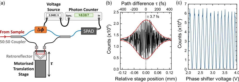
FIG. S1. Details of theg(1)(τ) measurement. (a) Schematic of the fiber Mach-Zehnder interferometer. A fiber phase shifter provides a phase shift (∆φ) to measure fringe contrast whilst a motorised translation stage controls the path difference (τ) between the two arms. The output intensity is detected by a single photon avalanche diode (SPAD) and recorded by a gated photon counter. (b) Calibration of the path difference (τ) between the interferometer arms. τ = 0 is found from Gaussian fits (red lines) to the envelope of the injected ultrafast laser pulse. (c) Example plot of fringes recorded by the photon counter as a function of ∆φby changing the voltage applied to the fiber phase shifter.
EXPERIMENTAL DETAILS
In this section we outline some additional details of the measurement setup and methods.
Interferometry - first-order correlation function g(1)(τ)
Measurement of fringe contrast
A schematic of the setup used for the first-order correlation measurements is presented in Fig. S1(a). After cross-polarised rejection of the scattered laser, the signal is passed to a fiber Mach-Zehnder interferometer, containing a fiber phase shifter (∆φ) in one arm and a motorized translation stage in the other. The intensities of the two arms are balanced with a variable fiber attenuator and their polarizations matched (typical extinction∼1000 : 1) using a pair of fiber paddles on each arm. The interferometer is placed in a thermally stable environment to minimise any phase drifts.
The stage position at which the two arms are of equal length (τ= 0) is found by injecting ultrafast pulses from a Ti:Sapphire laser emitting at the same wavelength as the QD into the interferometer, scanning the translation stage position and finding the maximum of the envelope (red lines - Gaussian fit) of the interference fringes as illustrated in Fig. S1(b). This calibration is made with the fiber phase shifter in the centre of its scan range.
To measure the fringe contrast for a givenτ, ∆φis scanned by applying a voltage sweep (step size∼0.1π, sweep rate ∼2π/3 s−1) to the fiber phase shifter. A synchronisation signal from the voltage source is passed to a gated
photon counter which records the count-rate of a single photon avalanche detector (SPAD) connected to an output port of the interferometer. An example of the trace recorded by the photon counter is shown in Fig. S1(c). We perform a generalised peak-finding routine to find the intensity at the local maximas (Imax) and minimas (Imin) of
the data and then evaluate the fringe contrast (v) according to:
v=Imax−Imin Imax+Imin
. (S26)
The maximum resolvable contrast (defined as 1−ǫ) can be checked by injecting a long coherence time single mode laser. For the interferometer used here it is limited to (1−ǫ) = 0.98 by the imperfect mode overlap of the second 50:50 fiber coupler. For low count-rates (e.g. large ∆LX), shot-noise begins to further limit the maximimum measurable
S-7
Relationship between fringe contrast andg(1)(τ)
To see how this measured fringe contrast visibility relates to the first-order correlation function of the scattered field, we consider the mode transformation that maps the scattered electric field operatorEin(t) to that detected at
the SPAD, which we labelEout(t). Neglecting retardation effects, the Mach-Zehnder described above amounts to the
transformation
Eout(t) =
1
2 Ein(t+τ∆φ) +Ein(t+τ)
, (S27)
where τ∆φ is the time delay corresponding to the phase difference ∆φ. The intensity measured at the SPAD in the
long time limit is then a function ofτ∆φ andτ, and is given by
I(∆φ, τ) = lim
t→∞hE
†
out(t)Eout(t)i=1
2g
(1)(0) +1
2Re
g(1)(τ−τ∆φ)ei(τ−τ∆φ)ωL, (S28)
where g(1)(τ) is the rotating frame steady-state first-order correlation function of the emitted field as before, c.f.
Eq. S22, and the exponential factor appears in order to convert this into a non-rotating frame measured quantity. If we now write g(1)(τ) = |g(1)(τ)|exp[iθ(τ)], whereθ(τ) is some real function capturing the phase of the correlation
function, we find
I(∆φ, τ) =1 2g
(1)(0) +1
2cos[θ(τ−τ∆φ) +τ ωL−∆φ]|g
(1)(τ
−τ∆φ)|, (S29)
where ∆φ=τ∆φωL. For fixed τ and varying ∆φ, we then see that the measured intensity has maxima and minima
given by
I(∆φ, τ) = 1 2g
(1)(0)
±12|g(1)(τ−τ∆φ)|, (S30)
which correspond to the peaks and troughs seen in Fig. S1(c).
In our measurements, the values ofImaxandIminused to find the visibility for a fixed delayτare found by varying
the phase ∆φ from approximately −15π to +15π and taking the average value of the maxima and minima. This corresponds to phase delays of approximatelyτ∆φ= ∆φ/ωL≈0.04 ps. As such the extracted values can be written
Imax= 1
2
g(1)(0) +|g(1)(τ)| and Imin =1
2
g(1)(0)− |g(1)(τ)| (S31) where the correlation function|g(1)(τ)| written above should be thought of as a time-averaged coarse grained value
with resolution∼0.1 ps. Finally, we see that the measured fringe contrast visibility is then related to the emitted field first-order correlation function through
v(τ) = (1−ǫ)|g
(1)(τ)|
g(1)(0) , (S32)
where (1−ǫ) is the maximum resolvable fringe contrast of the interferometer as discussed in the previous section. Accounting for (1−ǫ), it is thus shown that v(τ) corresponds to the absolute value of the normalised coarse grained first-order correlation function.
Spectroscopy
In Fig. 2(a) of the main text, the resonance fluorescence spectrum of the QD was presented. Here we outline the procedure used to extract the coherent and incoherent contributions for a typical spectrum. The ZPL is fitted with a Voigt profile (yellow line) which incorporates the Gaussian spectrometer instrument response. The PSB contribution (SSB(ω)) is well-approximated by a simple Gaussian function (red curve). The PSB fractionFP SB is then evaluated
from the areas (A) of these fits according to:
FP SB = AP SB
AP SB+AZP L
Performing high resolution spectroscopy of the ZPL with the Fabry-Perot interferometer (FPI) results in the inset to Fig. 2(a). As the signal is first filtered (FWHM 96µeV) by the spectrometer which is centered on the ZPL (see Fig. 1(a) of main text), the PSB contribution is removed from the high resolution measurement. Within the high-resolution spectrum of the ZPL, the broad component (blue) is the Lorentzian spectrum of the incoherent resonance fluorescence, with a linewidth governed by the transition coherence timeT2. The narrow (green) component is attributed to coherent
scattering; the linewidth observed in this measurement is limited by the Gaussian IRF (∼0.5 µeV) caused by drifts of the FPI during the measurement. We note that the natural linewidth of the incoherent peak (∼20 µeV owing to the short T2) is comparable to the free-spectral range (FSR) of the FPI; to account for this we fit the sum of a
Lorentz and a Gaussian function to the 3 peaks that occur in a scan over 3 FSRs so that the central fit accurately accounts for contributions from adjacent FSRs. After fitting, the coherent (FCS) and incoherent (FIN C) fractions of
the emission may then be calculated from the fitted areas (A) of both the low and high resolution spectra according to:
FCS= ACS
ACS+AIN C
AZP L
AP SB+AZP L
, (S34)
and:
FIN C = AIN C
ACS+AIN C
AZP L
AP SB+AZP L
, (S35)
respectively, producing the values used in Fig. 2(b) of the main text.
EXTRACTING PHONON PARAMETERS FROM EXPERIMENTAL DATA
In this section we briefly outline the fitting procedure used to characterise the electron-phonon interaction, and interpret experimental data.
Phonon dynamics in the time-domain
Now that we have expressions for the first-order correlation function, we can approach fitting the g(1) extracted
from the experimental data. Theg(1)measured at low power, shown in Fig. 1(b) of the manuscript, can be partitioned
into three separate components: below 15 ps we see a rapid decay of coherence, which we attribute to non-Markovian relaxation of the phonon environment; after this there is a slower radiative decay and ultimately a plateau at longer times, these features are attributed to incoherent and coherent scattering respectively.
To extract the phonon parameters, we therefore need only to focus on the dynamics up to 15 ps. In this situation, we can drastically simplify the expression for the correlation function, by replacing the zero-phonon line contribution with its initial value, that is the unfiltered correlation function becomesg0(1)(τ <15 ps) =G(τ)gopt(1)(τ)≈ hσ†σissG(τ).
Normalising this filtered correlation function to its value at zero time delay and restricting ourselves to positive time delays, we obtain the fitting function:
gF(1)(τ, α, νc) =
Re
∞ Z
0
˜
h(s)G(s)ds
−1 ∞
Z
0
dshh˜(s−τ)G(s) + ˜h(−s−τ)G∗(s)i. (S36)
We are now left with an expression containing two fitting parameters: the electron phonon coupling strengthα, and the cut-off frequencyνc. Through a simple root mean squared fitting, we findα= 0.0447 ps2andνc= 1.28 ps−1.
Instrument response in the weak-driving regime
S-9
-0.8 -0.4 0.0 0.4 0.8
0.0 0.2 0.4 0.6 0.8 1.0 1.2
C
o
h
e
re
n
t
fr
a
ct
io
n
Laser detuning
Polaron ME Dephasing
Dephasing + Wandering
-0.8 -0.4 0.0 0.4 0.8
Atomic Dephasing
Dephasing + Wandering
Laser detuning
-0.8 -0.4 0.0 0.4 0.8
10-4 10-3 10-2 10-1
100 Total
Coherent
P
o
w
e
r
(a
.u
.)
Laser detuning
0 10 20 30
(a)
(b)
[image:17.612.58.553.55.221.2](c) (d)
FIG. S2. Dephasing and spectral wandering for off-resonant driving: (a) Plot of the extracted detuning-dependent dephasing rateγ(∆LX). (b) Plot of the total and coherent powers calculated by the Polaron model. (c) Plot of the coherent fractionFCS
predicted by the Polaron model (solid line). The effects of including pure dephasing (γ(∆LX)) and both pure dephasing and
spectral wandering are shown by the dashed and dotted lines respectively. (d) As for (c) but for the atomic model.
We can do so in the time-domain by multiplying the detected correlation function by the instrument response functionχ(τ) = exp −τ2/∆τ2
, with temporal response ∆τ. Furthermore, we account for the finite coherence time of the laser by including an exponential decay, such that the measured first-order correlation function becomes:
g(1)m(τ) =e−τ
2
/∆τ2
e−µ|τ|g(1)opt(τ), (S37)
whereτL= 1/µis the coherence time of the laser, and we have neglected any normalisation factors.
If we assume that we are operating deep inside the weak-driving regime, such that,g(1)opt(τ)≈gcoh, we can Fourier
transformgm(1)to extract the measured zero phonon line (ZPL) spectrum, neglecting the phonon sideband contribution.
This results in a Voigt profile with a Gaussian full width at half maximum through, FWHM = 4 ln 2/∆τ. Note that we have ignored the cavity contribution here. This is because, in the regime of interest, the cavity lineshape does not vary appreciably over the frequency range of the ZPL and therefore simply leads to a constant renormalisation of the spectra. We can now fit this Voigt profile to the measured ZPL, allowing us to match the theoretical model to the experiment according to Eq. S37.
Dephasing and spectral wandering for off-resonant driving
When driving off-resonance as in Fig. 3 of the main text, we find that the polaron model tends to over-estimate the coherent fraction compared to the experiment. We note that excitation-induced dephasing due to phonons is already included within our model and thus propose that this discrepancy is due to additional pure dephasing that originates from charges generated by absorption of the laser in the doped bulk material [50]. As the behaviour for resonant driving is well-reproduced without this term (see Fig. 2 of main text), we suggest that the effect only becomes significant at larger laser detunings where the QD absorption cross-section reduces. To capture this within our model we introduce a detuning-dependent dephasing term:
γ(∆LX) =γmax(1−ξ2/(∆2LX+ξ2)), (S38)
with the linewidthξfixed as the QD natural linewidth, representing the reducing QD absorption cross-section. Fitting the Polaron model with this additional term to the experimental data gives an amplitudeγmax= 21µeV. A plot of
γ(∆LX) is shown in Fig. S2(a) whilst Figs. S2(c,d) compare the Polaron (red lines) and atomic (green lines) models
with (dashed lines) and without (solid lines) this pure dephasing term.
Compared to our experiments, the dip centered on resonance (∆2LX = 0) produced by the Polaron calculation is
somewhat too narrow. We suggest that this discrepancy arises from spectral wandering (on a timescale≫T2) in the
of tens of nanoseconds [26]. To account for these processes, we consider in Fig. S2(b) the total (Ptot - red line) and
coherent (Pcoh - blue line) powers emitted by the QD as calcualted by the Polaron model. Spectral diffusion causes
the QD to sample these functions according to the distribution of the noise. Thus, after convolving these functions with an appropriate noise distribution, the coherent fractionFCS may be evaluated according to:
FCS(∆LX) = Pcoh
(∆LX)
Ptot(∆LX)
. (S39)
As the power distributions are sharly peaked at ∆LX = 0, the convolution has little effect when driving resonantly - any
wandering results in a sharp drop in the emitted intensity and thus makes a very small contribution to the spectrum. However, away from resonance the gradient ofP with ∆LX is much smaller and the full wandering distribution is
sampled. We are thus able to extract the wandering distribution by looking at the width of the incoherent peak in a spectrum with large ∆LX such as Fig. 3(a) of the main text. Assuming a Gaussian noise distribution, fitting these
spectra with a Voigt function with Lorentzian part fixed to the QD natural linewidth allows us to extract a FWHM of 66µeV for the wandering distribution. The dotted lines in Figs. S2(c,d) show that the result of this convolution is to broaden the central dip of the calculatedFCS but with a negligible effect on the resonant case, consistent with
![FIG. 3. Phonon influences in detuned (∆LX∆atomic model, both models include additional pure dephasing and spectral wandering [39] and have upper and lower boundsfrom uncertainty in Ω](https://thumb-us.123doks.com/thumbv2/123dok_us/1793335.133889/6.612.57.561.52.222/inuences-detuned-additional-dephasing-spectral-wandering-boundsfrom-uncertainty.webp)