A Technique for the Optimization of Actuation Characteristics of Ionic Polymer-Metal Composites

Rochester Institute of Technology

RIT Scholar Works

Theses

12-2018

A Technique for the Optimization of Actuation

Characteristics of Ionic Polymer-Metal Composites

Vaughn Varma

[email protected]

Follow this and additional works at:https://scholarworks.rit.edu/theses

Recommended Citation

A Technique for the Optimization of Actuation

Characteristics of Ionic Polymer-Metal Composites

by

Vaughn Varma

THESIS

Presented to the Faculty of the Department of Mechanical Engineering

Kate Gleason College of Engineering

Rochester Institute of Technology

in Partial Fulfillment

of the Requirements

for the Degree of

Master of Science in Mechanical Engineering

A Technique for the Optimization of Actuation

Characteristics of Ionic Polymer-Metal Composites

APPROVED BY

SUPERVISING COMMITTEE:

Dr. Kathleen Lamkin-Kennard, Supervisor

Dr. Michael Schrlau

Dr. Mario Gomes

Abstract

A Technique for the Optimization of Actuation

Characteristics of Ionic Polymer-Metal Composites

Vaughn Varma, M.S.

Rochester Institute of Technology, 2018

Supervisor: Dr. Kathleen Lamkin-Kennard

Ionic-Polymer-Metal Composites (IPMCs) are a subset of Electroactive

Polymers (EAPs), which are an actively-researched class of electromechanical

actuator. IPMCs are similar in function to piezoelectric actuators, however

require substantially lower input voltage, requiring as little as 1V to

actu-ate , and with a very high maximum no-load strain of over 300%. IPMCs

can be built from biocompatible materials, and do not require the use of any

permanent magnets, making them suitable for medical applications, or for

use in environments subject to strong or fluctuating magnetic fields. IPMCs

are additionally soft and flexible, and are suitable for wet environments,

fur-ther improving their biocompatibility. This, along with their ofur-ther properties,

makes IPMCs ideal for small robotic applications and for biomimetics.

which can be provided by piezoelectric actuators or other types of EAPs. This

study expands on previous efforts to improve IPMC performance by proposing

a method for optimizing desired aspects of IPMC performance with respect to

any number of input parameters by applying the method of Gradient Descent

utilizing the Backtracking Line Search. This method is outlined generally and

demonstrated here, showing the process used through most of one iteration

to optimize for IPMC blocking force with respect to changes in the amount

of platinum used during the primary and secondary plating procedures. The

incomplete backtracking line search led to performance comparable with the

initial results (within 0.7% of this initial guess, 2.38 [mN] vs 2.37 [mN]), with

an IPMC made during the initial gradient estimation exhibiting 30%

improve-ment over this initial guess, 3.13 [mN], indicating that subsequent iterations

of the backtracking line search could lead to further improvements in IPMC

blocking force. It was additionally found that the sanding process in

partic-ular, as a process excluded wholesale from the gradient descent search used,

had a relatively large impact on the IPMC blocking force, and thus should

be controlled more carefully when continuing or extending the method carried

Table of Contents

Abstract iii

List of Tables vii

List of Figures viii

Chapter 1. Introduction and Literature Review 1

1.1 Introduction of Problem . . . 1

1.2 Literature Review . . . 4

Chapter 2. Background 16 2.1 The Gradient Descent Algorithm . . . 16

2.1.1 Gradient Estimation . . . 18

2.1.2 Selection of Sample Points for Gradient Estimation . . . 19

2.1.3 Step Size . . . 22

2.2 Testing Equipment . . . 26

2.2.1 Test Rig . . . 26

2.2.2 Data Acquisition . . . 28

Chapter 3. Methods 31 3.1 Sample Production . . . 31

3.2 Materials and Equipment . . . 35

3.3 Sensor Calibration . . . 37

3.4 Sample Testing . . . 43

3.4.1 Data Collection and Processing . . . 44

Chapter 4. Results and Discussion 49 4.1 Sample Production . . . 50

4.2 Results and Interpretation . . . 52

Chapter 5. Conclusion and Future Work 58

5.1 Conclusion . . . 58 5.2 Future Work . . . 58

Appendices 60

Appendix A. 61

Appendix B. 62

Appendix C. 63

Appendix D. 65

Appendix E. 67

List of Tables

4.1 A list of IPMC samples prepared for gradient estimation (two 1 [cm] x 3 [cm] samples for each pair of values), from Section 3.1. The first coordinate is mass of platinum salt in step 5 (initial electrode reduction step) of sample preparation, and the second coordinate is the mass of platinum salt in step 11 (secondary electrode developing process), for the full 1 [cm] x 6 [cm] sample manufactured. . . 52 4.2 Blocking forces (in [mN]) of each half of each prepared specimen 52 4.3 Blocking forces (in [mN]) of each half of the initial best guess

~

List of Figures

1.1 IPMC operating principle (from [17]) . . . 1

1.2 IPMC blocking force vs membrane thickness [9] . . . 5

1.3 Diagram showing the effects of the addition of a secondary elec-trode layer (via gold sputtering) on IPMC performance by re-ducing surface resistivity [11] . . . 12 1.4 SEM images of the nafion surface after various roughing [21] . 13

1.5 Improvements in IPMC blocking force from Orthogonal Array

Optimization [22] . . . 13

1.6 Scanning Electron Microscope (SEM) images of IPMC

elec-trode penetration resulting from different platinum concentra-tions during manufacturing [22] . . . 14 1.7 Example of the coordinate descent algorithm applied to an

el-liptical paraboloid [14] . . . 15 1.8 Examples of Gradient Descent algorithm for poorly-scaled (left)

and well-scaled (right) coordinate frames. Figures 9.14 and 9.15 from [1] . . . 15

2.1 Flowchart outlining the Gradient Descent method at a high level 17 2.2 Possible positions of points to sample for gradient estimation in

a 2D input space using n points (left) and n+1 points (right), with the best guess (?) already at the minimum cost . . . 19 2.3 Diagram showing iterations of the Gradient Descent algorithm

with too large (left) and too small (right) of a fixed step [4] . . 22 2.4 Diagram showing iterations of the Gradient Descent algorithm

with variable step sizes selected via Backtracking Line Search [4] 23 2.5 Diagram illustrating the exit condition for the Backtracking

Line Search [4]. . . 24 2.6 Fixture used for testing IPMC blocking force. . . 26 2.7 IPMC specimen set up for testing . . . 27 2.8 Diagram of force sensor used to measure IPMC blocking force [2] 28 2.9 IPMC fixture used to mount and supply power to IPMC samples

2.10 Layout of sensor showing strain gauge configuration and attach-ment to the nitinol wire. . . 30 2.11 Layout of sensor showing strain gauge positioning on the nitinol

wire. . . 30

3.1 Sensor setup during calibration . . . 38 3.2 Calibration sensor setup showing transparent box used to

pro-tect setup from drafts . . . 39 3.3 Sensor Calibration Data (incl. discarded data). Applied loads

given in grams-force ([gf]) . . . 40

3.4 Sensor Calibration Data with Linear Fit . . . 41 3.5 Dynamic sensor response to large deflection ( 2 [cm] at tip) . . 42 3.6 Undesired transient effects in sensor readings . . . 43 3.7 Normal Test Data, no visible transient effects . . . 44 3.8 Hysteresis in measured IPMC force for low input voltages . . . 45 3.9 Hysteresis observed in IPMC displacement as a function of input

voltage [8] . . . 46 3.10 Transient shift in data baseline leads to what appears to be

a large amount of hysteresis, which can be corrected by post-processing data . . . 48

4.1 Appearance of IPMC during step 5 of preparation (initial re-duction process); this differs from the description provided in [15] . . . 50 4.2 Appearance of aluminum foil lid after step 11 of IPMC

prepa-ration (secondary plating process) . . . 51 4.3 Sample Test Data, with error bars representing the 95%

Confi-dence Interval for the sensor readings . . . 57

C.1 Script used to sample sensor and drive IPMC specimen, 1/2 . 63

C.2 Script used to sample sensor and drive IPMC specimen, 2/2 . 64

C.3 Test Script Front Panel . . . 64

D.1 Early completed IPMC sample (left) and later sample (right). Boiling longer in 2N hydrochloric acid and additional sanding reduced the amount of surface area of the IPMC covered by the visible dark splotches. . . 65 D.2 Untrimmed specimen edge (left) compared against trimmed edge

Chapter 1

Introduction and Literature Review

1.1

Introduction of Problem

Figure 1.1: IPMC operating principle (from [17])

IPMCs offer advantages over many other material actuators due to

their low actuation voltage and high strains under actuation (in some cases,

beyond 90◦ deflection in a cantilever configuration)[9]. However, the range of

applications for IPMCs is still relatively limited, since the actuator force is low

to improve the maximal actuator force, and forces up to approx. 0.3 N [16]

have been observed, however the forces are still too small to find widespread

use. Furthermore, the ratio of output force to input voltage is much less than

for more widely-used actuators, such as piezoelectric actuators. Most research

into the optimization of IPMC performance to date is centered around varying

a few design variables at a time, such as actuator thickness [9] or variations in

the properties of a few chemical processes involved in IPMC manufacturing,

such as the concentration of a reducing agent [22], with only one or a few

different outputs to optimize for a given study, such as blocking force [9] or

response time [13]. Several aspects of the performance of IPMCs, such as

saturation voltage and steady-state power draw have received relatively little

attention, and could be used as metrics in classifying the utility of IPMCs as

actuators. This study seeks to build on previous research to expand knowledge

related to optimization of IPMC performance.

In order to optimize any performance metric of IPMCs, without a valid

analytical model relating that performance metric to a select set of input

pa-rameters, a technique must be used which operates totally independently of

such a model. Several of these exist and are used in practice for different

applications, such as Gradient Descent, Coordinate Descent, Genetic

Algo-rithm, and Simulated Annealing. These methods are most frequently used

in simulation, rather than in conjunction with experimentation, and are

typ-ically designed under the assumption that it takes a relatively small amount

parameters. IPMCs can, however, take several days each to make, and thus

a technique is desired which requires the preparation of a minimal number of

samples. This study seeks to utilize such an optimization technique to make it

suitable for use in optimizing IPMC performance. To that end, the following

was performed:

• Aggregated existing research on the optimization of IPMC performance

– Selected 2 process parameters to target: the concentrations of

plat-inum salt in the initial reduction and secondary developing

pro-cesses in IPMC preparation.

– Selected Gradient Descent as a suitable optimization technique to

use

– Selected blocking force as an appropriate performance metric to

optimize

• Demonstrated the chosen optimization technique as applied to improving

the selected performance metric over the parameters targeted

– Fabricated 2 IPMC samples for an initial set of values for the

tar-geted parameters

– iterated on these values according to the gradient descent technique,

using multiple samples for each set of parameter values required for

1.2

Literature Review

EAPs have potential as actuators due to their large deformation under

small input voltages and have generated sifnigifcant interest within the last ten

years [19]. During this time, new materials were developed which drastically

improved the potential for EAPs, specifically IPMCs, for practical use. There

is, however, still a substantial amount of improvement necessary to overcome

current limitations of EAPs (such as low actuation force and mechanical

en-ergy density [19]) before they can see more widespread use. Several previous

authors have explored the notion of altering various parameters related to

IPMC fabrication for better performance. Labrador [9] found, for example,

that doping the actuator in an LiCl solution drastically increased the amount

of strain exhibited under actuation. There exists a consensus among authors

who have included membrane thickness as a design variable in an

optimiza-tion study that there is inverse relaoptimiza-tionship between membrane thickness and

maximum deflection [13, 16, 19] as well as between membrane thickness and

response time [11, 16]. In addition, it is generally seen that, along with a

de-crease in maximum deflection, a thicker membrane leads to a higher maximum

actuator force [9, 11, 16]. Ruiz [19] found, however, that, at least for the case

of a rod-shaped IPMC actuator, the blocking force does not increase in an

unbounded fashion with respect to thickness; i.e. there is a finite thickness for

which the actuator force is maximum. The result was, however, derived

indi-rectly from a computational model of an IPMC and was not diindi-rectly verified

the relationship between space-charge density (which Ruiz argues is analogous

to blocking force) and specimen radius changes, if at all, with respect to other

parameters. For example, the thickness yielding maximum blocking force for

an IPMC actuator may depend on the length of the specimen. Other

re-Figure 1.2: IPMC blocking force vs membrane thickness [9]

searchers have also looked at altering different chemical properties of IPMCs

to improve actuator performance. Labrador [9] found, for instance, that

dop-ing the Nafion membrane in LiCl before manufacturdop-ing the actuator resulted

in an increase in maximum deformation of two orders of magnitude vs.

non-doped Nafion. Another approach to altering IPMC chemistry is changing the

electrode material. Researchers have used everything from Buckypaper [9] to

pure platinum [22] to palladium-platinum (Pd-Pt) [16] to gold-sputtered

spite of the fact that so many different approaches exist for fabricating IPMC

electrodes, it is difficult to directly compare the performance of different

mate-rials against one another, as there exists no controlled set of parameters under

which a wide variety of materials have been tested. Each study uses IPMCs

of a varying sizes, with varying input voltages and with inconsistent

manu-facturing processes. Along with the chemical composition of the electrodes,

different methods have been explored to improve the electrical properties of

the electrodes. In general, increasing the amount of electrode material seems

to improve actuator force without significantly affecting maximum deflection

[22]. Yu et al. [22] found that increasing the concentration of platinum during

themanufacturing stage, where an electrode is chemically grown on the Nafion

membrane, can allow the electrode to be more thoroughly embedded into the

membrane, significantly reducing the overall resistance at the interface

be-tween the electrode and the nafion membrane. The decrease in resistance was

found to lead to a significantly higher blocking force.

In general, IPMCs seem to perform better when the resistance in each

electrode is reduced, and the penetration depth of the electrode is increased.

However, researchers have yet to quantify the effects of penetration depth in

any meaningful way. One further property of the interface between the

mem-brane and electrode, which seems to be of importance along with electrode

penetration depth, is surface roughness of the ionic membrane onto which the

electrode is deposited. Some researchers have included surface roughing

but have not included any experimental justification for doing so. Wang et

al. [21] specifically observed the effectiveness of surface roughing on

actua-tor performance. Wang et al. highlighted several methods for roughing the

nafion membrane (Figure 1.2, and of these selected sandblasting, which

intro-duced an added step in IPMC manufacturing, where residual granules must

be chemically rinsed from the membrane before plating. Results from the

study demonstrated that using rougher sandblasting powder, over a longer

period of time, yields both higher maximum deflection and higher blocking

force. Plasma etching, while more costly than sandblasting, could avoid the

aforementioned complexity in manufacturing introduced during sandblasting

while potentially improving IPMC performance further. Kim et al. [7] found

that plasma etching can somewhat improve IPMC performance, however

over-treatment can reduce the actuator performance when compared against that

of an untreated specimen. Zhang et al. [23] directly compared the

effective-ness of plasma etching against sand blasting as a method for improving IPMC

performance. Zhang et al. [23] found that, while plasma etching can

out-perform sandblasting in both maximum deflection and blocking force of the

IPMC, plasma etching also greatly increases the dependence of each of those

characteristics on voltage. It is unclear, however, by the work done by Zhang

et al., how each of these treatments compares to an untreated specimen or

how the altered dependence on voltage behaves over the entire range of useful

input values (from minimum voltage for actuation to saturation voltage), as

due to the increased sensitivity of the output characteristics to changes in the

input voltage for plasma treatment. However, if this sensitivity drops off as

the voltage approaches the saturation voltage, and plasma etching can provide

consistently superior actuator performance for a range of input voltages, then

it can still be considered a viable option for improving IPMC performance, for

cases in which the input voltage can be held near or within that range during

operation.

There has been relatively little research performed to date into the

ef-ficacy of using existing optimization methods to optimize various metrics of

IPMC performance. Lacking an accurate analytical representation of these

metrics as a function of process parameters used when manufacturing the

IPMCs, optimization techniques designed for black-box testing are an

attrac-tive option, as they explicitly operate without this prior knowledge. Yu et al.

[22] sought to improve IPMC performance using Orthogonal Array Testing, a

technique traditionally used for fault testing in software [18]. This technique,

for a set of discrete inputs, seeks to find the set of inputs which leads to some

particular output (i.e. the presence of some fault) without needing to test every

single combination of inputs. The technique requires selection of orthogonal

combinations of inputs, that is inputs that are both balanced and that are

dis-similar from one another. To improve IPMC performance, Yu et al. [22] used

a set of three possible values for each of three process parameters. Low, center

and high values used were used for the concentration of reducing agent for

dur-ing this process, and the concentration of Tetraethyl Orthosilicate (TEOS),

which was mixed into Nafion solution and then cast as such into the shape

of a sample. The technique provided large improvements in blocking force

(Figure 1.5), and provided some insight into the sensitivity of the blocking

force and displacement of IPMCs subject to changes in these parameters, with

the platinum salt concentration (Figure 1.2) and TEOS concentration having

a substantially larger impact than reducing agent concentration on blocking

force and maximum deflection. However, the approach taken by Yu et al. [22]

was limited in resolution, as the input variables must be discretized roughly

to avoid excessive testing. The technique is thus most suitable for situations

where the desired variables to test are already discrete, as techniques designed

for continuous variables can often not be applied for discrete variables. Some

examples of such variables are type of metal to plate onto IPMC, cation

el-ement, and the addition of some extra manufacturing step. However, such a

technique designed for continuous variables is desireable where the variables

are, in fact, continuous, as useful information can be gained in between

adja-cent discrete steps.

Lee et al. [10] used a simple form of such a method, and attempted to

improve the blocking force of a simulated actuator assembly constructed from

multiple IPMCs, although the technique used can also be applied to physical

IPMCs as opposed to simulated ones, and can be applied to optimize the

blocking force of a single cantilevered IPMC rather than an actuator assembly.

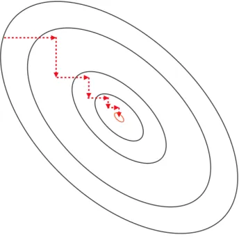
single parameter (IPMC length), given that the other parameters were all

fixed. However, this does not translate well to higher-dimensional parameter

space, as the desired output parameter may not depend on each input variable

independently of one another. Thus, if this technique were extended even to

just two parameters to vary, varying one at a time, each time a best value

is found for one parameter, another search would need to be performed with

the other parameter (Figure 1.2), until some convergence criterion is met for

both parameters. The approach could lead to a high number of iterations as

the algorithm zig-zags or spirals in on the combination of values which, when

combined, produce the best overall result (in this case, the highest blocking

force). The generalization of this technique is referred to as Coordinate Ascent,

or Descent if it is desired to minimize the output metric.

The technique of Gradient Descent described by Boyd & Vandenberghe

[1] serves as an iterative method for optimizing any quantifiable, continuous

performance metric resulting from any finite number of continuous input

pa-rameters, and avoids some of the issues arising from a more na¨ıve approach

when used for higher dimensions. The technique involves finding the gradient

of the desired output metric (cost), then iteratively performing a line search in

the direction of greatest descent and recalculating the gradient until a

conver-gence criterion is met. The approach is similar to coordinate descent/ascent,

but each line search is performed in a direction believed to give the greatest

improvement in cost.

algorithm, and highlights some of the challenges associated with the method.

If the cost is much more sensitive to changes in some directions than others,

the algorithm will have difficulty converging, and may do so very slowly. In

addition, the gradient descent method is a convex optimization technique.

Thus, it is only guaranteed to find the true minimum of the cost if the cost

is a convex manifold over the set of input parameters, ensuring that any local

minimum is also a global minimum. Otherwise, the technique may converge to

a local minimum which is not the true global minimum, providing improvement

Figure 1.4: SEM images of the nafion surface after various roughing [21]

Figure 1.7: Example of the coordinate descent algorithm applied to an ellipti-cal paraboloid [14]

Chapter 2

Background

In order to improve some quantified attribute (e.g. financial cost,

effi-ciency, impact toughness) of a process, device or system lacking a closed-form

solution by varying some controllable parameter or set thereof, numerical

tech-niques are often utilized. The most common approaches are variants of the

Gradient Descent Algorithm, which is used to iteratively drive some arbitrary

cost toward a local minimum with respect to any number of continuous input

variables. Because of the generality of this method, it is investigated here in

further depth. In addition, because any numerical technique as applied here

depends on precision in recorded measurements, a test setup is required which

is sensitive to incremental differences in loads of the scale of those supplied by

IPMCs (e.g. sufficient to differentiate between samples with 1 [mN] and 1.2

[mN] blocking force); such a test rig is described here based on [2].

2.1

The Gradient Descent Algorithm

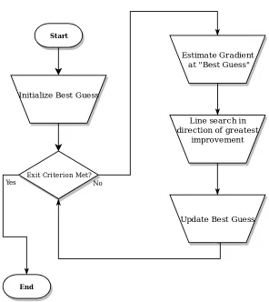
The general outline for the gradient descent algorithm is as follows:

1. Decide on a numerical calculation to minimize (for applications where

Figure 2.1: Flowchart outlining the Gradient Descent method at a high level

generator, simply take the negative of the calculation to minimize)

2. Begin with some ”best guess”, i.e. estimate of the optimal input

param-eters (i.e. the set of input paramparam-eters estimated to produce an optimal

cost)

3. Estimate the gradient of the cost with respect to the input parameters,

4. Move the best guess some amount in the direction of the steepest descent

of the gradient

5. Repeat steps 3-4 until some convergence criterion is met, or some

maxi-mum number of iterations is reached

2.1.1 Gradient Estimation

Step 3 of the above process is performed in several ways, depending on

the application and specific implementation of the gradient descent algorithm.

Here, the gradient is approximated by predictably sampling points near the

best guess and summing the vectors representing the shifts in input parameters

between the best guess and each sample. The vector is then normalized and

weighted by the improvement in the cost as follows:

~

∇C|~xi ≈

1

n

n X

j=1

_(C(~x∗

j)−C(~xi))∗(~x∗j −~xi)

||~x∗_j −~xi||

(2.1)

where C is the cost function,~xi is a vector of parameter values for theith best

guess, and ~x∗_j is the vector of parameters for the jth sampled point near ~xi.

To calculate the euclidian norm||~x∗_j−~xi||, there must be equivalence of units

across every parameter in~xi. For applications where the units do not naturally

equate, some equivalence factor must be used. For example, if one parameter

is temperature, and a second is concentration of a chemical, it could be decided

that a change of 1 mmol is ’equivalent’ to a change of 0.3 ◦C. Ideally, these

should be selected such that a change of one “unit” in any direction from the

irrespective of which variable or variables are changed.

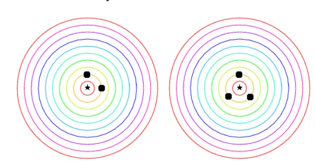
2.1.2 Selection of Sample Points for Gradient Estimation

Figure 2.2: Possible positions of points to sample for gradient estimation in a 2D input space using n points (left) and n+1 points (right), with the best guess (?) already at the minimum cost

For cases where sampling a single point is time-consuming, such as in

the production of IPMC samples, which takes multiple days, it is desirable

to sample as few points as possible while still ensuring that there exists

suffi-cient information at each iteration for the gradient descent algorithm. Na¨ıve

thinking would indicate that n points in n-dimensional space (i.e. for varying

n different parameters to improve cost) should suffice, where each point lies

along an axis aligned with the input parameters, but in the numerical case,

this may be insufficient, and may prevent the gradient descent algorithm from

converging properly. To illustrate this for a simple case, if a current best guess

truly lies on a local minimum of a smooth cost function in 2 input dimensions

de-scribed would indicate that the cost decreases most steeply in the direction

(-x, -y), when, in fact, the gradient should be approximately 0 (indicating

convergence). Thus, it is necessary that the points selected be roughly evenly

spaced about the best guess. However, if only 2 points are selected for 2 input

variables, and they are spaced evenly around the best guess, they will be

di-rectly opposite one another, and will provide no information in the transverse

direction. This can be avoided by adding a single point to sample. As a result,

for n input variables, at least n+1 points must be sampled to have sufficient

information to allow the gradient descent algorithm to function properly. The

problem of placing a minimum number of points about the current best-guess

thus becomes the problem of placing n+1 points evenly on an n-dimensional

hypersphere. A convenient method for doing this follows without proof:

1. Select one point a distance of one unit along the first input parameter

(~x∗₁ = [1 0 · · · 0]T₎

2. Assign a value of −1

n−1 for the first index of every remaining point (this

ensures that the arithmetic mean of the set of n vectors is the zero vector)

3. For the second point, assign the second coordinate a value such that the

magnitude of the vector is 1, and all values after the second coordinate

are 0 (for the 4D case, where ~x∗₁ = [1 0 0 0]T, ~x∗₂ = [−₄1

√

15 4 0 0]

T_.

4. For the remaining n-1 points, select the second coordinate as a uniform

value such that the arithmetic mean across the second coordinate is 0

5. Continue this process for all remaining coordinates and vectors. For

the last two vectors, there should be two possible values for the final

coordinate such that it has a magnitude of 1 (a positive and a negative);

these are the values for the last coordinate of each of the last two vectors.

For the 4D case, the vectors are thus:

    1 0 0 0     ,     −1 4 √ 15 4 0 0     ,       −1 4

−q5 48 q 5 6 0       ,        −1 4

−q5 48

−q5 24 q 5 8        ,        −1 4

−q5 48

−q5 24

−q5 8        (2.2)

6. Using the previously set equivalence factors, convert each value of each

vector into a corresponding input parameter with units

7. This set of vectors represents perturbations from the best guess. The

entire set may be scaled by a constant factor to ensure the following:

• That the changes in input values are large enough they produce

a measurable change (i.e. large enough with respect to all noise

resulting from process and measurement uncertainty) in the overall

cost, and

• That the perturbations are not so large as to skip over important

features of the cost over the input space (e.g. local extrema).

Gen-erally speaking, the smaller the perturbations, the closer the

ap-proximation is expected to be to the true gradient, but also the

8. Add to the set of vectors the current best guess, and these are the points

to sample at each iteration.

The perturbation vectors do not depend on the current best guess, so these

can be precomputed once and used for every iteration, meaning only the last

step is necessary to perform at every iteration.

2.1.3 Step Size

Figure 2.3: Diagram showing iterations of the Gradient Descent algorithm with too large (left) and too small (right) of a fixed step [4]

Once the estimate of the gradient has been calculated, the best guess

must be moved in the direction of steepest descend (opposite the gradient

vector) by some amount. There are several methods for determining the step

size to use, such as simply using a fixed scalar multiplied onto the magnitude of

the gradient (Figure 2.1.3), but using a fixed step size requires precise tuning

Figure 2.4: Diagram showing iterations of the Gradient Descent algorithm with variable step sizes selected via Backtracking Line Search [4]

There exist, however, methods which choose a step size adaptively, and one

such method is used here, namely the Backtracking Line Search as described

by Boyd & Vandenberghe [1]. This method is more robust than a fixed step

size to deviations in the scale of the gradient, is relatively simple, and tends

to select an appropriate step size without too many iterations (Figure 2.1.3).

The Backtracking Line Search is carried out as follows:

• Select parameters 0 < α <0.5 and 0< β < 1

– α is related to the exit condition for the backtracking line search,

and is recommended by Boyd & Vandenberghe [1] to be selected

between 0.01 and 0.3 (0.1 used here)

– β relates to how quickly the step size decreases (values closer to

1 decrease more slowly). Boyd & Vandenberghe [1] recommend

respectively. A slightly more crude search (0.4) is to be used here for

the initial line search, to balance the number of iterations required

for the line search with the desire to take a suitably large step, which

can reduce the number of times the gradient must be estimated, and

thus reduce the number of samples required overall.

• begin with a parameter t =t0, and do the following:

1. If the exit condition

C(~xi−t ~∇C(~xi))≤C(~xi)−αt∗ ||∇C~ (~xi)||2 (2.3)

is satisfied (Figure 2.1.3), exit the search with the new best guess

as~xi−t ~∇C(~xi)

2. Otherwise, updatet :=βt (this requires the production of an

addi-tional sample) and repeat.

Figure 2.1.3 provides a visualization of the Backtracking exit condition. The

slope of the lower dashed line is the gradient of the cost at t=0, f(x) is the cost

along the direction of the gradient, and the upper dashed line is the threshold

for the line search. t is updated until the sampled pointf(x+t∆x) lies below

the upper dashed line.

The entire gradient search is carried out until some exit criterion is

reached. There are a few commonly used ways to formulate this exit condition,

such as a threshold on the proportion of improvement of cost between one

iteration and the next, i.e. ∆_CC ≤ , where is a cutoff threshold, such as

= 10−4. Another common condition is that the gradient have a sufficiently small magnitude, e.g. ∇~_CC < ). These two exit criteria are similar for the

gradient descent method, as the step size at any iteration is proportional to

the magnitude of the gradient. The exit criterion ∆_CC ≤ may cause the algorithm used here to exit earlier than desired for a given , in particular if

the β selected for the backtracking search is small and α is large, as this can

cause the line search to take a step which is especially small proportional to

the gradient when compared with other steps taken, causing a smooth cost

function to have very similar values between iterations of the gradient descent

search, leading to undesired termination. The gradient descent search is not

carried out for multiple iterations in this study, and thus the selection of an

2.2

Testing Equipment

2.2.1 Test Rig

Figure 2.6: Fixture used for testing IPMC blocking force.

For testing the blocking force of the IPMC samples produced, a test rig,

shown in Figure 2.2.1 and slightly modified from that described by Chiu [2],

Figure 2.7: IPMC specimen set up for testing

opposing strain gauges affixed to the wired with JB Weld (Figures 2.2.1,2.2.1)

as a voltage divider to measure bend in the wire, and thereby applied force

at the tip of the wire. The IPMC specimen was screwed between two pads

made of 1/8” graphite gasket, each of which is connected to a wire lead with

Nickel-based conductive glue (Figure 2.2.1). The connection was sealed with

Amazing Goop all-purpose adhesive to prevent oxidation of exposed copper

Figure 2.8: Diagram of force sensor used to measure IPMC blocking force [2]

during testing, as seen in 2.2.1, along with the tip of the nitinol wire, which

was set at a distance of 1.065 [in] from the top of the graphite pads for all

tests performed. The nitinol was angled such that an IPMC sample would not

easily lose contact with the wire during testing. In order to allow the bottom

of the assembly to be submerged while mimimizing the amount of exposed

metal kept underwater to reduce rust formation, and to fit the bottom part

of the test rig into the available glassware, a new bracket (Appendix A) was

designed and 3D printed to replace the lower aluminum bracket in [2] holding

the IPMC sample.

2.2.2 Data Acquisition

An NI MyDAQ with a 10-bit Analog-Digital Converter (ADC) was

used to capture data. Both the signal pin as well as the voltage source for

the voltage divider were measured, and the sensor signal was taken to be the

signal pin voltage divided by the source voltage at every time step. The process

was done to keep the signal constant with respect to variations in the input

Figure 2.9: IPMC fixture used to mount and supply power to IPMC samples during testing

although due to the MyDAQs relatively low current limit on the analog output

pins, an op-amp circuit with unit gain was used as a buffer (Appendix B), so

that the current could be supplied by a secondary power supply rather than

the MyDAQ. Fairly severe current-limiting was still observed for higher input

voltages and for certain IPMC samples, and so the second channel of the op

amp integrated circuit (IC), as well as both channels of six additional identical

LM2094N op amps, also with a unit gain, and the outputs were connected to

Figure 2.10: Layout of sensor showing strain gauge configuration and attach-ment to the nitinol wire.

Chapter 3

Methods

3.1

Sample Production

In order to execute the gradient descent search, several IPMC samples

must be prepared and measured. For this study, IPMC samples of size 6cm x

1cm x - were made using a tweaked version of the IPMC cookbook provided by

NASA JPL [16], outlined Below. All values are presented per [cm2_{] of sample}

area and all values were multiplied by 6 [cm2_{] for the samples used here. The}

approach used was to:

1. Sand and cut IPMC sample to size from Nafion sheet. Each sample

was sanded lightly with 150 grit sandpaper, then vigorously with 800

grit sandpaper until the IPMC took on a matte, minimally translucent

appearance. In future studies, this should be replaced, ideally, with a

process which can be more precisely controlled, such as sandblasting.

Oguro [15] recommends fine glass beads in a dry sandblasting process

for 1 [s] per [cm2] of area of the IPMC sample.

2. The sample was cleaned in DI water in an ultrasonic cleaner for 1-3

3. The sample is set in boiling 2M HCl for 30 minutes

4. The sample is rinsed in DI water, then set in boiling DI water for 30

minutes.

5. The sample is immersed in Pt solution comprised of ≥3[_cmmg2] Platinum

salt in 2[_cmmL2] DI water

6. After immersing in Pt solution, ₆₀1[_cmmL2] 10% Ammonium Hydroxide

so-lution is added to balance the soso-lution’s pH. This soso-lution is left to sit

overnight.

7. Sample is placed in 6 [_cmmL2] stirring water at 40

◦_C

8. Every 30 minutes, 7 times, ₁₅1 [_cmmL2] 5% Sodium Borohdyride is added to

the stirring water, gradually increasing the temperature to 60◦C at the

end of the 7th 30-minute period.

9. 2₃[_cmmL2] Sodium Borohydride is added to the stirring water 30 minutes

after the 7th addition in step 8, and the solution is left to stir at 60◦C

for 90 minutes.

10. The sample is rinsed in DI water and immersed in 0.1M HCl for 1

hour. After this, the specimen was rinsed and allowed to sit in DI water

overnight. This step may be skipped, but was included here to allow the

11. The sample is immersed in a stirring solution comprising 4[_cmmg2] Pt salt,

8[_cmmL2] DI water, and

1 12[

mL

cm2] 10% Ammonium Hydroxide, at 40

◦_C.

12. Every 30 minutes, 8 times, 1₅[_cmmL2] 5% Hydroxylamine Hydrochloride and

1 10[

mL

cm2] 20% Hydrazine Hydrate were each added to the stirring solution,

while gradually increasing the temperature to 60◦C. At the end of the

8th 30-minute period, some of the stirring solution was sampled along

with some sodium borohydride. The solution was brought to a boil in

a water bath. If black flecks formed, the temperature of the stirring

solution was maintained at 60◦C, and more hydroxylamine

hydrochlo-ride and hydrazine hydrate were added. Periodic sampling was done

to test for the formation of black flecks. Additional hydroxylamine

hy-drochloride and hydrazine hydrate were added until said flecks no longer

formed.

13. The sample was rinsed in DI water and boiled in 0.1M HCl for 30 minutes

14. The sample was allowed to soak in 1.5M LiCl solution at room

temper-ature for 3 days.

15. The edges of the sample were trimmed by hand with a sharp knife to

remove platinum from the edges of the sample. Trimming prevented

current from routing around the Nafion due to the voltage difference

between the faces of the IPMC. Instead, it is sent through the Nafion,

inducing mechanical action. The amount of deflection was visibly much

performing this so it was been performed for each subsequent sample.

The exact effects thereof are not quantified here. The amount trimmed

off was as little as possible while ensuring that no more platinum on

the edges of the IPMC was visible (Appendix D). Ideally, this should

be performed in some more precise way than by hand with a knife,

but trimmings of width 0.008 [in] were achieved in this manner. For

the purposes of this study, to reduce the number of separate sample

preparation procedures, each sample was additionally cut in half (to

make two 1 [cm] x 3 [cm] samples), and each half was tested separately.

The cost function was selected as the negative of the IPMC blocking force,

thus maximizing the blocking force. Steps 5 and 11 were selected to vary

for the Gradient Descent algorithm, varying the mass of platinum salt during

each step while keeping the volume of water fixed. It was desired that sanding

also be included as a varying parameter, however due to the unavailability

of a suitable sandblaster, this became a difficult parameter to appropriately

quantify and vary precisely, and was thus excluded from the graident descent

search. Because the two parameters to be varied have identical units, the

conversion factors comparing the units of each parameter to one another is

unnecessary. One could be used if it was predicted that the cost would be

much more sensitive to changes in one step as compared with the other, but

lacking that insight here, this was omitted. Points were sampled at a radius of

2 [mg] from the current best guess, with an ”equivalency factor” of the same

allows that||~x∗_j−~xi||= 1 for all j. The coordinates were ordered with the steps

chronologically. Thus, using the method outlined in 2.1.1, the perturbation

vectors are as follows:

~ δx∗₁ =

2 0

[mg], ~δx∗₂ =

−1

√

3

[mg], ~δx∗₃ =

−1

−√3

[mg] (3.1)

Selecting the initial best guess as 25 mg Pt for both parameters (for an IPMC

with area 6 [cm2_{]), the points to sample for the gradient approximation are}

thus:

~x∗₁ =

27 25

[mg], ~x∗₂ =

24 26.73

[mg], ~x∗₃ =

24 23.27

[mg] (3.2)

IPMC samples were prepared for each of the above, as well as the best guess

itself.

3.2

Materials and Equipment

The materials used to create the IPMC samples as per Section 3.1 are

as follows:

• 2N Hydrochloric Acid (HCl)

• 0.1N HCl

• Nafion 117 from DuPont

• Platinum Salt (Tetraammineplatinum(II) chloride hydrate)

• Hydrazine Hydrate 20%

• Sodium Borohydride 5%

• Deionized (DI) water

• Ammonium hydroxide 10%

The equipment used during the manufacturing of IPMC samples is as follows:

• Digital Scale

• Fisher Scientific IsoTemp hot plate/stirrer with closed-loop control

(tem-perature input with resolution 5◦C)

• Thermo Scientifict Chermical fume hood

• Small pocket knife

• Branson 2510 ultrasonic cleaner

• 800 grit sandpaper

• 150 grit sandpaper

• assorted beakers and test tubes

• Eppendorf 1000 µL pipette and tips

• Aluminum foil

The materials and equipment used in testing the manufactured samples is as

follows:

• 7x LM2904N dual-channel digital op-amp

• 4x 10kΩ resistors, 5% tolerance

• Omega TrueRMS SuperMeter multimeter

• MPJA 14601PS DC power supply

• Shenzhen Mastech HY3003-3 dual-channel DC power supply

• Weller General-Duty Soldering Iron

• Assorted header pins and wires

• National Instruments MyDAQ module with LabView 2014

3.3

Sensor Calibration

To calibrate the sensor, it was removed from the test rig and clamped

to a table as shown in Figure 3.1. In Figure 3.1, a loop string was affixed to

the end of the nitinol wire with a small dab of glue. Weights of various masses

(0.05 [g] to 1.2 [g]) were cut from scrap wire to hang on this loop, and were

massed via a digital scale. While the sensor data was being collected, the setup

was covered with a plastic box jutting over the edge of the table, as shown in

Figure 3.2, to prevent drafts in the room from impacting sensor readings. A

Figure 3.1: Sensor setup during calibration

supply voltage pins at 1 [kHz] for 10 [s]. The script displayed a graph of the

set of measurements (as Vs Vi, i.e.

Vsignal

Vsupply) for visual verification, and reported the

arithmetic mean of the sensor signals. All loads were measured as the ratio of

these signals, during calibration as well as data acquisition. This helps prevent

noise in the input voltage as well as changes from touching the power supply’s

voltage knobs from impacting the sensor reading.

The sensor was measured with various combinations of weights hanging

from it, beginning and ending with none, and the results were collected in an

Excel spreadsheet. It was found that the sensor did not initially produce

meaningful results. As shown in Figure 3.3, there is a cluster of relatively

unorderd data points with no clear trend. This occured during initial loading

and unloading of the sensor and tended to drive the sensor readings toward

Figure 3.2: Calibration sensor setup showing transparent box used to protect setup from drafts

sensor, and the data taken before the readings settled to a consistent no-load

value were discarded. Because the order in which the data were collected was

preserved, and the slippage occurred only near the beginning of the calibration

procedure, the rejected data were selected as those data having been recorded

on or before the last clear outlier, as determined visually. A linear regression

was performed on the remaining data (Figure 3.4), and the slope was used

Figure 3.3: Sensor Calibration Data (incl. discarded data). Applied loads given in grams-force ([gf])

from [gf] and the slope of the curve was found to be 54.4 [N]. The sensor was

only calibrated in one direction, as all samples can be set up to press into

the nitinol wire from the same direction. Testing in a single direction is also

performed to prevent the sensor from continuing to slip after settling initially.

It was noted that, if the nitinol whisker was deflected too much (≥ 2

[cm] at the tip) during setup or during manual adjustment of the IPMC setup,

the zero-weight reading may change significantly and unpredictably. Upon

further investigation, this appears to have nonnegligible dynamic behavior

(Figure 3.5). It is believed that this is due to the nitinol wire slipping against

Figure 3.4: Sensor Calibration Data with Linear Fit

bend in the nitinol wire. Ideally, the nitinol wire should be clamped in such

a way that it cannot slip (e.g. by epoxy). In this study, to allow the nitinol

wire to be removed or adjusted if necessary, the sensor was left with just set

screws fixing the nitinol wire in place. To prevent the slippage from altering

data, the weights were added and removed carefully, and the sensor was tested

with no weights both before and after all other sensor readings to ensure this

value had not changed during testing. During testing of the IPMCs, this

dynamic sensor behavior was avoided in a similar way, by not disturbing the

sensor during testing, and by testing loading conditions in the increasing and

Figure 3.5: Dynamic sensor response to large deflection ( 2 [cm] at tip)

slippage from altering test readings, the test procedure was performed without

recording data, until the LabView display showed no signs of transient effects

in the sensor readings outside of those expected, i.e. when the data look

like Figure 3.7 as opposed to Figure 3.6. Later, post processing of the data

was performed to correct for this slipping (Section 3.4.1) thereby reducing the

number of tests necessary to gather the required data. The apparent square

wave in the data is an expected feature, and is explained in detail in the

Figure 3.6: Undesired transient effects in sensor readings

3.4

Sample Testing

A LabView script was developed to automate the test process

(Ap-pendix C). The script applies voltage in 0.1 [V] increments to the IPMC, up

to 3.3 [V], then back down to 0 [V]. Above some voltage ( 2.5 [V] for most

samples tested), oxidation began at the interface between the graphite pads

and the IPMC sample and, as some current is diverted to the oxidation

pro-cess, and lacking a way to accurately measure the voltage drop through the

graphite pads and through the interface with the IPMCs resulting from this,

test data was truncated such that data from input voltages exceeding this

Figure 3.7: Normal Test Data, no visible transient effects

3.4.1 Data Collection and Processing

Each data point was taken as the arithmetic mean of the data beginning

at some offset from the time when the voltage was first applied, to allow the

dynamics of the IPMC/sensor combination to settle to approximately

steady-state condition, and the time when the input voltage shifts again. A good

value for the offset was determined empirically, for the IPMC samples tested

here, to be 15 [s]. A smaller value may be sufficient, but this left 45 [s] of

data at a sampling rate of 1000 [Hz] for each data point, which is a substantial

amount of data, and which leaves acceptably small error bars as discussed in

Section 4.3.

Figure 3.8: Hysteresis in measured IPMC force for low input voltages

[V] to 3 [V] and back, the force did not return to its original value. However,

unlike during the sensor calibration, the deflections of the tip of the nitinol

remained well under 1 [cm] during testing, and this amount was consistent

between tests. It was discovered that creating a short circuit across the IPMC

leads, only after removing any applied voltage, caused dynamic behavior in

the IPMC (the opposite direction as when applying the voltage initially,

indi-cating relaxation in the specimen), even if the IPMC had been provided with

a 0 [V] difference between its faces prior to shorting the actuator. A similar

phenomenon was observed by Kim & Kim [8], that IPMCs retain some

dis-placement, and thus, due to the electromechanical action involved in IPMC

displacement, some voltage, even after the IPMC is supplied with a 0V

Figure 3.9: Hysteresis observed in IPMC displacement as a function of input voltage [8]

during the automated testing by applying a -3 [V] signal to the IPMC in

between each 0.1 [V] increment/decrement. This was not predicted to have

precisely the same effect as short circuiting, however it ensured that every test

was performed in the “voltage increasing” direction, and could thus be

com-pared against one another. With these changes, the overall testing procedure

for a single prepared IPMC specimen was as follows:

1. Mount the IPMC specimen in the designated fixture (Figure 2.2.1) by

screwing the graphite pads together with the IPMC in contact with the

last 1 [mm] of the nitinol wire

2. Ensure all electrical connections are wired properly, with no visible short

circuits and with all connections attached

3. Turn on power supplies (≥ 5 [V] for the Op Amp array input power, 5

4. Run test procedure in LabView

• Step from an input voltage Vipmc of 0 [V] up to 3.3 [V] in 0.1 [V]

increments, holding at each value for 60 [s] (to allow setup to

ap-proach steady-state) and with -3 [V] applied for 30 [s] before each 60

[s] interval (to ensure all measurements are in increasing direction)

• Decrement the applied voltage by 0.1 [V] from 3.3 [V] down to 0

[V], still with the 30 [s] sections of -3 [V] before ecah 60 [s] section

After applying the -3 [V] signal, however, large abnormalities in the

data persisted. It was found that the sensor data was still occasionally slipping

(Figure 3.4.1) by enough to clearly disrupt the blocking force data. To correct

for this, the difference between each recorded data point and the sensor value

associated with the previous -3 [V] section was taken, and the values were

subsequently shifted by a constant value such that the arithmetic mean of the

first and last data points (each at an input voltage of 0 [V]) lies at 0 [N] applied

force. The processing made the final data robust to shifts in the sensor data

occurring outside of regions of data used to produce each data point. The

correction does not ensure that all sources of inaccuracy of recorded data are

removed, but regularized the final data substantially, and allowed for a more

reasonable comparison between IPMC specimens. All of the processing on the

Chapter 4

Results and Discussion

In order to reduce the effect of random uncertainty in the preparation

process on the final results, it is desired to have multiple samples to compare

against one another. However, due to the time taken to manufacture a sample,

it can be difficult to produce these samples in a timely fashion. As a

com-promise, a single sample was prepared and split in two, leaving two samples

to measure for each set of variables while still only requiring a single

manu-facturing process for each pair. Overall, an initial guess was prepared, as well

as 3 pairs of nearby samples to calculate the gradient, and a single pair of

samples for the first iteration of the backtracking line search. Some differences

in appearance during the sample preparation process were observed from the

expectation outlined in [15], such as the earlier-than-expected formation of

a dull metallic layer in every sample produced; additionally, the samples cut

from the same IPMC sometimes varied significantly in blocking force, in spite

of the uniformity of the processes affecting each half of the original IPMC.

The execution of the gradient descent algorithm was carried out mostly as

expected, with the caveat that it was not anticipated that an increase in

plat-inum salt concentration should lead to much of a decrease in blocking force

data collected.

4.1

Sample Production

Figure 4.1: Appearance of IPMC during step 5 of preparation (initial reduction process); this differs from the description provided in [15]

When preparing IPMC samples, it was expected that the initial

reduc-tion process would leave a black layer of platinum particles as described in

Step 3 of [15], and a metallic sheen was not expected until the secondary

plat-ing process (step 4 of [15], step 11 in Section 3.1), however it was frequently

observed that the IPMC took on a metallic sheen before finishing with the

initial reduction process. Figure 4.1 shows this, with the gray portion on the

right overtaking the black portion on the left over the course of the reduction

in [15], but additionally, during the preparation of the first few samples, it

was found that inadequate sanding caused this process to occur more quickly,

indicating that some more effective way of sanding to increase the effective

surface area of the IPMC (e.g. sandblasting) could cause a closer correlation

with the results of [15].

Figure 4.2: Appearance of aluminum foil lid after step 11 of IPMC preparation (secondary plating process)

For the longer processes during sample preparation, aluminum foil was

used to fashion coverings for the glassware used to limit evaporation of the

solution, which otherwise sits uncovered, on heat (up to 60◦C), for several

hours at a time. It was noted that after the secondary platinum developing

process, the aluminum foil changed in apperance, developing a thin black layer

on the surface exposed to the evaporated vapors of the stirring solution (Figure

4.1), which condensed on the aluminum foil. It is possible that this black layer

the weak reducing agent, which condensed onto the aluminum foil. This might

indicate that a nonmetallic cover should be used, to ensure that the IPMC is

the only surface onto which the platinum in solution will develop, however

since an aluminum cover was used during initial sample preparation, one was

used for every sample made, to ensure comparability between all prepared

samples.

4.2

Results and Interpretation

~x1 ~x∗1 ~x∗2 ~x∗3

25 25 27 25 24 26.7

24 23.3

Table 4.1: A list of IPMC samples prepared for gradient estimation (two 1 [cm] x 3 [cm] samples for each pair of values), from Section 3.1. The first coordinate is mass of platinum salt in step 5 (initial electrode reduction step) of sample preparation, and the second coordinate is the mass of platinum salt in step 11 (secondary electrode developing process), for the full 1 [cm] x 6 [cm] sample manufactured.

Fblock

~

x1 ~x∗1 ~x

∗

2 ~x

∗

3

2.26 3.41 1.35 1.18

2.48 2.84 0.94 0.53

Table 4.2: Blocking forces (in [mN]) of each half of each prepared specimen

After the data was processed as outlined in Section 3.4.1, the values

at each voltage increment in the increasing and decreasing directions were

3 cm x 1 cm specimen prepared. The average of these values was used to

calculate the gradient as follows:

~

∇F|~x=~x1 ≈

1 3 3 X j=1

(F(~x∗_j)−F(~x1))∗δ~x∗j

=

0.708 0.0829

[mN] =

1.42 0.166

N g

(4.1)

whereδ~x∗_j is unit-normalized using the conversion factors described in Section

2.1.1, giving it a magnitude of 1 [-] for all j. This result indicates that, for the

IPMC preparation process described in Section 3.1 for 1 [cm] x 6 [cm] samples,

using 25 [mg] of Pt each for steps 5 and 11, the blocking force is much more

sensitive to the addition of platinum in the initial reduction process (step 5)

than in step 11. This could be related to the formation of a metallic sheen in

the initial reduction phase, and, if it is the case that the sensitivity of blocking

force to changes in platinum concentration in the secondary plating process

is itself dependent on the amount of sanding the IPMC receives, this only

serves to further demonstrate the need for an optimization technique which

can account for multiple interdependent factors, such as the gradient descent

method used here.

Since the Cost C(x) is taken to be the negative of the blocking force

for the gradient descent algorithm, the behavior of the algorithm is that of the

analogous gradient ascent with the blocking force as the objective function.

A value of t0 = 5[N−1] was selected to ensure the first sample in the

line search is sufficiently far from the initial best guess to reduce the number

Fblock

~

x1 ~x2

2.26 2.44

2.48 2.33

Table 4.3: Blocking forces (in [mN]) of each half of the initial best guess ~x1

and the first iteration of the backtracking search ~x2

check in the line search (from Equation 2.3) is

C(~x1−5∇C~ (~x1))≤C(x~1)−0.5∗ ||∇C~ (~x1)||2 (4.2)

This leaves the first point to be sampled for the line search at

x=~x1−5∇C~ (~x1)

=

25 25

[mg] + 5∗

1.42 0.166

[mg]

=

32.1 25.8

[mg]

(4.3)

One pair of 1 [cm] x 3 [cm] (one 1 [cm] x 6 [cm] Nafion strip) IPMCs were

manufactured with these amounts of platinum, and the maximum blocking

forces of each are collected in Table 4.2. The average of these (2.38 [mN]) does

not satisfy the line search termination criterion, as

C(~x2)> C(~x1)−0.5∗ ||∇C~ (~x1)||2

−2.38[mN]>−3.39[mN]

(4.4)

Although it appears that this method has led the search in a direction with

lit-tle benefit (as the blocking forces of this and for~x1 are similar to one another),

however circumstances like this are accounted for with the backtracking line

but closer to~x1 with substantially better blocking force, and the backtracking

search will walk back toward~x1 to find a suitable point. Thus, the next step

of the gradient descent algorithm is to continue with another iteration of the

backtracking line search, with t =βt0 = 2, now checking the criterion

C(~x1−2∇C~ (~x1))≤C(x~1)−0.2∗ ||∇C~ (~x1)||2 (4.5)

One interesting result of this, however, is the implication of the existance of a

local minimum between the initial guess and first iteration of the line search.

Although nothing precludes this from occurring, conventional reasoning

indi-cates that an increase in platinum salt concentration consequently increases

conductivity on the surface of the IPMC, while also affecting the IPMC

thick-ness and overall stiffthick-ness minimally, thus increasing the maximum deflection

and blocking force at the tip of the IPMC. However, barring some unexpected

perturbation to the data forcing both samples of ~x∗₁ to be recorded with an abnormally high blocking force, or ~x2 with an abnormally low blocking force

(both relative to~x1), that is what this data indicates: that by increasing the

platinum salt concenteration primarily in step 5, the IPMC samples exhibit the

expected increase in blocking force, then, somewhere, the minimum is reached

and the blocking force declines thereafter, such that by ~x2 with t=[5N−1],

the blocking force is approximately identical to that at ~x1. As can be seen

in Table 4.2, some values (esp. ~x∗₃) have a fairly large disparity in blocking force between the two samples. These samples were produced from the same

strip of Nafion, as a single unit, so it is somewhat surprising to see blocking

relatively poor control over uniformity, as it is performed here by hand and

verified visually. It is noted in [21] that the blocking force is fairly sensitive

to changes to the sanding process, and thus it would likely be advantageous

to implement this process in a more predictable, uniform fashion. This would

additionaly provide a way to include sanding in the gradient descent search,

for instance by varying grain size and time in a sandblaster; given the

sensi-tivity of the desired metric to improve, blocking force, to sanding, this could

allow for much greater improvement overall in IPMC blocking force than is

possible by only varying the concentrations of platinum as performed here.

4.3

Measurement Uncertainty

One interesting finding from the data gathered is that some of the

apparent uncertainty or noise in the blocking force values is not captured in

the sensor noise. The error bars in Figure 4.3 are small enough to indicate

that, for the amount of data averaged and the noise in that data for each input

voltage, the blocking force values indicated should be more precise than they

apparently are. None of the data points sharing an input voltage, for instance,

have overlap in their error bars, indicating that the sensor noise represented by

the shown error bars is possibly not indicative of all measurement uncertainty.

This is possibly due to a change in the contact location or angle between

the IPMC tip and the sensor whisker, as the specimen is not affixed to the

sensor, but merely rests against it. Given the sensitivity of the sensor, and

Figure 4.3: Sample Test Data, with error bars representing the 95% Confidence Interval for the sensor readings

the eye and still produce this behavior. That said, the data still do form a

relatively clear underlying curve from which information can be drawn, but

further characterization of the utilized sensor device as it interacts with IPMCs

Chapter 5

Conclusion and Future Work

5.1

Conclusion

Based on prior research, platinum salt mass in each plating process

was targeted as the set of parameters to vary, and the gradient descent

tech-nique with a backtracking line search was selected as an iterative optimization

method for improving IPMC blocking force. This process has been generally

outlined to optimize arbitrary performance metrics of IPMCs with respect

to any number of relevant, controllable input parameters, and was partially

demonstrated for the inputs of platinum salt mass and output metric of

block-ing force. This method, if carried out through several iterations, could serve to

establish precise process parameters to prepare IPMCs with optimal (locally,

at least) performance, thus improving their overall viability as actuators. This

leaves some work for future researchers to carry out in order to see the

opti-mization of IPMC actuation characteristics fully come to fruition.

5.2

Future Work

The process outlined here for optimizing IPMC performance wa