Time-dependent probability density function in cubic stochastic processes
Eun-jin KimSchool of Mathematics and Statistics, University of Sheffield, Sheffield, S3 7RH, United Kingdom
Rainer Hollerbach
Department of Applied Mathematics, University of Leeds, Leeds, LS2 9JT, United Kingdom
(Received 28 June 2016; revised manuscript received 23 August 2016; published 10 November 2016) We report time-dependent probability density functions (PDFs) for a nonlinear stochastic process with a cubic force using analytical and computational studies. Analytically, a transition probability is formulated by using a path integral and is computed by the saddle-point solution (instanton method) and a new nonlinear transformation of time. The predicted PDFp(x,t) in general involves a time integral, and useful PDFs with explicit dependence on xandt are presented in certain limits (e.g., in the short and long time limits). Numerical simulations of the Fokker-Planck equation provide exact time evolution of the PDFs and confirm analytical predictions in the limit of weak noise. In particular, we show that transient PDFs behave drastically differently from the stationary PDFs in regard to the asymmetry (skewness) and kurtosis. Specifically, while stationary PDFs are symmetric with the kurtosis smaller than 3, transient PDFs are skewed with the kurtosis larger than 3; transient PDFs are much broader than stationary PDFs. We elucidate the effect of nonlinear interaction on the strong fluctuations and intermittency in the relaxation process.
DOI:10.1103/PhysRevE.94.052118
I. INTRODUCTION
Many systems in nature or laboratories not only involve stochastic processes due to intrinsic variability, or to uncer-tainty in the system, but may also be far from equilibrium. Computing the time evolution of the probability density function (PDF) of such systems is often a major challenge. While in thermal equilibrium the same level of fluctuations can be maintained by a reservoir (e.g., heat bath) at a fixed temperature (e.g., by the fluctuation-dissipation theorem [1]), far from equilibrium such a reservoir no longer exists. The level of fluctuations in the system thus changes with time and becomes a dynamical variable itself. For instance, drastic change in fluctuations can be caused by a sudden change in the temperature at the reservoir, or just by an initial out-of-equilibrium PDF. Consequently, a full knowledge of the time evolution of PDFs becomes critical.
As a simplest model, a Gaussian process has been widely used to understand a variety of stochastic processes [2,3]. At the heart of a Gaussian process is Brownian motion (random walk) driven by white noise (random noise with a very short memory), where mean square displacement increases linearly with time while there is no change in mean displacement. When subject to a linear force, it becomes the Ornstein-Uhlenbeck (O-U) process, which is a prototypical model for a noisy relaxation system, heavily used and extended in many areas of physical science and financial mathematics (e.g., Refs. [2,3]). This model is governed by the following Langevin equation for a random variablex(say, the position):
dx
dt = − ∂V
∂x +ξ, (1)
where a linear force∂V∂x =μoxis given by a quadratic potential V(x)=μox2/2. Here μo is a non-negative constant and ξ is the white noise characterized by the following statistical
property:
ξ(t)ξ(t) =Dδ(t−t), (2) where D is a constant. The angular brackets in Eq. (2) represent the ensemble average over the noise. Given the initial condition (initial PDF), the time evolution of the PDF in the subsequent time is precisely known as the joint distribution with a Gaussian transition probability. In particular, when the initial PDF is strongly peaked atx=x0, the marginal PDF of x, call itp(x,t), has the following time evolution:
p(x,t)=
β πe
−β(x−x)2
, (3)
wherexis the mean position, andβis the inverse temperature given as
x =x0e−μot, 1
2β = (x− x)
2 = D(1−e−2μot)
2μo
, (4)
In a long time limit, a PDF approaches a stationary Gaussian distribution where the variance of the PDF is set by x2 =
D/2μo. This stationary distribution can be linked to thermody-namic equilibrium distribution by the fluctuation-dissipation theorem by using 1
2x 2 = 1
2T (with the Boltzmann constant
kB =1) and Eq. (4) ast→ ∞as follows:
T = 1
2β(t → ∞)= D 2μo
, (5)
which is the Einstein’s relation. We note that a factor of 1/2 in the last term in Eq. (4) and (5) is due to our definition of D in Eq. (2); that is, conventionally, Eq. (2) is defined with 2D instead of D. For small time, the effect of the linear force is negligible compared to dx
tractability in computing various statistical quantities (e.g., all even moments determined by second moments, etc).
Gaussian statistics, however, has serious limitations in explaining emerging complex phenomena such as anoma-lous transport (super- or sub-diffusion), intermittency, self-organisation, or phase transition where a long-range correla-tion plays a key role [4–21]. In fact, non-Gaussian PDFs often observed in these systems have stimulated active research on nonequilibrium statistics by considering nonlinear interaction, finite-correlated or Levy-flight noise, multiplicative noise, fractional calculus, etc. (e.g., see Refs. [4–15,17,19–23]). The main aim of this paper to shed light on this issue by elucidating the effect of nonlinear interaction during the relaxation process of an initial PDF to a final stationary PDF as an example of nonequilibrium processes.
To gain the key insight, it is valuable to consider the simplest nonlinear version of Eq. (1) that has the same symmetry property under x → −x as the O-U process and compare results with the O-U process [e.g., Eq. (3)]. To this end, we consider a cubic nonlinear force (∝x3) for a quartic potential V(x)=μx4/4 in Eq. (1) while keeping the same
short-correlated noiseξ given in Eq. (2). The cubic force has in fact been widely used to model enhanced diffusion in various systems, including mixing in stellar interiors (e.g., Ref. [24]) and self-organization of shear flow by generalizing a sand pile in a continuous limit [14,20,25]. In particular, Ref. [20] showed that similar stationary PDFs are obtained from a zero-dimensional dynamical model, one- and two-zero-dimensional (1D and 2D) fluid models. This suggests important implications of the results from a Langevin equation with cubic nonlinearity for a broad range of other physical problems with the same highest nonlinearity.
For the cubic process, the prediction of time-dependent PDFs has proven to be elusive [2]. However, a stationary distribution can easily be shown to be a quartic exponential PDFp(x,t)=N e−βx4whereN ∝β−1/4(see AppendixAfor its property), to which any initial PDF relaxes in the long time limit. In this paper, we report on time-dependent PDFs using analytical and computational studies. Analytically, a path integral formulation [12,14–16,21,26–33] and a nonlinear time transformation are utilized to predict a transition probability. The PDF given in the path integral is computed by the saddle-point solution (instanton method) (e.g., see Refs. [14–
16,21,27–29,31,32]). The predictedp(x,t) in general involves a time integral, and useful time-dependent PDFs with the explicit dependence onxandtare presented in certain limits (e.g., in the short and long time limits). Numerical simulations of the Fokker-Planck equation present detailed evolution of the time-dependent PDF and confirm our analytical predictions.
We note that instantons originated in quantum mechanics as a nonperturbative way of computing the transition amplitude from one ground state to another. The basic idea is that the uncertainty relationship between position and momentum allows one to formulate the transition amplitude from the initial to the final position by a path, and the transition amplitude from one ground state to another can be isolated by considering Euclidean action by taking time to be imaginary. An instanton is a saddle-point solution of Euclidean action and corresponds to one particular path that leads to the transition amplitude between ground states and was used in gauge
field theory to compute the transition amplitude from one vacuum to another [31]. About 20 years later, the method was adapted to a classical fluid problem [32] and to a plasma problem [14–16]. In particular, Refs. [27–29] reported a series of detailed calculations for (multi)-instantons for double wells and different anharmonic potentials in quantum mechanics. Refs. [14–16] utilized it to predict stationary PDF tails of anomalous transport due to large events by taking a long-time limit, while Ref. [21] generalized this methodology to predict the time-dependent PDF for the O-U process without taking such a long-time limit. It is the purpose of this paper to extend this work further to nonlinear stochastic processes. The contribution of this work lies in the prediction of the time-dependent PDFs p(x,t) by calculating the instanton solutions which satisfy the boundary conditions at the initial and final times (see Sec.II).
The remainder of the paper is as follows. We present the path integral solution of PDFs in Sec.II. Exact time-dependent PDF by simulations are provided in Sec. III. Section IV
contains discussions and conclusions.
II. ANALYTICAL PREDICTION
We consider the evolution of a random variablex under a quartic potentialV(x)=μx4/4 in Eq. (1) and a white noise given by Eq. (2) as
dx
dt = −μx
3+ξ, (6)
whereμis the frictional constant for the cubic force. To gain a key insight into the evolution of this system, it is useful to obtain the equation for the mean and fluctuating components ofx by lettingx= x +δx in Eq. (6). Herexandδx are the mean value and fluctuation so thatδx =0. Then the time evolution ofxandδxcan easily be shown to be as
dx
dt = −μ[(x
2+ (δx)2)x + (δx)3], (7)
dδx
dt = −3μx
2δx+G+ξ, (8)
where G=3x[(δx)2− (δx)2]+(δx)3− (δx)3. For
small fluctuation, we can apply the quasilinear analysis to ignoreGand(δx)3in Eqs. (7)–(8) and obtain approximate
equations:
dx
dt = −μ[x
2+ (δx)2]x, (9)
dδx
dt = −3μx
2δx+ξ ≡ −μ
oδx+ξ, (10)
where μo=3μx2 is the (linear) force constant for δx. When fluctuations are negligible compared to the mean value [(δx)2 x2], Eq. (9) becomes dx
dt = −μx3, with the solution x =x0/
√
1+2μx2
0t given the initial condition
x(t =0) =x0. As the fluctuationδx increases in time, the second term in Eq. (9) gives the enhanced force, leading to the faster movement of the PDF peak fromx0towardsx =0 (see
For analytical computation of a time-dependent PDF, we consider a narrow initial PDF approximated by theδfunction p(x,t =0)=δ(x−x0). In order to obtain a PDF at any later
time, we utilize a path integral formulation by expressing the transition probabilityp(xf,tf;x0,0) between initialx0att =0
andxf at later timet =tf [12–16,21,26,30,33] as follows:
p(xf,tf;x0,0)∝ (xf,tf)
(x0,0)
Dx[t]Dx[t]e−S, (11)
whereSis the action given by (see AppendixB)
S=
tf
t0
dt
−i
dx dt +μx
3
x+1 2Dx
2+ψ(x)
. (12)
Herex is the conjugate variable tox [e.g., see Eq. (B3) and also Eqs. (3)–(5) in Ref. [16]], which effectively captures the effect of the stochastic forcingξ.ψ= 32μx2in Eq. (12) is due to the coordinate transformation between ξ and x. As ψ is negligible in the limit of smallD[12], we drop this term for analytical tractability below. The transition probability given in Eq. (11) involves the integration along all the paths connecting initial (x0,0) and final (xf,tf) points. We evaluate Eq. (11) approximately to leading order inD by finding a particular path which makes the largest contribution to the action S. This is the so-called saddle-point solution (instantons) which minimizes the actionS, satisfying the zero variation ofSwith respect toxandxas follows:
δS
δx =0→i
dx dt +μx
3
=Dx, (13)
δS
δx =0→i
dx dt −3μx
2x
=0. (14)
Equations (13)–(14) are to be solved with the boundary conditionsx(t =0)=x0andx(t =tf)=xf. We note that the crux of the instanton method is to capture a nontrivial “time-varying state” as our basic state. As noted in the introduction, instanton solutions satisfying boundary conditions were used for the computation of the time-dependent PDFs for the O-U process [21].
The explicit appearance of the conjugate variable x in Eqs. (13)–(14) reflects a vital role of the stochastic forcing in the determination of a saddle-point solution. That is, the leading order contribution to the action cannot be obtained by simply ignoringξ in Eq. (1). Saddle-point solutionsxsandxs to Eqs. (13)–(14) then give the effective actionSeff, simplifying
Eq. (11) as follows:
p(xf,tf;x0,0)=Nexp[−Seff], (15)
where N is a normalization constant to satisfy
dxfp(xf,tf;x0,0)=1 andSeffis the effective action
Seff =
tf
0
dt 1 2D
dxs dt +μx
3
s
2
(16)
= −
tf
0
dtD 2x
2
s. (17)
In the following, in order to obtain saddle-point solutions to Eqs. (13)–(14), we introduce a nonlinear (nonlocal) timeτ as
τ(t)=
t
0
dt1[x(t1)]2, (18)
and recast Eqs. (13)–(14) in terms ofτ as follows:
1 3
d dτ[x
3e3μτ
]= −iDxe3μτ, (19)
d dτ[xe
−3μτ
]=0, (20)
by using dtd =x2dτd. See AppendixCfor an example of how the transformation (18) works. The solutions to Eqs. (19)–(20) are found as
x(t)=x(t=0)e3μτ, (21)
(x(t))3e3μτ =x03+B[e6μτ−1], (22)
where
B= −iDx(t =0)
2μ . (23)
The boundary conditionx(t =tf)=xf fixes the value ofB as
B= x
3
fe3μτf −x03
e6μτf −1 , (24)
whereτf =τ(t=tf). In terms ofx(τ),tis determined by the inverse of Eq. (18) as
t =
τ
0
dτ1
1
[x(τ1)]2, (25)
while the effective actionSeff in Eq. (17) is expressed by
Seff=
2μ2B2
D
τf
0
dτ1
e6μτ1
[x(τ1)]2, (26)
where Eqs. (21), (23), and (24) are used. In the following two subsections, we separately consider the casesx0=0 and
x0=0.
A. x0=0
Forx0 =0, the time evolution of the PDF involves only a
change in its width until it becomes the stationary exponential PDF in the long time limit. Equation (22) is simplified in this case as
[x(τ)]3 =B0(e3μτ−e−3μτ),
B0 =
x3
fe3 μτf
e6μτf −1. (27)
With the help of Eq. (27), Eq. (25) can be expressed as
tf = 1
2μB
2 3 0
zf
0
dz1
1
1−z3 1
2 3
= 1
2μB
2 3 0
sin−31 2,3
(zf). (28)
Here z1=(1−e−6μτ1)13 andzf =(1−e−6μτf)13. sin−31 2,3
Ref. [34] and Appendix D) with p= 32 and q=3, which satisfy the generalized trigonometric identity
|sinp,q(zf)|q+ |cosp,q(zf)|p =1. (29)
Equation (28) thus gives us the expression forzf in terms of timetf as
zf =sin3 2,3(2μB
2 3
0tf). (30)
On the other hand, the effective actionSeff in Eq. (26) can be put into the following form:
Seff =
μB
4 3 0
D
zf
0
dz1
1
1−z31
5 3
= μB
4 3 0
2D
⎡ ⎣2μB
2 3 0tf +
zf
1−z3
f
2 3
⎤
⎦, (31)
where we used Eq. (28) and the following identity (see AppendixE):
z
0
dz1 1−z31 −5/3
=1 2
z
0
dz1 1−z31 −2/3
+z(1−z3)−2/3
.
(32)
By using Eq. (27), we rewrite Eq. (31) as
Seff =
μ 2D
2μB02tf + x4
f
(1−e−6μτf)
. (33)
The substitution of Eq. (33) into Eq. (15) then determines how PDFs vary withxfdepending ontf. The normalization factor N =N(t) in Eq. (15) alters the overall amplitude of the PDF and is discussed in Sec.II C.
Equation (33) involves τf andB0, which is a function of
τf. Sinceτf =
tf
0 dt1[x(t1)]
2,p(x,t) is not given by a simple
function ofx andtbut as an integral.
In the short and long time limits, the PDFs can, however, be approximated by a function depending onxandt. To demon-strate this, we examine the behavior oft andSeffin Eqs. (28) and (33) in the short and long time limits, respectively. First, in the long time limit (zf →1), sin−31
2,3
(zf)→ 12π3
2,3, where
π3
2,3is the generalizedπp,q(see AppendixD). Thus, Eqs. (28)
and (33) give us to leading order in 1/tf
z3f ∼1−
π3 2,3
4μtfxf2
3
,
Seff ∼ μ 2Dx
4
f
⎡
⎣1+
π3 2,3
4μtfxf2
3⎤
⎦. (34)
Equation (34) shows how the PDF evolves into the quartic exponential PDF in a long time limit. We can estimate the time required to reach the stationary state by examining the behavior of the PDF width in Eq. (34). To do this, we let α=π3
2,3/(4μtf) and findxf forSeff =1 (i.e., the width at
half-peak):
μ 2D
xf4+α
3
xf2
=1.
Solving the above by perturbation as xf =xf(0)+x
(1)
f + · · · for smallα 1 leads us to
xf ∼
μ
2D
1 4
1−
μ
4D
3 2
π3
2,3
4μtf
3
.
The leading order solution xf(0)=(μ/2D)1/4 represents the width of the stationary PDF, which is much wider than the width∝D−1/2in the case of the linear O-U process for small
D. From the condition that the second, time-dependent, term is much smaller than the first term in the above, we obtain an estimate for the critical timetcrequired to reach the stationary state:
tf > π3
2,3
8√μD (≡tc). (35)
Interestingly, the critical time tc increases as D−1/2 as D decreases. That is, the smaller the diffusion, the longer the relaxation time tc. This should be contrasted to the linear friction case where the relaxation time is independent ofD and solely determined by the friction μ. This dependence of the relaxation time on D reveals one of the important characteristics of the nonlinear process where the diffusion sets not only the spatial structure (width), but also the time structure.
On the other hand, in a short time limit (zf →0), we eval-uate sin−31
2,3
(zf)∼zf+16z4f and useB0z3f =xf3(1−z3f)
1/2
to obtain
z6fsin−31 2,3
(zf)
3
=z6f
zf+ 1 6z
4
f
3
= 2μtfxf2
3
1−z3f. (36)
We can then find the leading order solution to Eq. (36) for small 2μt x2
f in the following form
zf3 ∼ 2μt xf2 1−μt xf2,
B02= x
6
f 1−z3f
z6
f
∼ x
6
f 1+2μtfxf2
2μtfxf2
2 ,
thereby obtaining
Seff ∼ x
2
f
2Dtf
1+3 2μtfx
2
f
. (37)
The parameter 2μt xf2 physically represents the effect of a nonlinear damping, and the limit of the small value of this parameter corresponds to considering a sufficiently small time during which the effect of nonlinear damping can be considered to be small and thus computed as a small perturbation from no damping case.
The leading order behavior Seff ∼xf2/2Dtf reveals that initially, the evolution of the PDF is governed by the Gaussian process with the Gaussian PDF. The quartic termx4
PDF in the long time limit, shown in Eq. (34). For x0=0 considered in this subsection, the relaxation of a transient PDF undergoes two stages: the first is the Gaussian evolution where the white noise causes the Brownian motion with a negligible effect of the nonlinear force. When the nonlinear force becomes sufficiently large, the PDF broadens its width, settling in to the stationary quartic exponential.
B. x0=0
Unlike the case x0=0, the time evolution of the PDF is
governed by the movement of the peak of the PDF fromx0 tox =0 as well as the broadening of the PDF. Consequently, the relaxation of a transient PDF is more complex compared with thex0=0 case considered in the previous subsection. In
the following, we show that the relaxation of a transient PDF involves one more stage between the initial Gaussian evolution and the final settling in to the quartic exponential PDF. The extra stage appears when the nonlinear force becomes sufficiently large and leads to alinearforce with the effective force coefficient 3μx2 for fluctuations. That is, the second
Gaussian evolution is approximately the O-U process with the effective linear forceμ0=3μx2, similar to the quasilinear
result in Eq. (10).
In order to obtain the PDF, we need to findSeff in Eq. (15)
via Eqs. (26), (25), and (22). To this end, it is convenient to rewrite Eq. (22) in the following form:
x3=Be3μτ+αe−3μτ =Be−3μτ[e6μτ−γ], (38)
whereBis given by Eq. (24) and
α=x03−B =x
3 0e6
μτf −x3 fe3
μτf
e6μτf −1 ,
γ = −α B =
x3 0e6
μτf −x3 fe3
μτf
x3
0−xf3e3μτf
. (39)
With no loss of generality, we takex00 in this paper since
the symmetry of our cubic system underx → −xguarantees exactly equivalent results forx0<0. Equation (39) reveals the
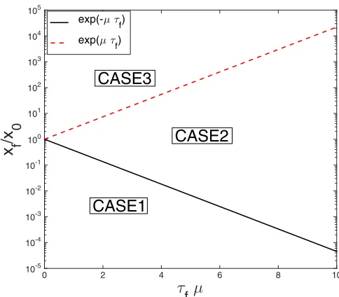
following three different cases depending on the sign ofγand the ratio ofxf tox0:
CASE1:γ > e6μτf (x
f < e−μτfx0);
CASE2:γ <0 (e−μτfx
0< xf < eμτfx0);
CASE3: 0< γ < e6μτf (x
f > eμτfx0).
Whenx0=0,γ =1, recovering the case in the previous
subsection and thus CASE2 becomes irrelevant. That is,x0=
0 leads to the appearance of CASE2. Forx0>0, a schematic diagram for the different cases is shown in Fig.1wherexf is plotted againstτf. From Fig.1, we observe that a short time behavior is described by CASE1/CASE3 while a long time behavior is obtained from CASE2. Asτf increases from zero, the region for CASE1/CASE3 gradually decreases while the region for CASE2 increases. The crossover between CASE1 and CASE2 is set byxf =x0e−μτf ≡xcwhile the crossover between CASE2 and CASE3 is set byxf =x0eμτf ≡xb. Here xc=x0e−μτf is the characteristic of the movement of the PDF
peak. Consequently, the left side of the PDF peak is described
τ
fμ
0 2 4 6 8 10
x
f/x
010-5 10-4 10-3 10-2 10-1 100 101 102 103 104 105
exp(-μ τ
f)
exp(μ τf)
CASE2
CASE3
[image:5.608.313.555.70.282.2]CASE1
FIG. 1. A schematic diagram ofxf/x0againstμτf. by CASE1 while the right side of the PDF peak by CASE2. On the other hand,xb=x0eμτfcharacterizes the boundary around
which the PDF becomes negligible asSeffbecomes very large
(details not shown here). That is,xbsets the boundary between the region of a small probability due to a stochastic noise and a dead zone. (That is, the probability is zero for xf > xb in CASE3.) To appreciate the meaning ofγ, we rewrite
γ = x
3
b −xf3 x3
c −xf3 ≡ b
,
where =xc−xf and b =xb−xf. Since and b measure the deviation ofxf fromxcandxb, respectively, the probability becomes larger for smallerand largerb. For instance, CASE1 with the large value ofγ corresponds to the region where the probability is largest.
To determine the relation between tf andτf alongxf = x0e−μτf, we note that Eq. (39) gives α=x3
0 and B =0.
Thus, the saddle-point solution in Eq. (38) is simplified as x =x0e−μτ, leading totfin Eq. (25):
tf =
τf
0
dτ1 1 [x(τ1)]2 =
1 2μx02(e
2μτf −1)
= 1 2μx2
0
x02 x2
f −1
,
and consequently
e2μτf = x
2 0
x2
f
=1+2μtfx02. (40)
In the following subsections, γ >0 (CASE1) and γ <0 (CASE2) are separately considered. (The analysis fory−γ > 0 is included in AppendixFfor completeness.)
1. CASE1:γ0(α >0, B<0), xf <x0e−μτf
γ−y >0 (sinceγ−e6μτf >0) to obtain
tf = 1
6μB23
I0, (41)
where
I0 = yf
1
dy
y23
1
(γ −y)23
, (42)
andyf =e6μτf. The integral in Eq. (42) can be written in terms of the generalized two-family inverse hyperbolic sine (e.g., see Ref. [34]). On the other hand, Eq. (26) can be shown as
Seff =
μB43
3D I1 = μ
6D
6μtf|αB| −3|B|
4 3[y
1 3(γ−y)
1 3]yf
1
, (43)
where
I1=
yf
1
dy y
1 3
(γ−y)23
. (44)
In the second line in Eq. (43), we used Eq. (41) and the identity (see AppendixG):
I1 =1 2
γ I0−3[y13(γ−y) 1 3]yf
1
. (45)
Equation (43) shows that Seff becomes zero along the char-acteristics xf =x0e−μτf as B =0. Recall that along these
characteristics, Eq. (40) holds. This means that the PDF takes its maximum value along these characteristics. To facilitate the analysis, it is thus useful to consider the deviationfrom the characteristics
=x0e−μτf −xf, (46)
where0 since xf x0e−μtf. By using Eqs. (24), (39),
and (44) in Eq. (43), we obtain
Seff =
μ 2D|B|
2μtf(x03+ |B|)− xfe3μτf −x0
= μ
2D|B|[2μtf|B| +e
3μτf], (47)
where α=x03+ |B| (as B <0), [y13(γ−y) 1 3]
yf
1 =
(xfe3μτf −x0)|B|− 1
3, andyf =e6μτf are used. To obtain the PDF in terms of , we rewrite |B| by using Eq. (46) and Q=y
1 3
f =e2μτf =1+2μtfx20as
|B| = 1 2μtf
3Q12 −3 2
x0Q+
3
x2 0
Q32
Q2+Q+1 . (48)
Then, by using Eq. (48) together withQ=1+2μtfx02from Eq. (40) in Eq. (46), we obtain the leading order behavior of Seff in the short and long time limits depending on the value
ofQ, respectively, as follows:
Seff =
2
4Dtf
2−3 x0 +2
2
x02
, (forQ→1) (49)
∼ μ2 2D
2(1−1.5Q−1)
−3x0Q−12 +3x2 0Q−1
. (for Q1) (50)
The crossover between Eqs. (49) and (50) is set by the time where eμτf ∼1, or equivalently, t
f (2μx02)−1, indepen-dently ofD. In the short time limit (Q→1), the first term in Eq. (49) demonstrates the Gaussian PDF, the width increasing ast1/2for small. As the width broadens, the cubic and quartic
terms inbecome important for the PDF. In particular, the quartic term leads to the broadening of the PDF width just before the transition to the second stage governed by Eq. (50) for a sufficiently large timeQ1.
Notably, Eq. (50) reveals the mixture of the Gaussian PDF, cubic, and and quartic exponential PDF depending on the relative size of the three terms on the right-hand side. Since x02Q−1 ∼ x2, we recognize that 3μx02Q−1=3μx2 =μo is the effective linear force coefficient for fluctuations defined in Eq. (10). Therefore, the third term on the right of Eq. (50) gives rise to a Gaussian PDF with the inverse temperature ∝μo/2D (equivalently, with the width ∝
√
2D/μo). This is remarkably similar to the quasilinear result andt1/2 increase
in the PDF is caused by the decrease inμoas the mean value x decreases with the movement of the PDF peak towards x =0.
In comparison, the first term on the right of Eq. (50) leads to a quartic exponential PDF with the width∝(2D/μ)1/4for
larger timeQ−1→0. To compare the size of the first and third term on the right of Eq. (50), we approximateQ−1 ∼2μx0tf and∼2Dtf to obtain the estimate of the ratio of the third to the first terms as
3x2 0Q−1
2(1−Q−1) ∼
3 4t2
fDμ .
Thus, fortf √
3/4Dμ, the PDF is Gaussian, while in the opposite large time, the PDF relaxes to the quartic exponential PDF. This transition time from the Gaussian to stationary quartic exponential PDF depends on D, increasing as D becomes smaller.
Finally, it is interesting to observe that in both Eqs. (49) and (50), the first order correction term has a negative sign (since >0), leading to the increase in the PDF above the leading order term. This is to be contrasted to CASE2 considered in the next subsection where the first order correctionis shown to depress the PDF (asSeffincreases).
2. CASE2:γ <0(α >0, B>0), x0e−μτf <xf <x0eμτf We begin by rewriting Eq. (38) as
x =B13e−μτ[e6μτ+ |γ|] 1
3, (51)
whereB(>0) is given by Eq. (24).I0in Eq. (41) is given by
I0= yf
1
dy
y23
1 (y+ |γ|)23
, (52)
where y=e6μt and yf =e6μτf. Similarly, Eq. (26) can be written as
Seff =
μB43
3D I1 = μ
2D
−2μtf|αB| +B
4 3[y
1
3(y+ |γ|) 1 3]yf
1
where
I1=
yf
1
dy y
1 3
(y+ |γ|)23
= 1 2
−|γ|I0+3[y 1
3(y+ |γ|) 1 3]yf
1
.
(54)
Asxf > x0e−μτf in CASE2, we definecto be the deviation from the characteristics according to
xf =x0e−μτf +c, (55)
wherec0. By using Eqs. (24), (39), and (46) in Eq. (53), we obtain
Seff = μ 2DB
−2μtf x03−B
+(xfe3μτf −x0)
= μ
2D|B|[2μtfB+ce
3μτf], (56)
where α=x03−B (B >0), [y1/3(γ−y)13]
yf
1 =(xfe3μτf − x0)B−1/3, andyf =e6μτf are used. To obtain the PDF in terms
ofc, we again expressB by using Eq. (56) andQ=y
1 3
f = e2μτf =1+2μt
fx20as
B= 1 2μtf
3cQ
1 2+3
2
c x0Q+
3
c x2 0
Q32
Q2+Q+1 . (57)
Then, by using Eq. (57) andQ=1+2μtfx02in Eq. (56), we obtain the leading order behavior ofSeff in the short and long
time limit as follows:
Seff =
2
c 4Dtf
2+3c x0 +
2
2
c x20
(forQ→1), (58)
= μ2c 2D
2c(1−1.5Q−1)
+3x0cQ−
1 2+3x2
0Q−1
(forQ1). (59)
Similarly to Eqs. (49) and (50) in CASE1, the crossover between Eqs. (58) and (59) is set by the time whereeμτf ∼1, or equivalently,tf ∼(2μx02)−1, independently ofD. In the short time limit (Q→1), Eq. (58) demonstrates the initial Gaussian PDF, which becomes modified by the quartic term just before the transition to the second stage governed by Eq. (59). The second stage in Eq. (59) starts with another Gaussian evolution, followed by the transition from this Gaussian to the final stationary quartic exponential PDF for tf
√ 3/4Dμ in the long time limit. In contrast to CASE1, in both limits, the first order correction which is odd in c>0 is now positive and results in further decrease in the PDF as c increases.
C. Summary of CASE1 and CASE2
By combining Eqs. (49)–(50) and (58)–(59), we writeSeff
on either side of the PDF peak in terms ofc=xf−e−μτfx0
as
Seff =
2
c 4Dtf
2+3c x0 +2
2
c x02
(forQ→1), (60)
= μ2c 2D
2c(1−1.5Q−1)
+3cx0Q− 1 2 +3x2
0Q−1
(forQ1). (61)
Overall, starting from a narrow PDF centered aboutx =x0,
the PDF undergoes three stages. The first is the Gaussian evolution ending with the broadening of the PDF around tf ∼(2μx02)−1, described by Eq. (60). This stage reflects the initial Brownian motion where the white noise is balanced by the inertia dx/dt, terminating when the effect of nonlinear force becomes non-negligible, leading to a slight broadening of the PDF. The nonlinear force shortly gives rise to a coherent force, initiating the second stage of yet another Gaussian evolution where fluctuation evolves with the effective frictional force as μo∝μx2 governed by the O-U process. With further increases in time, the PDF finally settles in to the final stationary quartic exponential PDF in Eq. (61) for tf tc where
tc∼
3
4Dμ. (62)
[See AppendixHfor an alternative derivation of Eq. (62).] The critical timetcin Eq. (62) increases asDdecreases, similarly to the case of x0=0 given in Eq. (35), demonstrating that the final relaxation time to a stationary PDF depends onD and μ (and not on x0). Aforementioned different stages of
PDF evolution and the two characteristic transition times [tf ∼ (2μx2
0)−1and Eq. (62)] are confirmed from the exact solutions
obtained by numerical calculations in Sec. 3.
The odd terms in r signify the asymmetry of the PDF around its peak, where the PDF on the left side of the peak is enhanced over that on the right side of the peak. Recalling thatx0>0 in our analysis, this illustrates the enhancement of
the PDF around x0=0 as the PDF moves towards xf =0. This asymmetry property is also confirmed by numerical calculation in Sec. 3.
Finally, the peak amplitude of the PDFs is determined by the normalization N in Eq. (15), which is determined by
dxfp(xf,tf;x0,0)=1. For the Gaussian PDF of the form
p(x,t)=N e−βx2
, the peak amplitude N=√β/π ∝β1/2
while the width is proportional toβ−1/2. Thus, for the Gaussian PDFs in Eqs. (61)–(62), the behavior of the peak amplitude of the PDFs can easily be inferred from the effective inverse temperatureβ. This is discussed in Sec.IIItogether with the interpretation of the numerical results. For the quartic PDF of the form p(x,t)=N e−βx4
,N ∝β−1/4 (see AppendixAfor
its property).
III. EXACT PDFs FROM THE FOKKER-PLANCK EQUATION
10−6 10−4 10−2 100 102 104
100
101
102
103
104
t
(a)
d=10−3
d=10−7
10−6 10−4 10−2 100 102 104
10−4
10−3
10−2
10−1
100
t
(b)
d=10−3
d=10−7
FIG. 2. (a) peak amplitudes; (b) widths at half-peak. The heavy solid lines are the cubic case with initial condition (64), the dash-dotted lines are the linear case with initial condition (64), and the dotted lines are the linear case with aδ-function initial condition. The five different lines in each set correspond tod=10−3to 10−7, from left to right as indicated.
corresponding Fokker-Planck equations (e.g., Refs. [1,2]):
∂p ∂t =d
∂2p ∂x2 +
∂ ∂x(x
np
), (63)
wheren=1 for the linear O-U process, andn=3 for the cubic process. For convenience, we used=D/2 whereDis defined in Eq. (2). Without loss of generality, we also setμ0=1 for
n=1 andμ=1 forn=3 in Eq. (63). The entire equation can always be rescaled to make this coefficient one, which is convenient numerically to reduce the number of parameters in the problem.
To solve these equations numerically, we begin by re-stricting the interval inx to [−1,1], rather than the original [−∞,∞]. There is again no real loss in generality involved here; by suitably rescalingx,t, and/ord, any finite interval can always be mapped to [−1,1]. As long asd and the initial condition are chosen such thatpwould be negligible outside this interval anyway, then solving Eq. (63) only on [−1,1], and withp=0 boundary conditions, should yield results in good agreement with the analytic formulations. The numerical solution involves second-order accurate finite differencing in x, using up to M=4×10⁶ grid points. The time stepping
is also second-order accurate, with step sizes as small as t=10−7. BothM andt were varied to ensure accuracy
to within at least 0.1%. Especially in the later stages of the evolution, once an initially narrow peak has started to broaden considerably, M can also be decreased and t increased, without loss of accuracy.
The initial condition was taken as
p=√ 1 π10−8exp
−(x−0.7)2 10−8
, (64)
that is, a Gaussian with a peak atx0=0.7 and a width 1.7×
10−4. The question then is how this initial condition evolves
toward the final equilibrated state, either p∝exp(−x2/2d)
for the linear process or p∝exp(−x4/4d) for the cubic process, with the constant of proportionality in each case fixed bypdx=1 (see AppendixA). For the linear process, an analytic solution for the entire time evolution given in Eq. (3)
takes the following form:
p(x,t)=√1 2π d
1 √
1−κe−2t exp
− (x−x0e−t)2
2d(1−κe−2t)
, (65)
where κ is an arbitrary constant. Taking κ=1 would correspond to a δ-function initial condition, whereas κ = 1−10−8/2dcorresponds to the actual initial condition (64).
Figure 2 shows how the peak amplitudes and widths at half-peak evolve in time, for the five values d =10−3 to
10−7. The heavy solid lines show the cubic case that we are ultimately most interested in. The dash-dotted lines show the linear case with initial condition (64), and the dotted lines the linear case with aδfunction initial condition [that is, the dash-dotted lines haveκ=1−10−8/2d in Eq. (65) whereas
the dashed lines have κ=1]. If we first compare the two different initial conditions in the linear case, we see that a δ-function initial condition relatively quickly (on a time scale ∼10−8/d) becomes indistinguishable from the initial
condition (64). This is encouraging, as it indicates that all the theoretical analysis developed for aδ-function initial condition is still relevant even for (64). The other point to note about the linear cases is how the evolution is indeed completed once t ≈1, independent of d. Different stages of PDF evolution with the two transition times above agree with the analytical prediction summarized in Sec.II C.
Turning next to the cubic cases, we see that up tot ≈0.1 they follow the corresponding linear cases almost exactly. The detailed structure continues to be Gaussian in this regime (as indicated also by further diagnostics below). Fort O(1) the peaks continue to decrease and the widths to increase, before eventually settling in to the final equilibrated solutions where the peaks scale as d−1/4 and the widths as d1/4. Note also how the time required to reach the final stationary PDF clearly scales asd−1/2, in agreement with the analytic predictions in
Sec.II C.
Turning next to wherep is located, Fig.3shows two dif-ferent ways of measuring this, the mean valuex =xp dx, and the position of the maximum value of p, call it xpeak.
Up to t ≈1 both measures are essentially indistinguishable from the expected resultx0/
√
1+2t x2
0 for small fluctuations
[image:8.608.110.495.72.229.2] [image:8.608.314.557.289.330.2]101 102 103 104
10−2
10−1
t
d=10−3
d=10−7
(a)
101 102 103 104
10−2
10−1
t
d=10−3
d=10−7
(b)
101 102 103 104
10−3
10−2
10−1
t
d=10−3
d=10−7
(c)
FIG. 3. (a) The mean valuex, ford=10−3to 10−7as indicated. (b)x
peak, the location whereptakes its maximum value. In both panels
the dotted line denotesx0/
1+2t x2
0. (c) The difference,xpeak− x.
do begin to appear as shown in the ranget > O(1) in Fig.3. As predicted in Eq. (9),x tends to zero somewhat faster than expected from x0/√1+2t x2
0, especially for the larger
values ofd. This is due to the contribution from fluctuations (δx)2 in Eq. (9), which increases with d. Since larger d corresponds to greater variance,xtends to zero faster. That is, fluctuations lead to the enhanced dissipation of the mean value. Consideringxpeaknext, this ultimately follows the same trend of tending to zero faster and with the same variation withd. It is interesting to note that for brief intermediate times these curves are slightly abovex0/
√
1+2t x02. The final panel in Fig.3shows the difference between these two measures of position. For all five values of d there are times where this difference is surprisingly large, comparable to the larger of the two at the corresponding time.
The fact that these two measures of location give somewhat different answers is already indicative of the result noted above, that the PDF is expected to be asymmetric about its peak. This can be further quantified by computing the skewness
[(x− x)2/σ]3p dx, where σ =[(x− x)2p dx]1/2 is
the variance. Another interesting quantity is the kurtosis
[(x− x)2/σ]4p dx. Analytically one finds easily enough that a Gaussian profile has kurtosis 3, whereas the final quartic profile has kurtosis 2.19 (e.g., see Appendix A). A third
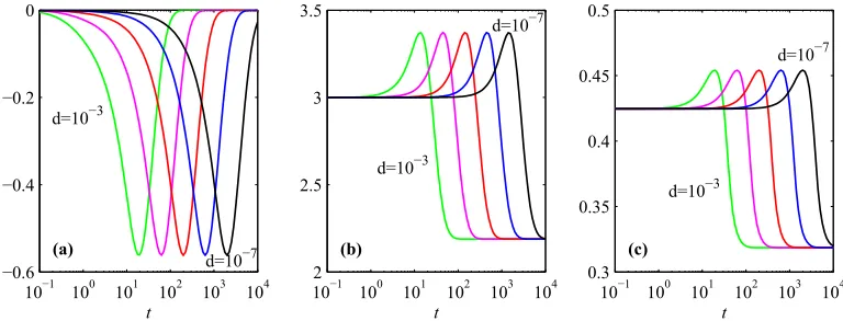
quantity to consider is the ratio of the variance σ to the half-peak width. For this one finds analytically that a Gaussian has 0.425, whereas a quartic has 0.319. Figure 4 shows how these three diagnostics evolve in time. The skewness starts and ends at zero, as expected, but at intermediate times reaches a peak negative value of −0.56, reflecting this difference in the two location measures in Fig. 3. This negative value of skewness is predicted in Sec. II C. The kurtosis similarly starts at 3 and ends at 2.19, as expected, but at intermediate times actually increases to a peak of 3.37. The variance-to-width ratio follows the same pattern as the kurtosis.
These results are interesting in the following two aspects. First, this clearly shows that the stationary PDF is very different from the nonequilibrium PDF. Second, the broadening of the PDF in the intermediate time before reaching the stationary PDF is reminiscent of a cyclic geodesic solution in Ref. [18], suggesting an important role of nonlinear interaction (force) in a geodesic. Detailed discussion on the implications of these results for information change is provided in Ref. [35]. The last point to note about all three diagnostics is how the curves for different values ofdare essentially identical, but offset in time according to a d−1/2 scaling. This is another reflection
of the result derived analytically and discussed in Sec. II C
10−1 100 101 102 103 104
−0.6 −0.4 −0.2 0
t
d=10−3
d=10−7
(a)
10−1 100 101 102 103 104
2 2.5 3 3.5
t
d=10−3
d=10−7
(b)
10−1 100 101 102 103 104
0.3 0.35 0.4 0.45 0.5
t
d=10−3
d=10−7
(c)
FIG. 4. (a) The skewness[(x− x)2/σ]3p dx, (b) the kurtosis[(x− x)2/σ]4p dx, and (c) the ratio of variance to half-peak width.
[image:9.608.111.494.74.221.2] [image:9.608.110.494.564.711.2][see. Eq. (62)] and also seen in Fig.2that the final adjustment time scale for the cubic process scales asd−1/2.
IV. CONCLUSION
We have presented time-dependent PDFs in a cubic nonlinear stochastic process where the frictional force is given by a cubic nonlinearity. Analytically, we applied an instanton method based on a path integral formulation to a nonlinear system in the limit of weak noise (small D) and proposed a new nonlinear time transformation to solve nonlinear instanton (saddle-point) equations. We predicted a PDF which in general involves an integral and elucidated the effect of nonlinear interaction on enhanced dissipation in relaxation processes. Useful local time-dependent PDFs were presented in certain limits (e.g., in the short and long time limits). In particular, a transient PDF in the cubic process was shown to be asymmetric around its peak while the relaxation time tf > tc∼√μD1 in Eq. (62) depends on D, increasing as D decreases. This sharply contrasts a linear stochastic process where transient PDFs are Gaussian and symmetric while the relaxation timetf to the final stationary PDF is independent of the diffusion coefficient D. The D dependence of the relaxation time for a cubic process reflects a close interlinking between space and time in nonlinear relaxation processes. Alternatively, time flows at a different rate depending on the coordinate. We also demonstrated the utility of generalized two-family trigonometric functions in solving nonlinear equations. Numerical simulation of the Fokker-Planck equation revealed detailed evolution of the time-dependent PDF; analytical and numerical results agreed on overall PDF evolution, in particular, transition times for different evolutions (e.g. relaxation timetf) and asymmetry, as noted in Sec. II C and 3. Furthermore, it highlighted that transient PDFs behave drastically differently from the stationary PDFs in regard to the asymmetry (skewness) and kurtosis. Of particular interesting is the settling in to a symmetric and narrow stationary PDF only after undergoing a transient state with asymmetric and broad PDF.
The generality of our methodology and predicted exponen-tial PDF are reminiscent of the possibility of transforming any automonous nonlinear Langevin equation driven by a white noise to the Brownian motion, while our proposed nonlinear time transformation plays a role of random time change: the so-called Lamperti transformation [2,3]. The latter transforms away a nonlinear diffusion coefficient (D) to a constant diffusion (e.g., see Refs. [36,37] and Theorems 7.37 and 7.39 and Remark 7.4, chap. 7 in Ref. [2]). Together with the change of variables, or change of measure (Girsanov transformation) which removes the drift term (i.e.,∂V∂x in our case), the solution to any stochastic equation with time-independent coefficient can be obtained by the Brownian motion (e.g., see Refs. [2,3]). However, since the resulting Brownian motion depends on random time, it is not clear how to calculate transient PDFs by using this method. In comparison, our nonlinear time transformation seems to offer a systematic way of computing the PDFs in different limits. This opens a large scope for future study including the application of our method to other nonlinear stochastic processes. Of particular interest would be the inclusion of a linear (negative) force in the cubic process
to investigate the dynamics of growth, phase transition, and long-term memory. A change of variables would then permit us to examine the Feller-branching process with a logistic growth (e.g., see Ref. [36]). Furthermore, the investigation of the change in information in nonlinear processes in terms of information length [17] is addressed in the accompanying paper [35].
APPENDIX A: PROPERTY OFp(x)=Nexp(−βx4) We first show how to fix N by the unity of the total probability−∞∞ dx p(x)=1:
N−1=
∞
−∞
dx e−βx4
=2
∞
0
dx e−βx4
= 1 2β
−1 4
∞
0
dy y−34e−y
= 1 2β
−1 4
1 4
, (A1)
where the change of the variabley=βx4(dx =14β−14y− 3 4dy)
was used and(z)=0∞dy yz−1e−y is the Gamma function. That is,
p(x)= 2β
1 4
14e
−βx4
.
By using Eq. (A1), we can calculate the second and fourth moments as follows:
x2 =
∞
−∞
dx x2p(x)=2N
∞
0
dx x2e−βx4
= N 2β
−1 4β−
1 2
∞
0
dy y−14e−y
= 34
14β
−1
2 (A2)
and
x4 =
∞
−∞
dx x4p(x)=2N
∞
0
dx x4e−βx4
= N 2β
−1 4β−1
∞
0
dy y14e−y
= 54
14β
−1 =1
4β
−1, (A3)
where(z)=(z−1)(z) was used forz=54 in the last line. From Eq. (A2) and Eq. (A3), we find the kurtosisκ:
κ = x
4
x22 =
1 4
1
4
3
4
2
=2.1884. (A4)
APPENDIX B: PATH INTEGRAL IN EQ. (12) For Gaussian statistics with vanishing first moment, the prescription of the second moment given by Eq. (2) is sufficient. It is simply because all odd moments vanish while even moments can be expressed as a product of second moments. Note that even if the forcing is Gaussian, statistics of x can be Gaussian because of the non-linearity of the dynamical equation. An equivalent way of prescribing the second moment (2) for the Gaussian forcing is to introduce the probability density function for ξ as follows [12,26,33]:
d[ρ(ξ)]=Dξexp
−1 2
dt D−1ξ(t)2
. (B1)
This is a Gaussian distribution forξ(t). The average value of a quantityQis then computed as
Q =
d[ρ(ξ)]Q .
When the average value of a functional ofx (i.e.,Q[x]) is required, the constraint should be imposed thatξ andxsatisfy the original equation (1). This can be done by inserting an identity with aδfunction, which enforces Eq. (1), as
1=
Dx δ
dx dt +
∂V ∂x −ξ
J
∝
DxDx exp
i
dt x
dx
dt + ∂V
∂x −ξ
J, (B2)
whereJ =J[∂ξ∂x] is the Jacobian due to the change of variables for the delta function. Let us show in detail how this is done. Starting from the definition,
Q[x] =
Dξ Q[x] exp
− 1 2D
dt ξ(t)2
=
DξDx Q[x]δ
dx dt +
∂V ∂x −ξ
J
×exp
− 1 2D
dt ξ(t)2
=
DξDxDx Q[x] exp
i
dt x
dx dt
+∂V ∂x −ξ
Jexp
− 1 2D
dt ξ(t)2
=
DxDx Q[x]e−S, (B3)
leading to S given in Eq. (12). In Eq. (B3), Eq. (B2) was used to obtain the third line;J =e−ψ andψ= −3
2μx2 [see,
e.g., Eq. (96)–(97) in Ref. [33], Eq. (2.10) in Ref. [12]] for V(x)=μx4/4 and the Gaussian integral over ξ were used
to obtain the last line. TakingQ[x]=δ(x(tf)=xf)δ[x(0)= x0] gives us Eq. (11). Note that x is a conjugate variable,
which acts as a mediator between the forcingξand dynamical variablex.
APPENDIX C: NONLINEAR TRANSFORMATION [EQ. (18)] Let us consider a homogeneous cubic equationdx
dt = −μx
3.
The usual way of solving this equation is to separate variables and integrate to obtain
x(t)= x0 1+2μt x02
, (C1)
where the initial conditionx(t =0)=x0is used. To elucidate how the nonlinear transformation defined in Eq. (18) works, we rewrite dxdt = −μx3as follows:
0= dx dt +μx
3 =x2
dx dτ +μx
. (C2)
The solution to Eq. (C2) isx(τ)=x0e−μτ wherex
0 =x(τ =
0)=x(t =0). To obtain x(t), we use x(τ1)=x0e−μτ1 in
Eq. (25):
t =
τ
0
dτ1
1 [x(τ1)]2 =
1 2μx02(e
2μτ− 1)
= 1 2μx2
0
x2 0
[x(t)]2 −1
. (C3)
Solving Eq. (C3) forx(t) gives the same solution [Eq. (C1)].
APPENDIX D: GENERALIZED TWO-FAMILY TRIGONOMETRY FUNCTIONS
The generalized sine function with two parameters p,q, where p >1 and q >1, is defined through its inverse function [34]
arcsinp,q(x)=
x
0
dt(1−tq)−1/p, (D1)
where x =[0,1]. Note that when p=q =2, Eq. (D1) recovers the definition of the usual arcsin(x). When x =1, Eq. (D1) defines the generalizedπp,q as
arcsinp,q(1)=
1
0
dt(1−tq)−1/p =πp,q
2 , (D2)
which again recovers π/2 when p=q=2. We note that sinp,q(x) is a monotonically increasing function ofx, mapping [0,1]→[0,πp,q/2], and Eq. (D1) can also be written in terms of Gaussian hypergeometric function.
The (p,q)-cosine is defined as
cosp,q(x)=
dsinp,q(x)
dx = {1−[sinp,q(x)] q}1/p,
(D3)
wherexis a real number. Hence, cosp,q(x) is strictly decreasing on [0,πp,q/2], cosp,q(0)=1, cosp,q(πp,q/2)=0 and satisfies the following identity:
|sinp,q(x)|q+ |cosp,q(x)|p=1, (D4)
APPENDIX E: DERIVATION OF EQ. (32)
To show the identity Eq. (32), we let the left-hand side of Eq. (32) beI1and reexpress it as follows:
I1 ≡
z
0
dz1 1 1−z315/3
(E1)
=
z
0
dz1
1−z31
1−z135/3 + z31
1−z315/3
(E2)
≡I0+
z
0
d[ 1−z31−2/3]z1
2 (E3)
=I0+
1 2
z (1−z3)2/3 −
1 2
z
0
dz1
1
1−z3 1
2/3 (E4)
=I0+
1 2
z (1−z3)2/3 −
1 2I0=
1 2I0+
1 2
z
(1−z3)2/3 (E5)
= 1 2
z
0
dz1 1−z31 −2/3
+z(1−z3)−2/3
, (E6)
obtaining Eq. (32) in the text. Here I0 in Eqs. (E3)–(E5) is
defined as
I0≡
z
0
dz1 1 1−z312/3
, (E7)
and integration by parts is used to obtain Eq. (E4) from Eq. (E3).
APPENDIX F: FORy−γ >0 In this case, we obtain from Eq. (38) and Eq. (25)
t = 1 6μB23
I0, (F1)
where
I0= yf
1
dy
y23
1 (y−γ)23
. (F2)
Here y=e6μt and yf =e6μτf. Similarly, Eq. (38) can be written as
Seff =
μB43
3D I1= μ
6D{6μtf|αB| +3B
4
3[y1/3(y−γ) 1 3]yf
1 },
(F3)
I1 =
yf
1
dy y
1 3
(y−γ)23
. (F4)
In the second line in Eq. (F3), we used Eq. (F1) and the following identity (similar to that used in AppendixC):
I1=
1 2
γ I0+3[y1/3(y−γ) 1 3]yf
1
. (F5)
APPENDIX G: DERIVATION OF EQ. (45) We rewriteI0in Eq. (42) in terms ofI1in Eq. (44) as
I0= yf
1
dy y
−2 3
(γ−y)23
= 1
γ[I1+J], (G1)
where
J =
yf
1
dyy−23(γ −y) 1 3
=3
[y13(γ−y) 1 3]yf
1 +
1 3
yf
1
dyy13(γ−y)− 2 3
=3[y13(γ−y) 1 3]yf
1 +I1. (G2)
By using Eq. (G2) in Eq. (C1), we obtain
γ I0=2I1+3[y 1 3(y−γ)
1 3]yf
1 ,
which gives Eq. (45).
APPENDIX H: ALTERNATIVE DERIVATION OF THE RELAXATION TIME TO THE STATIONARY PDF To estimate the relaxation time to the stationary PDF, we letr=r(0)+r(1) in Eq. (61) by assuming a smallQ−1 and find
r=
2D μ
1
4
− 3
42μtf .
By comparing the two terms in r above, we conclude that the critical timetcrequired to relax into the equilibrium PDF satisfies
tf > 9
32√2Dμ (≡tc). (H1)
[1] H. Risken,The Fokker-Planck Equation: Methods of Solution and Applications: Methods of Solutions and Applications, 3rd ed. (Springer, New York, 2013).
[2] F. Klebaner, Introduction to Stochastic Calculus with Applications (Imperial College Press, London, 2012), ch. 5.5.
[3] C. Gardiner,Stochastic Methods, 4th ed. (Springer, New York, 2008), ch. 4.4.
[4] H. Haken,Information and Self-organization: A Macroscopic Approach to Complex Systems, 3rd ed. (Springer, New York, 2006), pp. 63–64.
[5] B. R´enyi,Proceedings of the Fourth Berkeley Symposium on Mathematical Statistics and Probability, edited by J. Neyman (University of California Press, Berkeley, 1961), p. 547. [6] A. D. Wissner-Gross and C. E. Freer, Phys. Rev. Lett.110,