DE Mosaicing using Matrix Factorization Iterative Tunable Method

International Journal of Innovative Technology and Exploring Engineering (IJITEE) ISSN: 2278-3075, Volume-9 Issue-1, November 2019

DE-Mosaicing using Matrix Factorization Iterative

Tunable Method

Shabana Tabassum, SanjayKumar C. Gowre

Abstract-A color image is captured though the single image sensor and it is named as the mosaicked image and this is obtained through the CFA where the pixels are arranged such that any one of the color from the given color component is recorded at every pixel. De-mosaicingis absolute reverse of mosaicking, where the process is to reconstruct the full color image from the given incomplete color samples. In past several methods of de-mosaicing have been proposed however, they have many shortcomings such as computational complexity and high computational load, not matching the original images. Hence we have proposed a methodology named as MFIT i.e. Matrix factorization Iterative Tunable approach, the main aim of this methodology is to improvise the reconstruction quality. In order to achieve the better reconstruction quality we have used the MFIT algorithm at each iteration this helps in avoiding the image artifacts and it is achieved through the image block adjustment also it reduces the computational load. Moreover in order to evaluate the proposed algorithm we have compared it with nearly 12 algorithm based on the value of PSNR and SSIM, the theoretical results and comparative analysis shows that our

algorithm excels compared to the other existing method of de-mosaicing.

Keyword: De-mosaicing, MFIT, Matrix Factorization, Iterative Tunable.

I. INTRODUCTION

Nowadays most people share their picture of various events with people through the internet easily, the demand of DSLR has become widely popular and it has become one of the indispensable device in work as well as life. Moreover, in this entire scenario, the image resolution is one of the eminent aspect for the standard quality of image[1]. Almostall the Digital Camera have been designed through the single color CMOS, whichis masked with the CFA(Color filter array), the CFA are used for capturing the single color at every pixel [2].De-mosaicing is defined as the process of color image reconstruction through the estimation of missing samples of color; mosaic is the word which is used reconstruction of the original scene in its true color[3]. De-mosaicing is also known as the CFA interpolation, so in other words it refers to the reconstruction problem of the image from the samples of CCD(Charge Coupled Device)[4], the reconstruction takes place based on the three color image without the complete information of image. In other words using the de-mosaicing method, the detail color information can be maintained.

Revised Manuscript Received on November 05, 2019.

Shabana Tabassum, Associate Professor, Dept of E&CE, KBN College of Engineering, Kalaburagi-585104.

Email:[email protected]

Dr. SanjayKumar C. Gowre, Professor, Dept of E&CE, BKIT, Bhalki-585328 Email: [email protected]

Typically the CFA constitutes the color sensor at every position of the pixel, hence the color information are measured at every image pixel, for instance if we want to capture the color image it is eminent to either capture the other two color or reconstruct through the data. One of the widely available CFA pattern is named as Bayer CFA[5], it uses the three distinctive primary colors as the filter sensors in order to obtain and reconstruct the RGB data of given scene. In case of low cost production,the digital color camera uses the single chip of CCD; this is done since the single kind of color data can be acquired through each pixel. Moreover in order to re-construct the high visual quality as well as high-resolution images, the CFA has to be –placed between the sensor and the lens, later the high quality images are reconstructed. Moreover, it has been noticed that the production cost is much more complicated and high, hence deployment is avoidable. Moreover, if single piece of the CSA is used then it can achieve only insertion and the information collected is not complete hence the image might appearance.

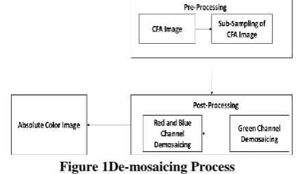
Figure 1De-mosaicing Process

The above diagram shows the typical de-mosaicing process, it has three different blocks, first block presents the pre-processing, this block shows the Initial stage for the data processing , In here the images are sub-sampled into three distinctive channels and it follows the random pattern which contains the three primary color i.e. RGB. Second block contains the Post-processing, through this block the demosacing initiates with the green color since it is the largely available color in the CFA and it is made as the guide channel also it is first channel, this in terms results in the absolute image as the output.

The main aim of de-mosaicing is interpolating the missing green, red and blue pixels from the given color this is achieved so that the reconstructed image is as close as to the original image. Moreover, the CC(Computational Complexity) of de-mosaicing is required to be on the lower side for being the cost effective. However, there are many constraints as similar as any other image processing i.e. modelling of the correlation among these three colors, these colors plays important role in

These colors share almost same characteristics such as edge location and texture, ignorance of such dependency causes the annoying artifacts ,these artifacts are mainly due to the mis registration. Moreover in past several technique has been proposed which has been discussed in the literature survey section. Mainly these methods were proposed to achieve the higher quality image through the exploitation of interplanecorrelation;moreover, the primal issue is finding the best tradeoff between the computational cost and quality of image. These methods were parted into two distinctive categories i.e. iterative[6] and non-iterative[7]. Non-iterative technique is based on the edge directed interpolation for improvising the performance of construction, here the exploitation takes place through the estimation of local covariance information[8] and local gradients[9] and it is based on either difference rule[10] or ratio rule of color[11]. Moreover in [12] ration rule of color were enforced through iterative updating the three color channels, similarly in POCs technique were used for refining the blue and red plane though enforcing the dual convex set constraints and it is observed that iterative approach are more capable of achieving the high quality image.

Hence, in this paper we have proposed a methodology based on the matrix factorization, the main advantage of matrix factorization approach is that it acquires the comparatively less computational load and requires the less memory than the other methodology of image reconstruction. Moreover, Matrix Factorization also has few drawbacks due to the particular type of defining image block set, like otherde-mosaicing reconstruction method Matrix factorization can be implemented using the stride or non-stride image blocks. Striding image block can reduce the block artifacts but has the shortcomings as it comes with high computational cost; the computational cost is more due to the huge number of image blocks involved.Moreover, partition made up of non-striding image block has the lower computational cost, but this causes the block artifacts.Hence, in both cases the three are limitation and cannot be applicable for real life application. Hence, in this paper,the iterative tunable approach has been introduced and methodology is named as MFIT (Matrix Factorization), this particular research work has following contribution:

With the help of matrix factorization we introduce a methodology named as MFIT i.e. Matrix Factorization with iterative tunable approach.

It reduces the computational cost upto the large extend. It promotes the non-striding image block partition, as it requires the low value singular matrix.

In this at each iteration, MFIT is applied for solving the optimization issue.

One of the main advantage of MFIT is that it suppresses the block artifacts and at the same time it reduces the computation load and these two are achieved through the iterative tunable approach.

This helps in reconstruction of image with the high quality with less computational cost

Our research work is organized in such a way that first section starts with the theoretical definition of de-mosaicing and basic of it ,in the same section later part shows the different virtue related to it, first section ends by briefing the contribution of this research work. Second section describes

the various exsitng work and their survey, this in terms helps in designing the methodology. Third section shows the proposed methodology along with the flow chart and mathematical notation. Fourth section presents the evaluation of algorithm along with the comparative analysis.

II. LITERATURE SURVEY

In past several de-mosaicing algorithm has been presented some of them are discussed in this particular section, here brief survey of several existing system has been presented and it has been helpful in designing the proposed methodology at first The process in [12] suggested an universal de-mosaicing technique which reconstructs images from various types of CFAs(Color Filter Arrays) for allowing the comparison of the quality of image. This technique calculates the chrominance components through two mechanism(edge-sensing and distance-related weighting to estimate the confidence stages of the inter-pixel chrominancemechanism, and pseudo-inverse-based approximation from the mechanism in a window) and there is reconstruction of the colors through linear transformation, that joins the real Color Filter Arrays(CFA) color component.There are two approximation of the chrominance

components. A collection of de-mosaicking

algorithm,e.g.[13,14] predicts that the ratio of color of an article that is uniformly colored is constant w.r.t(with respect to) the condition of lighting inside that the article is captured. These type of algorithm first include the G channel (e.g in terms of an edge-directed interpolation and bilinear interpolation), after that there is estimation of B and R channels on consider the B-to-G ratio and R-to-G ratio. Laplacian filter is utilized in [15] to include the missing channel vertically or horizontally, selecting a direction to reserve edges. In [16] authorssuggested an developed method dependent on high-order interpolation, utilizing the Sobel operator to measure the gradients and to detect edges. Some de-mosaicing methods exploit ANN (artificial neural network),e.g.[17]whereas the training pictures learnt offline that are utilized to rebuild misused color of initial pictures. The paper [18] shows the termed sparse based radial base function network for the image of color de-mosaicing: it presents a sparse model of the input image and measure the reconstruction of the error. Sparse de-mosaicing encoders is utilized to pre-train the coatings of a depth of a neural network, in order to decrease the complexity of system complexity inexcursing a network a from mark.

International Journal of Innovative Technology and Exploring Engineering (IJITEE) ISSN: 2278-3075, Volume-9 Issue-1, November 2019

The multi-level gradient method shows in[20] improves and extends the algorithm [21]: then a first de-mosaicing phase, the multi-level gradient methods corrects the wrong interpolations, consideration of chrominance connection among the channels. A polynomial interpolation-based de-mosaicing procedure that is suggested in [22].There are three steps that consist of this method:(i)generation of the predication error on the base of on the PI(polynomial interpolation),(ii)classification of edge that is dependent on the differences of color (ii) to improve the quality of the reducing image the artifacts.

In[23] a process dependent on an advanced NML(non-local mean) filter is presented. The NML filter reflects similar patches, other than similar pixel, to rebuild missed color pixels.A 3-dimensional distance locality that is described to favor the choice of pixels through a structure Same to that of the lost pixels in the area. Some process work under the frequency domain. For example, the efforts clearly suggested an adaptive filtering process to reserve high-frequency details, and consequently stores a higher image quality. Wavelets are utilized in to approximate edge directions, and in [24] to develop the performance of color filter arrays(CFA).In particular, in here the three-step process are implemented by authors(i)Comparison of edge in sub-bands,(ii)transformation of wavelets to extract horizontal and vertical edge information and (ii)downsampling the channels of color. The work in [25] shows a minimization method that joins spatial and spectral representation of original image to resolve the inverse problem of improving samples of missing color from the data of CFA. The representation of spectral sparse defines spectral connection and outcomes from formation model of physical image, whereas the representation of spatial sparse is created on a component analysis of adaptive principal and define the image of local spatial structures.

In a brief survey of demosiaicng algorithm can be concluded by noting the point that all these methods have several drawbacks such high computational load, computational complexity or the poor reconstruction, hence we have developed a novel de-mosaicing methodology based on the matrix factorization which is discussed in detail in next section.

III. PROPOSED METHODOLOGY

De-mosaicing is consideredto be one of the eminent area in the image processing, and reconstruction of images has been widely popular due to high demand and extensive use of social media. Throughout the above section, we have observed that every other technique lacks from one or other issue, hence in this we have designed a novel method for the reconstruction of image. Our method is named as MFIT i.e. Matrix Factorization Iterative Tunable.

Matrix Factorization method

Let usconsider an image by 𝑋 × 𝑌 , then the forward model can be represented by the below equation.

Where 𝑈𝐷 signifies the under sampled data and 𝐺𝑛signifies

the Gaussian noise,𝑈𝑜 is the under sample operator where 𝑈𝑜 :𝐷𝑋𝑌𝐷 ⟼ 𝐷𝑍𝐷 and also 𝐺𝑛𝜖 𝐷𝑍𝐷, 𝑍 < 𝑋𝑌, similarly

acquisition can be defined as : 𝑋𝑌/𝐷.In order to form the matrix factorization, the given underlying image is parted into the two image block i.e. stride and non-stride, the image blocks within the Ω is denoted by Ω and each one is described as 𝑟 ∈ 𝛺, r = {1,2,……… Ω } In a given set of image blocks, an image is parted into the various ways, this can be done by displacing the partition by various amount of pixels with the every dimensions. Displacement in shifts can be denoted by using𝐷𝑖𝑠𝑐Ω.these image blocks have the

dimensions of𝑥 × 𝑦.

Let us consider 𝑀𝑟: 𝐷𝑋𝑌𝐷 ⟼ 𝐷𝑍𝐷 as the linear operator,

which has been, extracted from the given𝑝image data. This data corresponds to the 𝑟𝑡𝑕_{image block of segregatedΩ, this}

in terms generates the matrix𝑀𝑟(𝑝). The inner product 𝐸, 𝐹 _𝐷𝑥𝑦 ×𝐷 = 𝑟𝑒𝑐𝑜𝑛(𝑡𝑟(𝐸𝐻 𝐹)) then the 𝑀_𝑟 ∗ satisfies the below equation.

𝑀_𝑟 𝑃 , 𝑄 _𝐷𝑥𝑦 ×𝐷= 𝑋, 𝑀_𝑟 ∗(𝑄) ₂ (2)

𝑃 ∈ 𝐷𝑋𝑌𝐷 _{And Q ∈ 𝐷}𝑋𝑌𝐷 _{, from the above equation the}

linear operator can be defined as 𝐿Ω: 𝐷𝐷𝑋𝑌→𝑃, where 𝑋 = 𝐷 Ω ×𝐷×𝑥𝑦_{, the 𝐿}

Ω𝑃 component is given by below

equation.

[𝐿Ω𝑃]𝑟= 𝑀𝑟(𝑃) (3)

The inner product is given by the below equation where r = {1,2,……… Ω } i.e. equation 4 and the norm is given as in equation 5

𝑃, 𝑄 𝑃 = 𝑅𝑒𝑐𝑜𝑛(𝑡𝑟( 𝑃𝑟𝑄𝑟𝐺 )) Ω

𝑞=1

(4)

Norm is given as where 𝑃𝑟, 𝑄𝑟𝜖𝐷𝑥𝑦 ×𝐷

𝑃 𝑃 = ( 𝑃, 𝑃 𝑃)1/2 (5)

Another adjoin 𝐿∗Ω: 𝑃 → 𝐷𝐷𝑥𝑦 is said to be the linear

operator which satisfies the below equation.

𝐿Ω𝑃, 𝑄 𝑝= 𝑃, 𝐿Ω𝑃 2 (6)

For any Q∈ P and P∈ 𝐷𝑑𝑥𝑦_{, this can be defined by the}

below equation.

𝐿∗Ω𝑄 = 𝑀𝑟∗𝑄𝑟 Ω

𝑟=1

(7)

Since all the partition contains only non-stride image blocks which can cover entire image, then we have the following equation, since this problem is considered as the NP hard problem and the matrix is nonconvex function, rank of given matrix is approximated using the Matrix norm

𝑃 = 𝐿∗Ω(𝐿Ω𝑃)

𝑄 = 𝐿Ω(𝐿∗Ω𝑄)

(8)

Let there be any matrix Z which belongs to 𝐷𝐺_{𝑛 1}×𝐺_{𝑛 2 as} 𝜎(𝑍) 𝑝 = 𝑍 𝑆𝑝 (9)

𝜎(𝑍) is said to be the singular values of given vector Z, based on primal dual algorithm [28] the image-block based matrix factorization can be defined in terms integrated norm i.e. for any element P∈ p is defined as below

𝑃 1,1= 𝑃𝑟 𝑆1 Ω

𝑟=1 (10)

Similarly the optimization problem can be formulated as in the below equation, λ is said to be the regularized parameter which maintains the trade-off between the constancy of data and matrix factorization. Below equation presents the generalized version to recover the Matrix Factorization image block from the given under-sampled measurement , assuming the segregation Ω of non-striding/

𝑃 = arg 𝑚𝑖𝑛 1

2 𝑈𝐷− 𝑈𝑜𝑃 2 2_{+ 𝜆 𝐿}

Ω 𝑃 1,1

𝑃𝜖 𝐷𝐷𝑋𝑌

(11)

In the above equation i.e. equation 11 𝜆 is considered as the regularization parameter which helps in balancing the trade of among data fidelity and matrix factorization image 𝑝 . the above equation represents formulation for recovering the matrix factorization p assuming that Ω of non striding, covering image blocks.

Optimization through Iterative Tunable

We use the sparsity driven [29] to solve the above equation, this reduces the order of surrogate functions. Iterative tunable process is applied, our algorithm iteratively reduces the

𝑓(𝑃, 𝑃0)= 𝛼

2 𝑃 − 𝑆 2

2_{+ 𝜆 𝑃𝐿}

Ω 1,1 (12)

Here, 𝑆 = 𝑃0+ 1 𝛼𝑈𝑜

𝐻_(𝑈

𝐷− 𝑈𝑜𝑃0)and 𝛼 ≥ 𝜆𝑚𝑎𝑥(𝑈𝑜𝐺𝑈𝑜).

The implementation of algorithm is done by minimizing the function in the given equation. This can be written as below equation:

𝑃 1,1 =

𝑚𝑎𝑥 𝜓, 𝑃 𝑃 𝜓 ∈ 𝑀𝐹∞,∞

(13)

𝑀𝐹∞,∞is matrix factorization 𝑃

= arg 𝑚𝑖𝑛 1

2 𝑃 − 𝑆 2 2₊ 𝜆

𝛼

𝑚𝑎𝑥

𝜓 ∈ 𝑀𝐹∞,∞ 𝑃, 𝐿Ω ∗ _𝜓

2

𝑃 ∈ 𝐷𝐷𝑋𝑌

(14)

Later our algorithm makes sure that segregatedΩ remains constant throughout the iterations and the updation of

segregation is done in each segregation, this minimizes the block artifacts. Moreover, each image block is independent from one another. Moreover further the optimization is done.

𝑀𝐹∞,∞ = Ψ ∈ 𝜒: Ψ𝑟 𝑤∞ ≤ 1, ∀𝑟= 1,2, … … , Ω (14)

The above definition along with the ad joint operator 𝐿∗Ω the

minimized version of the above equation can be represented as

P

= 𝑎𝑟𝑔 min Pϵ𝐷 𝑋𝑌𝐷

1

2 𝑃 − 𝑆 2 2

+ 𝜆 𝛼 max Ψ∈MF∞ ,∞

𝐿∗Ω 𝜓, 𝑃 2

(15)

Through the above equation we observe that the objective function is concave when it comes to Ψconvex when it comes to X, hence this causes the generation of minimax point, at the minmax point the equation tend to attain the common value. Hence the below equation can be written

ℒ P , Ψ = max Ψ∈MF∞ ,∞

min

x∈𝐷 𝑋𝑌𝐷ℒ P, Ψ

(16)

The above equation identify the POF (Primal Objective Function) which is depicted in below equation

𝜌 P = max Ψ∈MF∞ ,∞

ℒ P, Ψ

=1

2 p − s 2 2

+⋋

𝛼 𝐿ΩP 1,1

(17)

Similarly DOF(Dual Objective Function) is given as 𝑊 Ψ = min

P∈𝐷 𝑋𝑌𝐷ℒ P, Ψ

=1 2 𝑆 2

2_{− 𝑆 −}⋋ 𝛼𝐿Ω

∗ _𝜓 2 2

(18)

Min of P can be known by knowing the max of Ψ and this is achieved by considering the below equation.

P

= 𝑆 −⋋ 𝛼𝐿Ω

∗ _𝜓 (19)

From 18, Using the equation 5, 6, 7, 8

max

Ψ∈MF_{∞ ,∞}𝑊 Ψ =Ψ∈MFmin∞ ,∞ 1 2 𝑆 −

⋋ 𝛼𝐿Ω

∗ _𝜓

2 2

= min Ψ∈MF∞ ,∞

⋋

𝛼𝐿Ω𝑆 − Ψ 𝜒 2

(20)

Max of (18) is found through the projection of ⋋

𝛼𝐿Ω𝑆 to the MF∞,∞, this projection is achieved using the projection of

every ⋋

𝛼𝐿Ω𝑆 components onto the given unit norm ball 𝑈𝑁𝑀𝑊_∞. Moreover the projection through 𝑈𝑁𝑀𝑊_∞. is

International Journal of Innovative Technology and Exploring Engineering (IJITEE) ISSN: 2278-3075, Volume-9 Issue-1, November 2019

𝑃𝑟𝑜𝑗𝑈𝑁𝑀_{𝑊 ∞} ⋋ 𝛼 𝐿Ω𝑆 𝑟

=⋋

𝛼𝑇𝑟 min σ LΩS r , ⋋ α Or

c

= Ψ𝑞

(21)

Hence, from 19 and 21 we get equation 22

=> P = 𝒫roj𝑟∗ Ω

𝑞 =1

𝑇𝑟𝑑𝑔 𝑆⋋ 𝛼

𝜎 𝐿Ω𝑆 𝑟 Orc

(22)

Equation 23 represents the operator which is applied on the singular vector.

𝑆⋋ 𝛼

𝜎 𝐿Ω𝑆 𝑟 =(max( (𝑃𝑟)-

𝛽,0)

(23)

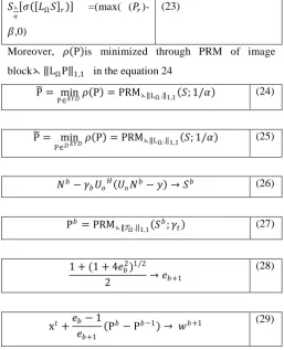
Moreover, 𝜌 P is minimized through PRM of image block⋋ LΩP 1,1 in the equation 24

P = min

P∈𝑋𝑌𝐷𝜌 P = PRM⋋ LΩ. 1,1 𝑆; 1/𝛼 (24)

P

= min

P∈𝐷 𝑋𝑌𝐷𝜌 P = PRM⋋ LΩ. 1,1 𝑆; 1/𝛼

(25)

𝑁𝑏− 𝛾𝑏𝑈𝑜𝐻 𝑈𝑜𝑁𝑏− 𝑦 → 𝑆𝑏 (26)

P𝑏_{= PRM}

⋋ 𝒯_Ω. _1,1 𝑆𝑏; 𝛾𝑡 (27)

1 + (1 + 4𝑒𝑏2)1/2

2 → 𝑒𝑏+1

(28)

x𝑡+𝑒𝑏− 1 𝑒𝑏+1

P𝑏_{− P}𝑏 −1 _{→ 𝑤}𝑏 +1 (29)

Moreover eq.22shows the reconstruction of image, iterations, from eq.25 to 27 shows the Iterative tunable approach iteration to solve the equation 11, and it is achieved using the given fixed partition.

Matrix Factorization based on stride image block Lets consider the image block of dimension 𝑢𝑋 𝑣 which is used for covering the image matrix 𝑈𝑋𝑉, these image block are stride through the 𝑆𝐼 pixels and these are stride though NSI pixel, hence the whole striding image block which cover the image are given by the below equation, SIB is the Striding Image Block,

𝑆𝐼𝐵 = 𝑈 + 𝑢 1 − 𝑔

𝑁𝑆𝐼

𝑉 + 𝑣 1 − 𝑕 𝑆𝐼

(30)

Lets consider L as the non-striding partition this corresponds to the P striding image block , then the optimized problem is given in the below equation

P

= 𝑎𝑟𝑔 min

Dϵ𝐷 𝑋𝑌𝐷 0.5 𝑈𝐷− 𝑈𝑜P 2

2₊

⋋. 𝑔𝑕 𝐿ΩP 1,1 Ω ∈Γ

(31)

Matrix factorization with iterative tunable approach Earlier part of the section shows that the fixed partition remain constant throughout the iterations, however in here through the iterative tunable approach updates the partition in every iteration, this causes the reduction in artifacts. The main advantage with iterative tunable approach is that it achieves the time invariant even without stride image block and this helps in less computational consumption.

IV. RESULT AND ANALYSIS

In this section, our methodology is evaluatedto prove the efficiency of methodology, in order to prove we have simulated in-house by using g the MATLAB as a language and ran it on the windows workstation with i5 processor along with 2 GB NVidia Graphics and packed with 8 GB RAM.In order to evaluate our proposed methodology i.e. MFIT, we have used the two standard color image datasets namely IMAX and Kodak datasets, these two datasets were used for the benchmark comparison. IMAX dataset has 18 images of size 500x 500 pixels and the Kodak dataset consists of 12 image of same size.

Our methodology were compared with 13 different methodology based on the two parameter i.e. PSNR and SSIM. PSNR and SSIM are the two well-knownimage quality matrices.Moreover, there is no particular rule for selecting the PSNR or SSIM.

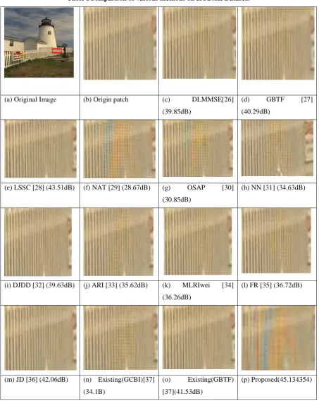
PSNR is calculated using the formula and it is computed through taking square peak value in the given image and divided by the MSE(Mean Square Error), it is used for measuring the image quality after the reconstruction process. PSNR is the error metrics, which is used for comparing the compression quality of the image. The below table shows the comparison analysis based on the PSNR, the image is taken from the Kodak Dataset, these comparison takes place with 13 different algorithm. In comparison with the other algorithm, MFIT possesses the PSNR value of 45.13 db. Higher PSNR indicates the better reconstruction. In case of lossy image when the bit depth is 8 bit, typical value of PSNR is between 30 db and 50db.

SSIM

it employs the modified measure of the spatial correlation between the test images and the pixel of reference, this in terms quantifies the image structural degradation. It predicts the subjective along with sophisticated QA algorithm.

Table 1Comparison of various methods on KODAK Datasets

(a) Original Image (b) Origin patch (c) DLMMSE[26]

(39.85dB)

(d) GBTF [27]

(40.29dB)

(e) LSSC [28] (43.51dB) (f) NAT [29] (28.67dB) (g) OSAP [30]

(30.85dB)

(h) NN [31] (34.63dB)

(i) DJDD [32] (39.63dB) (j) ARI [33] (35.62dB) (k) MLRIwei [34] (36.26dB)

(l) FR [35] (36.72dB)

(m) JD [36] (42.06dB) (n) Existing(GCBI)[37] (34.1B)

(o) Existing(GBTF)

[37](41.53dB)

International Journal of Innovative Technology and Exploring Engineering (IJITEE) ISSN: 2278-3075, Volume-9 Issue-1, November 2019

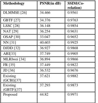
Table 2 shows the comparative analysis based on PSNR and SSIM with different methodologybased onimax dataset, in here we observe that the PSNR value of PSNR is 44.82 and SSIM is 0.9971, this shows that proposed methodology performs better than the other existing technique.

Table 2 comparison analysis of different methodology

Methodology PSNR(in dB) SSIM(Co-relation)

DLMMSE [26] 34.466 0.9561

GBTF [27] 34.376 0.9763

LSSC [28] 36.148 0.9854

NAT [29] 36.254 0.9631

OSAP [30] 33.047 0.9652

NN [31] 40.603 0.9925

DJDD [32] 36.927 0.9868

ARI[33] 37.749 0.9905

MLRIwei [34] 36.894 0.9866

FR [35] 37.449 0.9822

JD [36] 36.532 0.9676

Existing (GCBI)[37]

37.621 0.9882

Existing (GBTF)[37]

37.293 0.9873

Proposed 44.82 0.9971

KODAK DATASET

Table 3 shows the comparative analysis of different techniques with the Kodak datasets, the below result is generated from the average value of Kodak dataset. The average PSNR value of 24 images are 45.58 db which is better the other state of art technique and existing and average SSIM value of SSIM value is comparatively higher than other technique. The comparative analysis of Kodak dataset indicates that MFIT performs better than the other technique.

Methodology PSNR SSIM(Co-relation)

DLMMSE [26] 40.11 0.9858

GBTF [27] 40.623 0.9887

LSSC [28] 41.445 0.9936

NAT [29] 37.714 0.9818

OSAP [30] 39.165 0.99

NN [31] 40.603 0.9925

DJDD [32] 41.45 0.9868

ARI[33] 39.749 0.9937

MLRIwei [34] 39.749 0.9905

FR [35] 39.171 0.99

JD [36] 41.002 0.9923

Existing (GCBI)[37] 42.041 0.9941

Existing (GBTF)[37] 42.122 0.9944

proposed 45.58 0.9969

V. CONCLUSION

In this paper we have presented a novel, efficient and fast de-mosaicing methodology named MFIT i.e. Matrix factorization Iterative Tunable approach which provides the similar level of reconstruction when compared to the striding image block based matrix factorization in terms of quality of the image . Moreover, apart from the better

reconstruction when compared to the other similar methodology is that it also reduces the computational load and computational complexity. The MFIT technique suppresses the artifacts with the retention of convergence rate. The experimental analysis and results shows that our algorithm outperforms the different state- of – art technique including the existing system in terms of PSNR.

Although MFIT performs better than the other technique, it is still in infancy way of using matrix factorization technique with iterative approach and still there needs enormous research in order to implement. Moreover, performance can be improved and also it is interesting to see how our algorithm performs with other parameter with the different constraints.

REFERENCE

1. R. Reulke and A. Eckardt, "Image quality and image resolution," 2013 Seventh International Conference on Sensing Technology (ICST), Wellington, 2013, pp. 682-685.

2. R. Lukac and K. N. Plataniotis, "Color filter arrays: design and performance analysis," in IEEE Transactions on Consumer Electronics, vol. 51, no. 4, pp. 1260-1267, Nov. 2005.

3. D. Su and P. Willis, "De-mosaicing of color images using pixel level data-dependent triangulation," Proceedings of Theory and Practice of Computer Graphics, 2003., Birmingham, UK, 2003, pp. 16-23. 4. C. Chang, J. D. Segal, A. J. Roodman, R. T. Howe and C. J. Kenney,

"Multiband charge-coupled device," 2012 IEEE Nuclear Science Symposium and Medical Imaging Conference Record (NSS/MIC), Anaheim, CA, 2012, pp. 743-746.

5. D. Wang, G. Yu, X. Zhou and C. Wang, "Image demosaicking for Bayer-patterned CFA images using improved linear interpolation," 2017 Seventh International Conference on Information Science and Technology (ICIST), Da Nang, 2017, pp. 464-469.

6. Chung-Yen Su, "Highly effective iterative de-mosaicing using weighted-edge and color-difference interpolations," in IEEE Transactions on Consumer Electronics, vol. 52, no. 2, pp. 639-645, May 2006.

7. Petrova, Xenya&Glazistov, Ivan &Zavalishin, Sergey &Kurmanov, Vladimir &Lebedev, Kirill &Molchanov, Alexander &Shcherbinin, Andrey &Milyukov, Gleb&Kurilin, Ilya. (2017). Non-iterative joint de-mosaicing and super-resolution framework. In Proc. Electronic Imaging'2017.

8. X. Li and M. Orchard, “New edge directed interpolation,” IEEE Trans. Image Process., vol. 10, no. 10, pp. 1521–1527, Oct. 2001.

9. J. F. Hamilton Jr. and J. E. Adams, “Adaptive color plane interpolation in single color electronic camera,” U.S. Patent 5 629 734, May 1997. 10. S.-C. Pei and I.-K. Tam, “Effective color interpolation

11. inCCDcolor filter arrays using signal correlation,” IEEE Trans. Circuits Systems Video Technol., vol. 13, no. 6, pp. 503–513, Jun. 2003.

12. R. Kimmel, “De-mosaicing: Image reconstruction from CCD samples,” IEEE Trans. Image Process., vol. 8, no. 9, pp. 1221–1228, Sep. 1999. 13. Zhang C, Li Y, Wang J, Hao P (2016) Universal demosaicking of

color filter arrays. IEEE Trans Image Process 25(11):5173–5186. 14. Duran J, Buades A (2015) A demosaicking algorithm with adaptive

inter-channel correlation. Image Process Line 5:311–327. https://doi.org/10.5201/ipol.2015.145. http://demo.ipol.im/demo/145/. 15. Pei SC, Tam IK (2003) Effective color interpolation in ccd color

filter arrays using signal correlation.IEEE Trans CircSyst Vid Technol 13(6):503–513.

16. Chung KH, Chan YH (2010) Low-complexity color de-mosaicing algorithm based on integrated gradients. J Electr Imaging 19(2):021104–021104.

17. Baek M, Jeong J (2014) De-mosaicing algorithm using high-order interpolation with sobel operators. In:Proc. of the World Congress on engineering and computer science

18. Wang YQ, Limare N (2015) A fast C++ implementation of neural network backpropagation training

5:257–266. https://doi.org/10.5201/ipol.2015.137. http://demo.ipol.im/demo/137/.

20. Prakash VS, Prasad KS, Prasad TJC (2016) Color image de-mosaicing using sparse based radial basis function network. Alexandria Eng J 21. Wu J, Timofte R, Van Gool L (2016) De-mosaicing based on

directional difference regression and

22. efficient regression priors IEEE transactions on image processing: a publication of the IEEE signal

23. processing society

24. Lee K, Jeong S, Choi Js, Lee S (2014) Multiscale edge-guided demosaicking algorithm. In: The 18th _{IEEE International symposium}

on consumer electronics (ISCE 2014). IEEE, pp 1–3.

25. Pekkucuksen I, Altunbasak Y (2013) Multiscale gradients-based color filter array interpolation. IEEE Trans Image Process 22(1):157–165. 26. Wu J, AnisettiM,Wu W, Damiani E, Jeon G (2016) Bayer

demosaicking with polynomial interpolation.IEEE Trans Image Process 25(11):5369–5382

27. Wang J, Wu J, Wu Z, Jeon G (2017) Filter-based bayer pattern cfademosaicking. Circ, Syst, Signal

28. Process, 1–24

29. Sung DC, Tsao HW (2015) De-mosaicing using subband-based classifiers. Electron Lett 51(3):228–230

30. Gao D, Wu X, Shi G, Zhang L (2012) Color demosaicking with an image formation model and adaptive pca. J Vis Commun Image Represent 23(7):1019–1030.

31. L. Zhang and X. Wu, “Color demosaicking via directional linear minimum mean square-error estimation,” IEEE Trans. Image Processing, vol. 14, no. 12, pp. 2167–2178, 2005.

32. I. Pekkucuksen and Y. Altunbasak, “Gradient based threshold free color filter array interpolation,” in Proceedings of the International Conference on Image Processing, ICIP, September 26-29, 2010, pp. 137–140.

33. J. Mairal, F. R. Bach, J. Ponce, G. Sapiro, and A.

34. Zisserman, “Nonlocal sparse models for image restoration,” in IEEE 12th International Conference on Computer Vision, ICCV, September 27 - October 4, 2009, pp. 2272–2279.

35. L. Zhang, X. Wu, A. Buades, and X. Li, “Color demosaickingbylocal directional interpolation and nonlocal adaptive thresholding,” J. Electronic Imaging, vol. 20, no. 2, p. 023016, 2011.

36. Y. M. Lu, M. Karzand, and M. Vetterli, “Demosaicking by alternating projections: Theory and fast one-step implementation,” IEEE Trans. Image Processing, vol. 19, no. 8, pp. 2085–2098, 2010.

37. Y. Wang, “A multilayer neural network for image demosaicking,” in IEEE International Conference on Image Processing, ICIP, October 27-30, 2014, pp. 1852–1856.

38. J. Duran and A. Buades, “A demosaicking algorithm with adaptive interchannel correlation,” IPOL Journal, vol. 5, pp. 311–327, 2015. 39. M. Gharbi, G. Chaurasia, S. Paris, and F. Durand, “Deep joint

demosaicking and denoising,” ACM Trans. Graph., vol. 35, no. 6, pp. 191–191, 2016.

40. Beyond color difference: Residual interpolation for color image demosaicking,” IEEE Trans. Image Processing, vol. 25, no. 3, pp. 1288– 1300, 2016.

41. J. Wu, R. Timofte, and L. J. V. Gool, “De-mosaicing based on directional difference regression and efficient regression priors,” IEEE Trans. Image Processing, vol. 25, no. 8, pp. 3862–3874, 2016. 42. K. Hua, S. C. Hidayati, F. He, C. Wei, and Y. F. Wang, “Contextaware

joint dictionary learning for color image demosaicking,” J. Visual Communication and Image Representation, vol. 38, pp. 230–245, 2016. 43. D. S. Tan, W. Chen and K. Hua, "DeepDemosaicking: Adaptive Image Demosaicking via Multiple Deep Fully Convolutional Networks," in IEEE Transactions on Image Processing, vol. 27, no. 5, pp. 2408-2419, May 2018.

AUTHORS PROFILE

Name Shabana Tabassum

Qualification B.E (ECE), M.E (Communication System),(Ph.D) Experience 21 Years

Specialization Communication System Email Id [email protected]

Shabana Tabassumis Currently Working as a Associate Professor in the department of Electronic & Communication Engineering at K.B.N college of engineering, Kalaburagi, Karnataka.She received her Bachelor degree in Electronic & Communication Engineering and Master Of Engineering in communication System from P.D.A college of engineering, G.U.G, Kalaburagi, Karnataka. She is presently persuing her Ph.D from VTU, Belagavi. She started Working as a lecturer at K.B.N college of engineering in the year 2000, she was promoted to Associate Professor in the year 2008, before working at K.B.N college of engineering She worked as a lecturer at K.C.T Polytechnic college, Kalaburagi for Two Years. She had total Twenty One years of teaching experience. She had attended many Workshops and Seminars.

Name Dr. Sanjaykumar C. Gowre

Qualification B.E(E&CE), M.Tech, Ph.D(Photonics) Email Id [email protected]