Numerical Continuation Methods for Nonlinear Equations and Bifurcation Problems
by James P. Abbott
page 3, line 10: delete first comma.
page 13, lines 1 and 12: for "n(3 G(x*,h))" read "||3 G(x* ,h) ||".
cc cc
page 16, line 4: for y(x* ,h*)" read "cc*".
page 18, line 14: for
"IKJI" read
page 27, line 16: for •’Det(j(xU l )) t Det (j (xQ))
read "sgn(Det(j(xi+1))) i sgn (bet (j (xQ) ) ) ".
page 42, line 12: insert "are" at end of line.
page 53, line -7: for "aften" read "often".
page 66, line 13: insert comma before "equal to 1".
page 74, line -2: for "section 5.5" read "section 6.4".
page 86, line 6: delete "a system of".
page 95, line -3: for "then" read "than".
page 101, line 6: for "m2" read "(m-1)2".
page 123, line -2: for "(x-1)2" read "(x^-1)2".
page 124, line 3: replace the sentence beginning "This is . by "This is in contrast to Branin's method
which is convergent for any x Q # {x\x^=l,2^=0 or x^-0.75} i.e. the solution trajectory of (6.2.1) passes
through all three zeros for any such Xq" .
N O N L I N E A R E Q U A T I O N S A N D B I F U R C A T I O N P R O B L E M S
by
James P. A b b o t t
A thesis submitted to the Australian National University for the degree of Doctor of Philosophy
A C K N O W L E D G E M E N T S
The work for this thesis was undertaken at the Computer Centre, the Australian National University, and I gratefully acknowledge the financial assistance of the Australian National University during this time.
I am indebted to Richard Brent for his help and supervision of the work and for his constructive comments on a draft of this thesis. I am grateful to Mike Osborne and Bob Watts for their continual support and for many clarifying discussions. I also thank Professor W.C. Rheinboldt for his prompt replies to my requests for advice and for his comments on a precis of Chapter 5.
My thanks are also due to the typist Mrs Barbara Geary whose care and skill are clearly evident in the thesis and to Erin Brent for her help with the graph plotting.
Finally I thank my wife, Peta, for her careful reading of both the draft and final thesis. Without her general encouragement and support
P RE FA C E
Some of the work of this thesis was carried out in collaboration with Dr Richard Brent. In particular, Chapters 2, 3 and 4 contain results which were established jointly. Also, Chapters 2 and 3 have been published as Abbott and Brent [2].
ABSTRACT
This thesis investigates some aspects of the continuation method for the solution of a system of nonlinear equations,
fix) =
0 ,f
:D a
fT
a-if1
.
This approach is useful for generating methods which do not rely on a good initial estimate of a solution and the problem isconverted to one of following the solution trajectory
xit)
of a problem of the formH{xit) ,t)
= 0 , from the starting guessX q - x(0) , hopefully to the solution
x*
.In Chapter 1 we give a brief introduction and note that
xit)
also satisfiesxit) -
-8Hix
,£)Hix,t)
, #(0) =x.
,x
t
0and so we can follow
xit)
by applying methods traditionally used for the solution of ordinary differential equations. In Chapter 2 we consider general single-step methods and, in particular, Runge-Kutta methods, for followingxit)
. We also give conditions on the methods to attain rapid convergenceto
x*
and, as a result, for a particular choice ofHix
,t) we are able to derive methods which have improved rates of convergence tox*
. We apply similar arguments in Chapter 3 to the class of linear multistep methods and again generate methods which followxit)
accurately and then give rapid final convergence tox* .
In Chapter 4 we consider Newton-like methods for finding
x[tf]
for a sequence of values[t^
} , and discuss the accuracy and computationalefficiency of the methods. We use the results of Chapter 2 to derive a method which changes in a continuous way from one which follows
xit)
accurately to one which converges rapidly tox*
.solution of
H[x(t),t)
= 0 arises naturally. We consider, in particular, the difficulties associated with certain critical points, i.e. points on the solution branch[x(t
) ,i) at whichc)^H(x ,t)
is singular. We describe an efficient method for following a branch through a simple turning pointand present an efficient method for determining such turning points accurately. This method is also useful for finding certain simple bifurcation points.
TABLE OF CONTENTS
ACKNOWLEDGEMENTS ... (i)
PREFACE ... (ii)
A B S T R A C T ... (iii)
CHAPTER 1: INTRODUCTION ... 1
CHAPTER 2: CONTINUATION WITH SINGLE-STEP METHODS ... 7
2.1 Introduction ... 7
2.2 A Convergence Result ... 8
2.3 General Theory ... 11
2.4 Runge-Kutta Methods ... 18
2.5 Numerical Results ... 25
Appendix to Chapter 2 32 CHAPTER 3: CONTINUATION WITH MULTISTEP METHODS ... 35
3.1 Introduction... 35
3.2 General Theory ... 36
3.3 Explicit Methods ... 40
3.4 Practical Numerical Methods ... 45
3.5 Numerical Results ... 47
CHAPTER 4: CONTINUATION WITH NEWTON-LIKE METHODS ... 50
4.1 Introduction... 50
4.2 Some Order Properties ... 51
4.3 An Adaptive Newton Method ... 59
4.4 Branin’s M e t h o d ... 64
5.1 Introduction... 72
5.2 Following Trajectories Through Turning Points .. 74
5.3 The Determination of Turning Points ... 84
5.4 The Determination of Certain Simple Bifurcation Points ... 97
5.5 Numerical Results ... g8 Appendix to Chapter 5 103 CHAPTER 6: FINDING SEVERAL SOLUTIONS OF NONLINEAR EQUATIONS .. .. 110
6.1 Introduction... 110
6.2 Branin’s M e t h o d ... 112
6.3 A Deflation Technique ... 115
6.4 Numerical Results ... 125
C H A P T E R 1
I N T R O D U C T I O N
In this thesis we consider some aspects of numerical methods for the solution of nonlinear equations in several variables. We are interested in methods which do not rely on the availability of a good estimate of a
solution. Such methods can be derived by embedding the given problem in a class of problems formulated so that the method of solution becomes one of
Yl
following a trajectory in R , n > 1 . Some of the theory developed for these methods is also relevant in two related applications. The first is in problems where the need to follow a trajectory arises naturally, often called bifurcation problems, and the second is in the problem of finding several solutions of a system of nonlinear equations. We consider each of these problem areas in this work.
Recently various different, but related, methods have been proposed for the solution of a system of nonlinear equations when only a poor initial estimate of a zero is known. These methods all use the continuation approach which, in principle, goes back to the last century but appears to have been used as a numerical tool for the first time by Lahaye [43], [44]. Historical surveys can be found in Ficken [25] and Avila [4]. Suppose we wish to find
Yl Yl
a zero x* of the function f : D er R -+ R . We embed this problem in a family of problems of the form
(1.1) H[x(t),t) = 0
where t £ [0,t) , for some t > 0 . (t may be infinite but, for brevity, we do not specifically distinguish this case.) The embedding is chosen so that, for t - 0 , the solution x(t) of (1.1) is known to be x , i.e.
x(0) = Xq , and x(t) is the required solution . For the general
xit)
to exist for eacht
€ [0,t) . Also, in section 2.1, we give a theorem which, for a particular choice ofHix^t)
, gives sufficientconditions for :e(t) to equal
x*
. Similar results for particular choices ofH(x,t
) can be found in e.g. [23], [28], [50] and [72]. Then theproblem of solving
(1.2)
fix)
= 0becomes one of following the solution trajectory from x(0) = x Q to
x(t) = x* •
The most common choice for
Hix,t)
is(1.3)
Hix,t)
=fix
) - (l-t)/(x0)for which x(0) = x and x(l) = x* . Another example is to transform the
embedding parameter of (1.3) to the infinite interval to give
(1.4)
Hix,t) = fix)
- e V ( ^ 0) 5where e is the base of the natural logarithm, and then x* = lim
xit) .
£-k x>It appears to have been Davidenko [19] who first considered converting (1.1) to an ordinary differential equation. By application of the chain-rule, it follows that the solution of (1.1) satisfies the initial value problem
(1.5)
where 3
Hix.t)
x
respect to x .
xit)
= -3Hix,t)
^3Hix,t)
, x(0) = x n ,x
t
0represents the Frechet partial derivative of
For (1.3) and (1.4) this gives
Hix,t)
with(1.6) and
(1.7)
xit) = -Jix)
? x(0) = x Q ,xit) = -Jix) 1fix)
, x(0) = x Q ,parameter-isation. Subsequent to Davidenko's original work, various authors have suggested integrating (1.3) or (1.6) (e.g. [10], [15], [40], [50], [53], [72]) and (1.4).or (1.7) (e.g. [9], [11], [16], [28]) whilst others have suggested less general choices of
H(x^t)
, usually dependent upon the form off
(e.g. [20], [22], [24], [27], [41], [50], [72]).The differential equation (1.7) was also derived, using an alternative approach, by Gavurin [28]. He considered a general iterative process of the form
where
h
represents a steplength, and, by taking the limit ash
0 , generated the continuous analogue of (1.8),(1.9)
xit) - gix)
.Then (1.7) represents the continuous analogue of Newton's method. In a recent application of continuation, Kellogg, Li and Yorke [39] used the continuous analogue of a combination of the Newton and direct iteration methods, in a constructive proof of the Brower fixed point theorem. Their differential equation is
(1.10)
xit) =
- (jXa^+iKx)1l) 1f(x)
, Ylwhere
I
is the unit matrix and y : Y? -*R
is such that p(a:) - 0 0 asx
approaches a solution of (1.2). Equation (1.10) gives an approach somewhat in the style of the Levenberg/Marquardt method for optimisation [47], [48].
Gavurin notes that each zero of
fix)
is a stable node of theautonomous differential equation (1.7), i.e. stable in the sense of Liapunov [45], and so difference formulae used to integrate (1.7) should enjoy a similar stability. This is not necessarily the case, since equations of the form (1.9) can be Liapunov stable but also be stiff [18] in which case
suitable methods for the solution of (1.7) are the A-stable techniques of Dahlquist [18]. Also Boggs noted that integrating (1.6) requires a greater concern for accuracy than is required when integrating (1.7). This is
-1 because, under reasonable conditions, all solutions of x(t) = -J(x) f(x)
converge locally to x* , which is a consequence of the Liapunov stability, and this is not the case for (1.6). Thus we concern ourselves primarily with the use of (1.4) and (1.7).
When the solution x{t) of (1.7) converges to x* , any method which, because of small steps or high accuracy, follows the trajectory sufficiently closely will surely converge to x* also. However this convergence will be slow since x(t) converges to x* only linearly. This follows because,
from (1.4), /(x(f)) = e ^f[x ) . Therefore, for an algorithm to be
efficient, there must be a change of emphasis at some stage from accurate representation of x(t) to rapid convergence to x* . In Chapters 2-4 we consider methods for the solution of the differential equation (1.7) which can, by suitable step length control, be induced to give rapid final
has certain desirable order and convergence properties, for integrating (1.7).
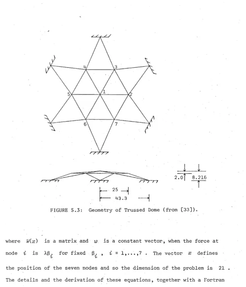
Problems of the form given in (1.1) often arise naturally in a form where it is necessary to find the value of x(t) for sufficient values of
t to define the solution (x(£),t) . The formulation describes how the state vector x(t) depends upon the control parameter t . There is a large literature on the theoretical and numerical analysis of such problems, much of it being in the theory of elasticity where x(t) represents the position of a structure and t represents a physical load. See for example [3], [6], [17], [33], [36], [38], [66], [69] and the references therein. Much of the analysis is involved with critical points on the solution
[x{t) ,t] of (1.1), i.e. points at which 9^//(x(t),t) is singular, and the
behaviour of the solution in the region of such critical points. As
mentioned above, some methods are described in Chapter 4 which are suitable for following solutions of (1.1). In Chapter 5 we develop these methods for the specific problem of following a solution through a certain kind of
critical point, known as a turning point. We suggest an improved technique, similar to the methods suggested by Riks [66] and Menzel and Schwetlick [49]. Turning points represent the boundary between stability and instability of a system and, as such, are of special interest. For example, Simpson [69] gives a numerical method for finding such points. In Chapter 5 we also consider this problem and present some methods which are more efficient than Simpson's method. It happens that the derived methods are also useful for finding certain simple bifurcation points, which are another example of critical points. One of the methods provides information useful for finding points on a secondary solution which emanates from a simple bifurcation point [37], [64].
C H A P T E R 2
C O N T I N U A T I O N W IT H S I N G L E - S T E P M E T H O D S
2.1.
I n t r o d u c t i o n
As a preliminary to the main results of this chapter we present, in section 2.2, a convergence result for the continuation methods introduced in
Yl 71
Chapter 1 for solving fix) - 0 , where f : D c: R -+ R . This result is not new in principle, but it specifies the type of conditions required on f
before convergence to x * can be guaranteed. It also indicates that the continuation method is not a panacea for problems with a poor starting guess, but that it can often widen the region of convergence. The theorem gives conditions on f and x for the solution of
(2.1.1) x(t) = -Jix) ^fix) , xiO) = x ,
to converge to x * .
and compare the methods suggested by the theory with some existing methods.
2.2. A C o n v e r g e n c e R e s u l t
In this section we consider the differential equation (2.1.1), where f i x ) is assumed to be continuously differentiable for all x F D . There are a great many theorems on the existence and uniqueness of solutions of
(2.1.1) (see e.g. [4], [8], [50], [53], [60], [72] and the references therein) but most are local in nature. Since the differential equation approach is concerned with wider convergence we present a theorem which is not local. The theorem is not new, having been proved with marginally greater assumptions on f by Gavurin [28], Deuflhard [23] and Ortega and Rheinboldt [53], but is given for clarity and as motivation for the overall approach. Its purpose is to characterise a region in which solutions of
(2.1.1) are guaranteed to converge to a zero of f . First we give some definitions.
D E F I N I T I O N
2.2.1. P a D is a region of stabilityof (2.1.1) if, for any x Q 6 P , the solution x i t ) of (2.1.1) is defined and unique for all t > 0 , x i t ) € P for all t > 0 and lim x i t ) = x* F P , where x* is af-Ko
zero of f .
Yl
For any nonsingular n x n matrix A define : D c R -* R by
cj)^(as) = f i x ) TATA f i x )
and, for any a > 0 , define -^^A) by
P (A) = {as I i ( D, d).(as) < a} .
a 1 1 A J
P (A) is a level set of A .(as) , (see [23], [53]). Let
a A
L = {x I as F D, Det(j(x)} = 0} . Then, for some a > 0 and P*(j4) , a path
A : P*(A) n L and _P^(A) n 9P are empty, P^(A) is bounded.
Under these conditions P*(A) is compact and contains one and only one
zero of f .
THEOREM 2.2.1.
Assume f : Dc
Rn-*
pn is continuously differentiableon D and a > 0 is such that condition A holds. If, in addition,
J(x) ^f(x) is Lipschitz continuous on Int(P*(A)) then Int(P*(A)) is a
region of stability of (2 .1 .1).
Proof. Standard theorems on ordinary differential equations (e.g. [32, Chapter 1]) show that, for any E Int(P*(A)) , there exists a T > 0
such that (2.1.1) has a solution which is unique in Int(P*(A)) for each
t € [0,T) . Also, if the maximal such T is not 00 and
{x{t) I 0 < t < t} has limit point x , then x € 9P*(A) .
I t T ot
When the solution x(t) of (2.1.1) exists it satisfies
(2.2.1) f(a:(t)) = e_tf(^0) = e~±f0 >
say, because (2 .1 .1) is equivalent to the initial value problem
df/dt - -/,/( 0) = f0 . Thus
$4 (*(£)) = e”2t^ ( Xq) > t * [0,T) , and so cf)^(a;(t)) is a decreasing function of t . Thus
*4 (*T) = Tim ^(a(t)) < a .
t->
T-Now suppose, if possible, that x^ £ 9P*(A) . Since P^(i4) is closed
and P*(A) n 9 D is empty there exists an £ > 0 such that S'(a: ,e) c D and
Pfa^jo) n {P^(A)\P^(A)} is empty, where ,S(a:,e) is the open ball with
centre x and radius £ . Let e. = £/i , then because x € 9P*(A) , for
l i m y . - x a n d , b y c o n t i n u i t y o f (f) ( x) , l im (J) ( y . ) = (p (x ) > a , w h ic h
t-x» t-x»
i s a c o n t r a d i c t i o n . Thus (: I n t ( p * ( A ) ) and i t f o l l o w s t h a t T = 00 , so
x ( t) i s d e f i n e d a n d x ( t ) € I n t ( P * ( d ) ) f o r a l l £ > 0 . A l s o , fro m
( 2 . 2 . 1 ) , i f x^ i s a l i m i t p o i n t o f ( x ( t ) } , t h e n f ( x m) = 0 . S i n c e a
z e r o o f / i s u n i q u e i n P*( A) i t f o l l o w s t h a t x = x* - l i m x ( t ) . T h i s
a °° oo
c o m p l e t e s t h e p r o o f . □
We n o t e t h a t a s u f f i c i e n t c o n d i t i o n f o r J ( x ) ^ f ( x ) t o b e L i p s c h i t z c o n t i n u o u s on I n t ( P ^ ( d ) ) i s t h a t , i n a d d i t i o n t o c o n d i t i o n A , J ( x ) be
L i p s c h i t z c o n t i n u o u s on I n t ( P ^ ( i 4 ) ) . T h i s f o l l o w s from t h e f a c t t h a t
||j ( i c ) ^|| and ||/(^c)|| a r e b o u n d e d on P*( A) and f ( x ) i s c o n t i n u o u s l y
d i f f e r e n t i a b l e ( a n d h e n c e L i p s c h i t z c o n t i n u o u s ) on P*(A ) . a
W h i l s t Theorem 2 . 2 . 1 i s n o t p r a c t i c a l l y u s e f u l , i t shows t h a t a r o u n d
e a c h z e r o a t w h ic h J ( x ) i s n o n s i n g u l a r t h e r e i s a r e g i o n o f s t a b i l i t y o f ( 2 . 1 . 1 ) . A l s o t h i s r e g i o n w i l l g e n e r a l l y b e l a r g e r t h a n t h a t p r e d i c t e d by
t h e l o c a l e x i s t e n c e t h e o r e m s . We e m p h a s i s e t h a t i f a : i s n o t i n s u c h a
r e g i o n t h e n c o n v e r g e n c e t o a r o o t i s u n p r e d i c t a b l e . We d i s c u s s t h i s c a s e
f u r t h e r i n C h a p t e r 6.
I n C h a p t e r s 1 , 2 a n d 3 we a ssu m e t h a t i s c o n t a i n e d i n a r e g i o n o f
s t a b i l i t y an d t h a t t h e s o l u t i o n t r a j e c t o r y o f ( 2 . 1 . 1 ) c o n v e r g e s t o a z e r o
x* . I f t h i s i s t h e c a s e t h e n , by f o l l o w i n g t h e t r a j e c t o r y c l o s e l y e n o u g h ,
we c a n g u a r a n t e e c o n v e r g e n c e t o x* . F o r t h i s p u r p o s e s e v e r a l o f t h e
s t a n d a r d m e th o d s f o r s o l v i n g i n i t i a l v a l u e p r o b l e m s may b e e m p lo y e d a n d , f o r
s u f f i c i e n t l y s m a l l s t e p s , c o n v e r g e n c e t o x* i s c e r t a i n . I n p r a c t i c e h o w e v e r , we w o u ld l i k e t o t a k e l a r g e s t e p s . F a r fro m t h e z e r o t h i s e n t a i l s
u s i n g a s o p h i s t i c a t e d s t e p s i z e e s t i m a t o r w h ic h w i l l a d a p t t h e s t e p
consistent with sufficient accuracy. Obviously the lower the accuracy the less work will be involved but the higher the probability of leaving the correct trajectory and diverging or finding the wrong solution.
Close to the solution, however, we can make use of the special characteristics of the problem to give rapid final convergence, using methods which are also suitable for following the trajectory far from the solution. In this and the following chapter we consider single and multistep methods, traditionally used for the standard initial value problem, which are adapted to give rapid convergence close to the zero x* .
2.3. General Theory
In this section we give some general results on iterative processes of the form
(2.3.1) ~ , i - 0,1,... ,
Yl Yl
where G :D x c: R * R -> R , and in the following sections we apply
these results to particular iterations. We use the results of Ostrowski [58] and Ortega and Rockoff [54] on processes of the form x^+^_ = >
G : D c Rn Rn , and generalise the existing theory to include the extra variable. We quote the following definitions which can be found in [53], except that here suitable modification has been made to allow for the slight generalisation.
Let C(1,x*) denote the set of all sequences generated by an iterative
limsup \\xh~x*\\^^ , if p = 1 , -R lx. } = •
P k 1
.
,limsup ^
k
9 if p > 1 .
The R-convergence factor of I at a;* is defined by R
= sup{i? {arfe} |
6 5(1,**)}
and the quantity0R (
I,**)
-•
is called the R-order of
I
at x* . We say that the convergence ofI
at x* is superlinear if R (I,x*) = 0 and linear if 0 < 5^(1,**) < 1 .the iterative process (2.3.1) if there exists an open neighbourhood S of
x* and a set I , called the h-domain of
I
, such that S cz D , I cand converges to x* . Also we say that x* is a fixed point of the iteration (2.3.1) if x* = G(x*,h) for all h € D« .
h
Finally, we say that G(x,h) is uniformly differentiable with respect to x at z € D on I c if, for each M l , G(x,h) is Frechet
differentiable with respect to x at z and if, for any e > 0 , there exists a 6 > 0 , independent of h , such that 5(2,6) c D and
for all x € 5(2,6) and for all h £ I .
We can now give conditions on G(x,h) which are sufficient for x* to be a point of attraction of (2.3.1). In this chapter and the next, if A
is a square matrix, q(d) will denote the spectral radius of A .
THEOREM 2.3.1.
Suppose that G :D xc
Rn x r -* Rn has a fixedand for any x^ £ S and any {/k } c= d the sequence \x^\ remains in D
point x* € Int(Z?) . Let' I c l be such that q(3 G(x* 9h)) S a < 1 for CL n
all h £ 1^ and suppose that G(x ,h) is uniformly differentiable with
respect to x at x* on I . Then3 if I i s non empty3 x* is a point
of attraction of iteration (2.3.1) with h-domain I .
Proof. The proof is almost identical to that given for the Generalised
Ostrowski Theorem in [53] and so is omitted. □
Theorem 2.3.1 is rather more general than we require and so we present
a corollary which is more suitable for our purposes.
COROLLARY 2 . 3 . 1
. Suppose G:
D xc
Rnx
r -y pn has a fixed pointx* 6 Int(Z?) . Suppose also that % G(x9h) and d^G(x,h) are Lipschitz
continuous on S x I where S is an open convex neighbourhood of x* and
I is an interval such that rif3 G(x*,h)) 5 a < 1 for all h € I . If
a K x J a
I' is nonempty then x* is a point of attraction of iteration (2.3.1) with
h-domain I
Proof.
It follows from the Lipschitz continuity of 3 G(x,h) and3yGixJa) and from [53, Theorem 3.2.5] that, for all ix,h) ( 5 x , there
exists a constant K such that
||G(a;,h)-G(x* 9h)- d^Gix*,h)(x-x*)\\ < X||x-x*|
This result is immediate if we assume that
= INI t I ot I ,
however the result follows anyway if we use the equivalence of norms. Now,
given e > 0 , if K6 < e then, for all h € I ,
a
\\Gix ,h)-Gix* ,h)-d^G(x* 9h) (x-x*) || < e||:c-a:*|
respect to
x
atx*
on. . The result now follows from Theorem 2.3.1. □Corollary'2.3.1 gives sufficient conditions for local convergence of the iterative process (2.3.1) but gives no information on the rate of convergence. For this we require conditions on
[h^\ .
We begin byderiving a result on the assumption that lim
h
. exists.T H E O R E M 2 . 3 . 2 . Suppose G : D x c Rn x r -> pn has a fixed point
x* e Int(£>) 9 and that d^Gix,h) and d^Gix,h) are Lipsohitz continuous
in a neighbourhood of ix* ,h*) , where lim h. = h* E Int [D-^] . If
i-x»
a = r\ [d^G(x* ,h*) J < 1 then x* is a point of attraction of the iterative
process T given by (2.3.1). Moreover
i? (I ,x*) - a
and if a > 0 then O^il ,x*) = 1 .
P r o o f . Define uix,h) by
(2.3.2) Gix,h) = G(x* ,h) + d^G(x* ,h)ix-x*) + uix,h) .
Then, as in the proof of Corollary 2.3.1, there exist positive constants
K , 6 and 6^ such that
(2.3.3) \\uix,h)\\ 5
for all x E Six*,6 ) , h E (/z*-62 , say. Furthermore, from the
Lipschitz continuity of d^Gix,h) , with Dih) defined by
(2.3.4) D(h) = 9 Gix*,h) - 3 Gix*,h*) ,
there is a constant > 0 such that
(2.3.5) \\D(.h)\\ S K 2 \h-h*\
for all /z E J 2 .
G(x,7z)
- x* -
G(x*9h)
+
9 G(x* 9h)(x-x*)
+ w(x,/z)
-
x*
and so(2.3.6)
G(x9h) -
x*
=
D(h)(x-x*)
+ 9
G(x*9h*)
(x-x*) +
u(x,h)
.
cc
Yl
For arbitrary
e >
0 there exists a norm onR
such that||9 G(a:*,7z*)|| <
a+ £
[53, Theorem 2.2.8] and in this norm, if
6
satisfies<
£ it followsfrom (2.3.6) that, for any
h
€
»\\G(x,h)-x*\\
5 (#
21
h-h*
|
+a+2e) ||x-x*||
for all
x
€
S(x*
,6)
. Also since {/r.} converges to A* , there is an -7 such that 1 /z.-h*
I 5 £ for alli >
.
If £ is chosen so thate/#2 < ^2 » then /k
6
J2
for alli
> , and if x^. € £(x*,6) , itfollows that
lkt+r**H ^ (a+3e) Ux^-x^ll .
Since a < 1 and £ may be chosen so that a + 3e < 1 , it follows from [53, Theorem 10.1.2] that i?^(I,x*) < a . If a = 0 this completes the proof.
From (2.3.6) we also have, for all
(x9h)
€ jS(x*,6) x s ||£(x,?2
)-6(x*,h*)-d G(x* ,h*)(x-x*)\\
=
\\D(h)(x-x*)+u(x9h)\\
cc
5 (^
21
h-h*I
+£.J|x-x*||) ||x-x*|| .
Now if < £/2 and
e/2
5
we have(2.3.7)
\\G(x9h)-G(x*
,h*)-d^G(x* ,h*)(x-x*)
|| < e||x-x*||for all x € <S(x*,
6) and for all
h
€
•
The remainder of the proof is almost identical to the proof of the Linear Convergence Theorem given in [53] with (2.3.7) replacing equation (10.1.7) in [53] and 9^G(x*,h*)
replacing G f(x*) . □faster convergence in the, case when r\[d^G(x* ^h*)] = 0 . For this case we
require further knowledge of the sequence \Pj\ •
T H E O R E M 2.3.3.
Suppose G:
Dx
c:
Rnx
r-*
Rn satisfies theconditions of Theorem 2.3.2 and that
r i , 7 z * ) )
= 0.
Then (x*,h*) isa point of attraction of the iterative process
I
given by (2.3.1) and R (I,x*) = 0 . If3 in addition,
{h c o n v e r g e s to h* with R-orderr > 1 then 0^(1 ,x*) > min( 2 where k is the unique integer such
that
3
=
0 and3 £(o;*,/z*)k ^ ^ 0 .
x
5
x 9Proof.
Theorem 2.3.2 shows that x* is a point of attraction ofI
and that i? (I,o;*) = 0 so we may assume that {o n} converges to 0;* .
Let A - 3^£(o;*,/2*) . Then q(/l) = 0 and there is an integer k < n
1 1c
such that A ^ 0 and A = 0 . With the definition of u(x,h) and
D(h) given in (2.3.2) and (2.3.4), let D^ = T>{hP\ and u^ = u[x^,h^) .
Then, if we write e^ = x^- x* it follows from (2.3.6) that
1+1 D .e.
+
and, by induction, for j > 0 ,
(2.3.8) e. = Ap e - . + D. .e. .+ ...+ j4Z). 0e . 0 + D. e.
^ t-2 ^-2 ^-l ^-l
,j-l
+ A w . . + . . . + 0 + 12. , .
t-j t-2 ^-l
Since {x^\ and {^} converge to 0;* and /z* respectively, it follows 2 from (2.3.3) and (2.3.5) that, for all sufficiently large i
,
\\ud\<
K^e .and ||z?
II
< 5 w^ere = |?k -7z*| . Since A - 0 , it now followsK'l S
Kl [ ^ ei - /
+
+
21
'2 + l|ei-l112.
where y = ||A|| .
+ ♦ . . . + Y ll« < _
2
l|ei_2
+ ll« i _1
l|ei _ iSince \xj] converges to x* , it follows that there exists an £^ > 0 and constants B , B^ such that, for each £ > £ ,
Ikjll 5 B i ^ e i-k^ + B 2^ei-k^£i-k’ R e p l a c i n g £ b y k £ a n d w r i t i n g ou = ^ 1 lle ^ l l a n d = ^ 2 ^ k i w e ^ a v e
(2.3.9) a . < a . , + a . , $. , ,2 ^ ^ - l ^ - l ^ - l for all sufficiently large £ .
We now require the result that, if 1 < p < min(2,r^) , then there exists a constant c > 0 and a j > 0 such that
(2.3.10)
£ „ -ep a. 5 e r
for all £ > j . To prove this, suppose that s satisfies p < s < min(2,r^)
k
r ,
. Then, because {(Li converges to zero with Z?-order
(2.3.11)
£ g. 5 e-S
for all £ sufficiently large. Let c be some constant, yet to be determined, then because p < s , it follows that, for £ sufficiently large,
(2.3.12) e -s ^ < e r-op
Also, since {ou} converges to zero and p < 2 ,
(2.3.13) a. 5 e-1112^ 2-?)
(2.3.13) are all satisfied for all £ > j and suppose that ou 5 e-ep for
some
• • •
£ > j . Then, from (2.3.9), - e ^ + e S e and, from
_ 2
i
_
£+1(2.3.12), a. _ < 2e . We wish to deduce that a. , < e
’ ^+l ^+l and
-2e ^ -c ^+1
this will be so if 2e < e . Some simple algebra shows this to
be the case if
(2.3.14)
a
>and a suitable choice for o is
o
-In 2
p^(2-p)
In 2
p d (2-p)
for then (2.3.14) is satisfied for each £ > j . Now, by choice of c , J
a . < e J
and we have shown that, assuming (2.3.10) for some £ > g , then
(2.3.10) follows with £ replaced by £ + 1 . So, by induction, (2.3.10)
is true for all £ > j as we required.
It now follows from (2.3.10) that the P-order of the sequence {ol.}
is at least p . Since ou = ||e^|| and p is arbitrarily close to
min(2,r^) , it follows that 0 (I ,#*) > m i n ^ ^ ^ p j .
2.4. Runge-Kutta Methods
Consider the general class of explicit Runge-Kutta methods for solving
the differential equation
(2.4.1)
x(t) = q(x)
, x(0) = ,given by
v
(2.4.2a)
x
,- x
+h
Y a.k.[x
,7z 1 ,m
- 0,1,... ,m+1
m
m
.%where
x
is an approximation tox[h.
++
... +h
m
^ 0 1m
-11 J=1
and is the step length. A discussion of stability for this method is
usually based upon consideration of the linear differential equation
(2.4.3)
x(t)
=Ax
, jc(0) =xQ
,where
A
is a fixed matrix whose eigenvalues have negative real part. The true solution of (2.4.3) isx[t+h^]
= exp(h A]x(t)
whereas the solution given by (2.4.2) is
where
p(z)
is a polynomial of degreer
whose coefficients depend upon choice of the a's and ß's in (2.4.2). The usual practice is to choosethese parameters so that
p(z
) is a good approximation to exp(s) . We note that, since the true solution of (2.4.3) is decreasing, a requirementon the step length
h
is that the conditionbe satisfied so that the iterates in (2.4.4) also decrease. However, in the
nonlinear case, (2.4.5) is of little practical use in controlling the
stepsize.
In this section we consider (2.4.2) not only as a means of approximating
the solution of (2.1.1) but also as a one-step method for finding a zero of
f
. For the former the theory is well known [34] and for the latter we use the results of section 2.3. In this case we have(2.4.4)
m
(2.4.5)
m -
0,1,..x
'm+1
m = 0,1,..r
(2.4.6)
G(x,h)
=x
+h
X ot.k.(x,h)
i
=1 'Z''
l
and
k^ix^h)
is given in (2.4.2b) fori -
l,...,r . We apply this process to the case whenqix)
is given by(2.4.7)
qix) = -Jix) ^f(x)
.Then, if J represents the unit matrix,
r
3
G(x9h) = I + h Y a.d k.ix,h)
.x
.w , ^x
^^=l
If
x*
is a zero offix)
thenx*
is a fixed point of (2.4.2) and also, from (2.4.7), we haveq ’ix*)
=-I
,where the prime denotes differentiation with respect to
x
. It then follows by some simple algebra that(2.4.8) 3
^G(x*,h) = p(-h)I
where
piz
) is the same polynomial as appeared in (2.4.4). Rather than proving this result here, for the sake of continuity we present it in the appendix to this chapter as Theorem 2.4.1. It now follows from Corollary 2.3.1 that a sufficient condition forx*
to be a point of attraction of (2.4.2) is that, for some a < 1 ,(2.4.9) n ( p ( - k j h = 2 a , m = 1,2,... ,
which, unlike (2.4.5), provides an
explicit
bound on each for ultimate convergence tox*
. We note that the region of the complex plane defined byIp i z)I < 1
the iterative process can. give superlinear convergence to x* only if h* satisfies
(2.4.10) *
p i - h *
) = 0 .Therefore, when
fix)
is three times continuously differentiable it follows from Theorem 2.3.3 that if j/j } converges to h* with R-order > 2 , thenthe iterative process (2.4.2) has i?-order at least 2 .
In the application of (2.4.2) it is of benefit to choose the parameters so that the resulting method will follow the solution of (2.1.1) well enough to inhibit divergence but will also provide a fast rate of final convergence to
x*
. This means choosing a method which allowsh*
to be chosen so that (2.4.10) is satisfied. We note here that for the well-known 4th-order Runge-Kutta processpiz)
is defined by2 3 4
p(z)
= 1 + 2+ §r+ fr + fr
and
p i - z
) has no real root. Thus no choice ofh*
can furnish superlinear convergence. Also Heun's predictor-corrector method [34] may be writtenq [x
)
+q [x +h q [x
11
mJ ^ k m rrr K mJ This is of the class (2.4.2) and has
piz)
defined by2
piz)
= 1 +
z
+ ~ .
This is simply a Runge-Kutta method of order 2 and again
pi-z)
has noreal root, so no choice of
h*
can give superlinear convergence tox*
.
In attempting to solve (2.1.1), Boggs [9] used this method as an explicit approximation to the trapezoidal rule.We note that for these two methods we can use Theorem 2.3.2 to show that
t Note that "order" is a term related to the accuracy of single and multi-step methods in following the trajectory
xit)
(see [34] and the definition of //-order in section 4.2), while the term "//-order" is related to the speed of convergence of a sequence to its limit (see section 3.2 and [53]). (2.4.11) x -i — x +O ß ( I , x * ) = 1
and
= \p(.-h*)\ .
So assuming (2.4.9) is satisfied, convergence is at best linear and the
(2.4.9), then the method will not generally converge.
Boggs [9] in his paper suggested there is a difficulty of stiffness involved in integrating (2.1.1). Stiffness is a problem which occurs when solving the differential equation
when q'(x) has eigenvalues with widely separated negative real parts. Their numerical solution requires the generation of special methods which are ^-stable [18] or at least stiffly stable (see [29] for a full
description of these concepts). One characteristic of an unsuitable method applied to a stiff system of differential equations is for the iterates to oscillate about the true solution and possibly diverge. In our problem, however, q ’(x*) = -I and so, close to x* at least, (2.1.1) is most certainly not a stiff system. The symptoms of instability which Boggs ascribes to stiffness appear identical to the behaviour observed if the
sequence {?2^} contravenes (2.4.9). If we attempt to solve the differential
equation (2.1.1), the standard methods tend to allow {h^ } to increase as the
zero is approached, since the rate of change in direction of the solution trajectory is decreasing. If this happens then oscillation and divergence of the sequence {ar.} maY occur if hm becomes too large, as would be the
case, for example, when using Newton’s method with a steplength greater than 2 . When the step is suitably controlled no problems of instability occur fastest convergence is achieved by choosing h* to minimise
For Heun’s method this is h* = 1.0 when i?^(I,a:*) = % and then
and, indeed, as long as h satisfies (2.4.9) for each m , close to the
0 m
zero the problem is extremely stable, simply because any zero of f is an asymptotically stable node of the autonomous differential equation (2.1.1) [45].
The foregoing theory shows that any method giving a polynomial p ( z) such that p(-h) has a positive real root will be effective for producing rapid final convergence if {/z^} is suitably chosen. For example, we
consider briefly Runge-Kutta methods of orders one, three and five. The simplest first-order method is Euler’s method. In this case
p(z) is given by
p(z) = 1 + z
and, from (2.4.9), we see that x* is a point of attraction with /z-domain [6,2-6] , for 6 arbitrarily small, i.e. local convergence is guaranteed if 0 < 6 < h 5 2-6 for each m . Also, from (2.4.10) and Theorem 2.3.3, the
m
R-order of convergence to x* can be > 2 if {/z^} converges to 1 with
Z?-order at least 2 . This is essentially Newton’s method.
There is a class of third-order Runge-Kutta methods and, for each,
p(z) is defined by
2 3
/ \ z z
p{z) - 1 + 2 + — + — .
Now Ip(—h)I < 1 if and only if 0 < h < , where h^= 2.5127 ... , and
so, from (2.4.9), each of these third-order methods converges locally to x*
with /z-domain [6,/z^-6] , for arbitrarily small 6 . Also, the i?-order of
convergence to x* can be two if { ^ } converges sufficiently fast to
h - 1.596 ... , where is the only real root of p(-z) .
h
= 5.6039 ... , and sox *
is a point of attraction with ^-domainu
[6
,h
-6]] , for 6 arbitrarily small. Again, convergence tox*
hasR
-order 2 if converges sufficiently fast toh.* -
2.6299 ... ,where
h*
is a real root ofp(-z
) .The conclusion of this section is that there exist single-step methods which can follow the solution trajectory of (2.1.1) sufficiently accurately and which, by suitable control of the step length, can furnish rapid
convergence to
x*
. In section 2.5 numerical details are given for a third-order method which adapts the step length until it reaches a maximum ofh
= 1.596 ... , after which it is not allowed to increase further.r
For completeness, we note here that the principles described in this chapter can be extended to implicit Runge-Kutta methods and to the
predictor-corrector methods based on them. As an example we describe Heun’s approximation to the trapezium rule with an extra correction, since this method was used by Boggs in [9]. Using standard notation (see [9], [29]), Heun’s method, given in (2.4.11), can be considered as a predictor-
corrector method of the form
P : p = x + h q ,
r m m rrrm
E : q = q[p ) ,
h
C :
xm+lxm ' - f
E :
C :
« m1 =
+ T
’
E
:
Vl =
»
h
C : re .. = x +
~ [a +q
, OT+1m
2 L^m ^m+lJ which can be written in the iterative form(2.4.12a)
y
, =x
+ -771
m
2(2.4.12b) a; = a;
m+1 m +
•
— \q [y
2 [jyiJmJ
)+ q x + -?• {q{u )+q{x +h q[y ))}
H
[m
2 1 ^KSJmJ H y m m yjmjJ
Definez^
,m -
0,1,2,..., and 3* bym
_[ i _ - a LetI
denote the iterative process (2.4.12), then Is _ =
G[z ,h )
,m+1
y m
which is of the form (2.3.1). In the case that
q(x)
fix*) =
0 , some simple algebra shows that 3G(z*,h)
A ,A which satisfy
can be written as
=
-J(x) ^f(x)
and has two eigenvaluesA 1 + X 2 =
f
^
h~ + 1 = e ( h )say. Since
0(h)
has no real roots and the minimum value0(h)
is 2/3 , it follows thatn(3
G(z*,h))
> 1/3for all
h
. Theorem 2.3.2 shows that, like H e u n ’s method, convergence of this process tox*
is at best linear and Z?^(I,x*) > 1/3 .2 . 5 .
N u m e r i c a l R e s u l t s
We begin by making some general comments on the effectiveness of
necessary to assume that is in a stability region of a zero
x*
, for if this is not'so then convergence is not guaranteed, there are applications where the approach will be effective. For example, where the usual methods diverge or continually converge to a zero which is known but where the user requires to find a different zero, which he knows to exist, and has asuitable starting point. However, one should realize that, whilst the number of evaluations required to follow the trajectory sufficiently accurately may seem reasonable to one used to solving ordinary differential equations, it may seem surprisingly large to one used to solving nonlinear equations.
Following the trajectory
x(t)
is usually a simple matter ifh
can be chosen sufficiently small, but in practice an important part of solving (2.1.1) is in the step length control. Far from a zero off
all of the usual problems of step control occur and great care is required to maintain accuracy. Close to a zero off
this is not the case so long ash
is controlled in a way which will guarantee convergence, i.e. so long ash
satisfies (2.4.9) for each
m .
Asx*
is approached we are less interested in accuracy in following the trajectory than in convergence tox*
andindeed, if we are to achieve fast ultimate convergence to
x*
, we must relax our preoccupation with accurate representation ofx(t)
whichconverges to
x*
only linearly (see (2.2.1)). In the examples that follow we are interested only in demonstrating ways of achieving faster final convergence and so we look only at cases when is fairly close tox* .
In this case the criterion for varying
h
can be simpler than would be necessary in the general case.The basic technique is based upon the fact that the solution of (2.1.1) satisfies
m
/ ( ? ( £ ) ) = e
tfixQ)
•Z . = T -
f
A
A
'Then any point a: , on x(t) , satisfies
ZQf(x) = 0 .
Suppose is our current approximation to a;* , then the solution of
a;(t) = -J(x) ^f(x) , x(0) = x. ,
converges to x* (under the conditions of Theorem 2.2.1) and ||Z^/h+^||
gives a measure of the deviation of from this trajectory. On this
basis a suitable step change criterion was found to be = min {h* ,cx/k )
where oi is given by
'2 if 0 < 6 5 e1 ,
(2.5.1) a = ■1 if e1 < 6 5 e2 , 0.5 if
E2 " 6 S £3 »
6 = UZ^/h || an<3 is the step size necessary for the fastest convergence for the method. In addition, the point was rejected and the step
repeated with half the step length if either 6 > or
Det (j ? Det; (<7 C^q) ) > in which case the iterates had crossed a region
of singularity of the Jacobian.
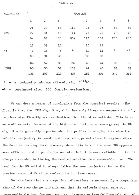
Various methods were tested on a variety of problems and the results of some of these tests are tabulated below. As an example of a method with rapid final convergence we chose a third-order Runge-Kutta method (RK3) for which h* - = 1.596... . For comparison we tried Heun's method (HEUN)
iteration consists of integrating
(2.5.2) , x(t) - -J(x) 1/(yr.) , x(0) =
Ji ’
giving a sequence {y . .} , J - 1 , such that y. . is an
t , j t t, j
J-l
approximation to .) , where . = £ /r. ^ and ^ = 1 . Then /c=l "£•
~ yi N . ~ ^i+1 i * ^ is proved by Kleinmichel [41] and Bittner [7]
that, under general conditions, if the method uses step size h* = 1 then the sequence \x^\ converges to x* with i?-order 4 . Despite this high
rate of convergence, the greater demand on accuracy required in following the solution trajectory of (2.5.2) when x^ is not close to x* causes the
algorithm to be less effective than those described in this chapter.
For a fair comparison of methods we used a similar step control to that described above. Since the solution of
x(t) = -J(x)~1f[yi'.) , x(0) = y ^ ,
does not generally converge to x* and may, in practice, cross a region of singularity of J(x) , it is necessary that each y^. be close to the
solution trajectory of (2.5.2). In this case, therefore, the most suitable criterion is that h. . = m i n[ah. . ,1-t. . ) where a is given by
t,J+l tsjtl
(2.5.1) and 6 = \\Z^f[y^ j+q) II • Also we took
h. = min(l,2 max [h. ,/z. )) . The conditions for rejecting a step 5 JL Is 5 IV ^ Is $ I V ^ i
were the same as before.
In each algorithm = 0*5 , = 0*25 and £^ = 0.05 were found to
x
0 *
1. A function found in Boggs [9];
7T
C O S — X
2 »
with initial guess x = (1,0) . The correct solution is x * = (0,1) .
2. Problem 1 with initial guess (-1,-1) . The correct solution is
(0,1) and the solution trajectory passes close to a region where J ( x ) is singular.
3. A function found in Broyden [15];
with initial guess (-1.2,1.0) . The correct solution is (1,1) and this
problem can be considered fairly difficult since the solution trajectory is
always close to the region where J ( x ) is singular (see [11]). 5. A function found in Branin [11];
sin (x^Xy) - £ 2/(4tt) - x ± /2 , 2 x
f 2 - (i-1/(4tt)) (e 1-e) + ea^/ir - 2 e x ± ,
with initial guess (.6,3.) . The correct solution is ( % ,t t) . 4. The gradient of Rosenbrock's function;
= 400 x x + 2(x1-l) ,
f - 2 sin (2ttx /5) sin (2tt:c3/5) - x2 ,
f 2 - 2.5 - + 0.1 i 2 sin(27T^3) - ,
/ 3 = 1 + 0.1 x 2 sin(2TTo:1) - x3 ,
with initial guess (0,0,0) . The correct solution is (1.5,1.809 ...,1.0) .