Quantities from Different Levels of Data
The Harvard community has made this
article openly available.
Please share
how
this access benefits you. Your story matters
Citation
Alt, James E., Gary King, and Curtis Signorino. 2001. Aggregation
among binary, count and duration models: Estimating the same
quantities from different levels of data. Political Analysis 9(1): 21-44.
Published Version
http://pan.oxfordjournals.org/
Citable link
http://nrs.harvard.edu/urn-3:HUL.InstRepos:4125133
Terms of Use
This article was downloaded from Harvard University’s DASH
repository, and is made available under the terms and conditions
applicable to Other Posted Material, as set forth at
http://
Aggregation Among Binary, Count,
and Duration Models: Estimating the
Same Quantities from Different
Levels of Data
James E. Alt
Department of Government, Harvard University e-mail: [email protected]
Gary King
Department of Government, Harvard University and World Health Organization, Cambridge, MA 02138
e-mail: [email protected] WWW: http://GKing.Harvard.Edu
Curtis S. Signorino
Department of Political Science, University of Rochester, Rochester, NY 14627
e-mail: [email protected]
Binary, count, and duration data all code discrete events occurring at points in time. Al-though a single data generation process can produce all of these three data types, the statistical literature is not very helpful in providing methods to estimate parameters of the same process from each. In fact, only a single theoretical process exists for which known statistical methods can estimate the same parameters—and it is generally used only for count and duration data. The result is that seemingly trivial decisions about which level of data to use can have important consequences for substantive interpretations. We de-scribe the theoretical event process for which results exist, based on time independence. We also derive a set of models for a time-dependent process and compare their predic-tions to those of a commonly used model. Any hope of understanding and avoiding the more serious problems of aggregation bias in events data is contingent on first deriving a much wider arsenal of statistical models and theoretical processes that are not con-strained by the particular forms of data that happen to be available. We discuss these issues and suggest an agenda for political methodologists interested in this very large class of aggregation problems.
Authors’ note:Our thanks go to Mike Gilligan for research assistance, Henry Bienen, Andrew Gelman, and Nicholas van de Walle for their comments on early versions of the manuscript, and the National Science Foundation (Grants SES-9817947, SBR-9729884, SBR-9321212, SBR-9223638, and SES-8909201), the Centers for Disease Control and Prevention (Division of Diabetes Translation), the National Institutes of Aging, the World Health Organization, and the Peter D. Watson Center for Conflict and Cooperation for research support.
Copyright 2001 by the Society for Political Methodology
1 Introduction
Data in many disciplines are often coded from specific events, and a well-developed methodological literature has emerged to deal with such data. In political science, and other fields, three important coding schemes have been used. The first,durations, measures the interval between events. The second,counts, measures the number of events that have occurred within “slices” of time. Finally,binarydata are often the finest-grained, resulting either when count time slices are reduced to such an extent that at most one event occurs in any observation or when count data is “censored” to zero and one.
Suppose we wish to explain the occurrence of some type of event. We could choose any level at which to measure the process if we collected the data ourselves, but one level is often the most convenient to code. Alternatively, as is so often the case, we might have obtained the data from someone else. Of course, it is not the arbitrary unit of analysis or form of aggregation which forms the focus of our inquiry; rather, we wish to explain what generates the events under study.We do not want the form in which the data happen to be collected to determine the substantive ideas which we can explore.Instead, we should identify what we believe the underlying data generating process to be and then use the appropriate statistical model for that process and for the given data to evaluate our substantive ideas. In one very special case, methodologists have shown that it is possible to specify a single theoretical model of what generates the events and to estimate its parameters regardless of the level at which the data are aggregated. But the events process literature does not include even one other set of models for which this is possible. If the one special case does not happen to be substantively plausible in a specific application, the researcher is stuck using incompar-able models and may have to settle for substantive conclusions that depend heavily on how the data happened to be collected.
Unfortunately, although perhaps reasonably from the perspective of individual resear-chers, the analysis of each type of data has proceeded without attention to how other researchers set up their models. For example, when confronted with binary data, most researchers automatically use a logit or probit model. Duration data are usually analyzed with models based on complications of the exponential (e.g., weibull, gamma, compound, competing risks, etc.). Scholars usually model count data with a poisson or compound-poisson model. Individually, these are each reasonable choices.
However, the statistical literature does not generally provide ways of comparing results across these different models. This should be quite frustrating to scholars, since binary, count, and duration data are all coded from precisely the same underlying events.1Applied researchers need not disagree over results that depend incorrectly on the unit of analysis chosen, especially if these disagreements could be resolved, or at least reduced, if these researchers could estimate models at any level of analysis. Our primary goal in this paper is to demonstrate how to compare the results obtained from binary, count, and duration models of the same underlying data generation process.
Relating techniques for modeling each sort of data requires understanding the roles of aggregation or disaggregation in statistical models for events processes. Different methods of data collection lead to testing different models, and some different sorts of information may be lost at each stage of aggregation. The statistical literatures bearing on events data have their own unique notation and specialized mathematical concepts—both of which do not exist in other areas of statistics that may be more familiar to political scientists. Thus,
1A similar point is made by Petersen (1991) about events data and by Freeman (1989) in the context of aggregation
in the sections below, we begin by introducing a notational scheme for the three types of data—binary, count, and duration.
We also examine two types of processes that might generate the various forms of data. The first, and the simpler, assumes independence of events and results in the familiar exponential model of event durations, the poisson model of counts, and a model for binary data that we develop here. The second data generation process applies to events that are time dependent. We derive statistical models for analyzing them. A key point throughout is that the theoretical data generation process is separate from the unit of analysis in which the data happen to be recorded. In theory, one can estimate the same parameters in all three types of data, although some forms of data provide more information about the quantities of interest.
This is more than just a theological point. We view this paper as part of a larger agenda to which we hope political methodologists will devote some of their attention. For simple linear models and continuous individual-level variables, scholars have identified the assumptions necessary to infer from aggregate data to individual-level relationships (for a review see Stoker 1993). Progress has also been made with the ecological inference problem, which involves filling in the cells of a set of cross-tabulations from the observed marginals in each (King 1997). Unfortunately, very little work has been done attempting to resolve aggregation problems for event processes and other types of sophisticated statistical models. A handful of articles have addressed components of the larger problem.2However, the broader subject
does not appear to have been addressed more generally.
To deal with aggregation bias appropriately in these models, two steps are necessary. First should come models, such as those provided in this paper, which at least under certain specific assumptions are able to estimate the same parameters no matter what level of analysis or type of aggregation produced the available data. Only by having at our disposal a set of models such as these for each theoretical process of interest will the field be able to move forward to the ultimate goal of resolving aggregation bias problems wherever they may occur. Developing models that can avoid aggregation bias in events process models, and in other areas, will require a second difficult set of developments. But these developments can only occur after, or at least concommitant with, the first. Thus, this paper is only directed toward the first step in this research program. To be successful, to produce truly practical results, political methodologists will need to work on each of these issues, and much remains to be done.
This paper does not review the extensive statistical literature on event models. This literature is quite rich and we touch on but a small portion of the parametric models for these data.3 We illustrate our theoretical results with simulated data by appeal to a
spe-cific empirical literature which motivated our substantive and methodological research in this area. The use of simulated data allows us to isolate the various types of error that might appear in real data—thus allowing us to focus solely on the theoretical is-sues presented in this paper. Most of the models introduced here aid our methodological purposes; more research will be necessary to determine to what data they would best be applied.
2For example, D’Agostino et al. (1990) analyze the relationship between pooled logistic regression and dependent
cox regression. Aalen (1992) studies the application of a compound poisson model to survival analysis. Dean and Balshaw (1997) examine efficiency issues in analyzing event counts versus event times.
3See Box-Steffensmeier and Jones (1997) for a very nice review of event history models in political science;
Section 2 introduces a general notational scheme and a running example used throughout this paper. In Section 3, we show how results may be compared across time-independent models, proceeding then in Section 4 to do the same for a set of time-dependent models. Section 5 concludes.
2 Transfers of Governmental Power as a Renewal Process
The general class of “counting” processes addressed in this paper fall under the rubric of
renewal processes. A renewal process is simply an event process where the arrival times (or durations) between events are independent and identically distributed, according to some arbitrary distribution (see, e.g., Ross 1993, p. 303). Many examples of renewal processes exist in the literature in political science, such as the occurrence of war or a coup. We use transfers of governmental power as our running example since this is one of the most active areas of substantive research in political science with all three types of data and the methodological questions presently at issue.4
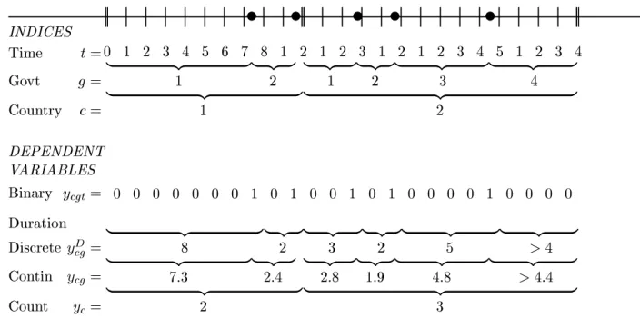
We begin by describing the data which constitute our information about transfers of governmental power. Figure 1 portrays the basic events and defines some symbols that will be helpful in discussing various models of these processes. A time line is the key part of this figure, with countries separated by double vertical lines and the five transfers of governmental power indicated by dots on the line. The time line is indexed bycfor country
Fig. 1 Units of analysis and types of dependent variables for transitions of power. Indices corre-sponding to time, government, and country units of analysis are denotedt,g, andc, respectively. Binary, duration, and count dependent variables are denotedycgt,ycg, andyc, respectively.
4The transfers—whether constitutional or nonconstitutional, democratic or nondemocratic, or electoral or
[image:5.612.119.471.361.536.2](c=1, . . . ,C),gfor a government within countryc(g =1, . . . ,Gc), andtfor a time unit (such as a month or year) within a governmentgand countryc(t =1, . . . ,Tcg). Thus, the time unit indextis incremented within governments and is restarted with each transfer of power.
This basic setup may be coded as binary, duration, or count data. We label a variable representing binary data asycgt, where
ycgt =
1 if a transfer of power occurs duringt
0 otherwise (1)
This coding was used by Londregan and Poole (1990), for example. It is the most disaggre-gated form of data usually used and enables one to model explicitly both the cross-national and time series processes underlying the data. The former is useful for comparative pur-poses, and the latter provides multiple instances to study within each country. However, some information is nevertheless lost in the coding process. In particular, in going from a representation like that in Fig. 1 toycgt, one loses the information about when a transfer of power occurs during the time unitt. Ift is a year or longer, this information loss can be substantial, adding considerable measurement error to the variable. On the other hand, ift
is as short as a day, the information lost may be nonexistent or irrelevant.
A list of all the durations between transfers of governmental power is a different way of coding these events. Duration data may be coded as a discrete or continuous variable. As a discrete variable, one merely counts the number of time units (e.g., months) between events. We denote this variableycgand calculate it as a deterministic function of the binary representation, simply summing over time within durations:5
ycg= Tcg
t=1
1=Tcg (2)
The only information lost by this coding of the transfers is the precision of when within each time unit a transition occurs. Thus, at worst, discrete durations include some grouping error.
One can also code a continuous version of this variable, which is the exact length of time that passes between transfers of governmental power. Virtually all durations used in social science data analyses are really discrete, since we never code more precisely than days and rarely finer than months. In practice, the difference in the models designed especially for the discrete and continuous versions of these variables does not produce empirical results that differ sufficiently to justify presenting both versions. We therefore focus on the discrete versions.
Finally, these data are sometimes coded as counts—the number of government transfers that occur in each country or in each country during some fixed period of time. Counts are deterministic versions of the binary and duration data. We denote counts of transfersycand
5While the individual binary-level time period may be of any length—as long as only one event may occur in
calculate them as follows:
yc= Gc
g=1
Tcg
t=1
ycgt = Gc
g=1
1=Gc (3)
This format may be useful for the study of variation across countries in the stability of their governments. Considerable information is lost in the count version of these data, including any variation in the duration of governments over time and any time series process in that variation. However, aggregating to the country level in this way also cancels out a lot of measurement error.
To get an intuitive sense of this problem, suppose we make one mistake by omitting one transfer of governmental power. The binary variable will have a mistake in one observation (where the zero in that cell should be a one). The duration coding will have one fewer observation, and the observation just before the transfer that was omitted will be longer than it should be. Each of these can cause problems with any statistical analysis. However, in the count variable, missing only one transfer may not have much of an effect, especially if a country has a large number of transfers. Of course, the critical point here is only that coding errors affect the different levels of aggregation in different ways; depending on the exact process generating the underlying events, measurement error can have different effects at the different levels of statistical models.
We have addressed the dependent variables for all three types of data, but what of the independent variables? For example, it is plausible that a theory of governmental transition of power would relate government transition to specific characteristics of each state, of each government, and of other factors that vary more frequently over time (e.g., inflation or unemployment). Here, we denote the resolution of the explanatory variables using the same notation as for the dependent variables:xcgt for time-varying data,xcgfor data that varies between governments but not over the binary-level time periods, andxcfor data that varies between countries but not over governments or binary-level time periods.6It is the
parameter estimates for these explanatory variables that we seek to compare across the three models.In the rest of this paper, we show how to estimate the same parameters using the three forms of the transfer of power data.
3 Analyzing Time-Independent Renewal Processes
The simplest and most commonly known renewal process is the poisson process—where the interarrival times are independent and identically exponentially distributed. Here, after one takes into account the explanatory variables, transfers of governmental power are “Markov independent” or “memoryless”—i.e., the probability of a transition of power in any period after timetis always the same, conditional on everything that happens up to timet, but not ont itself. (We also call this “conditional independence” to emphasize that this statement is only true after taking into account the effects of the explanatory variables.)
Violations of Markov independence would occur if, after taking into account the ex-planatory variables, the probability of a transfer of power increased over time. For example, Bienen and van de Walle (1991) propose a model inconsistent with this assumption since
6By definition,xcgtmay include government and country-varying data andxcgmay include country-varying data.
they believe that after a leader has been in office for several years, the probability that he or she will be removed drops. Markov independence is therefore a key substantive assumption that should not be taken lightly. We use it as a starting point here because it is so transparent and because it is the basis for (or a special case of) a number of other more complicated models. Section 4 provides a generalization that allows us to drop the assumption of Markov independence.
3.1 Duration Data
We start with the duration model for two reasons. First and foremost, renewal processes are often defined in terms of (or derived from) the assumed distribution of interarrival times. Second, discussion of the hazard rate highlights the time-independent nature of the renewal process.
To begin, we define the expected duration of a government asE(Ycg)=1/λ. This ex-pected duration is also related to thehazard rate,h(·), which is the rate of event occurrence— e.g., the rate at which governments fall (or transfers of power occur).7If we are modeling
discrete durations, then the hazard rate is just the probability of an event occurring in a period, conditional on it not having occurred earlier. For continuous durations, the hazard rate is a conditional probability density. Once one specifies the hazard rate, the probability density may be derived directly from it by this straightforward rule from probability theory (see, e.g., Kalbfleisch and Prentice 1980):
f(y|λ)=h(y) exp
−
y
0
h(u)du
(4)
The expected duration and the hazard rate are related by the following simple formula in the case of conditional time independence:
h(ycg)=1/E(Ycg)=λ (5)
The constant hazard rate implies that the probability density for the duration of governments is
f(ycg|λ)=λe−λycg (6)
which is the well-knownexponentialprobability distribution. Since the hazard of a transfer occurring does not vary with the time since the government formed in Eq. (5), we have precisely the condition of Markov independence. This is, therefore, also the assumption required to derive the exponential distribution.
To include explanatory variables in this exponential duration model, one merely lets the expected duration vary as a function of some explanatory variables.8 As is common
practice, we specifyλusing an exponential link function to keep the expected duration (and
7The terms “hazard rate,” “failure rate,” and “arrival rate” are generally used interchangeably.
8Although time-varying covariates are increasingly used in duration analyses, for mathematical convenience we
thus the hazard rate) positive:
λ=excgβ (7)
Thus, each observation is described by an exponential distribution, and the parameterλ is then assumed to vary across the different governments and countries as an exponential function of a vector of explanatory variables,xcg, and a vector of effect parameters,β.
To form the likelihood function, we assume that the durations of successive governments in the same and in different countries are independent:
L(β| ycg)=
c
g
λe−λycg
=
c
g
excgβe−exp(xcgβ)ycg (8)
which, except for a slight change in notation, is precisely what was used by King et al. (1990).
3.2 Count Data
So far, we have stated a general renewal process model for transfers of power and provided a way of estimating the effect parameters β with duration (ycg) data, assuming that the durations are exponentially distributed. We now aggregate to the level of a count of the number of transfers in a country, yc, and show how the same effect parameters may be estimated using a count model.
It is well known that the renewal process with exponentially distributed arrival times yields a poisson distribution for the counts (see Ross, 1993, p. 214; Feller, 1968, Chap. 17; King, 1989, p. 50). The poisson distribution is given by
f(yc|λ,Tc)=e
−λTc(λTc)yc
yc! (9)
whereλis the rate of event occurrence—just as in the exponential distribution—and Tc
is the length of time over which we are counting events in countryc(e.g., the number of years since independence). The expected number of events (i.e., government transitions) for countrycis thenE[Yc]=λTc.
The fact that the rate of event occurrence for the poisson is the same as that for the exponential allows us to estimate the same parameters with the count model that we did with the duration model. As with the duration model, we allow the rate of event occurrence, λ, to vary as a function of explanatory variables. We setλ=exp(xcβ), wherexcis a vector of explanatory variables that vary only between countries. The likelihood function for the count model is constructed by taking the product of Eq. (9) over countries:
L(β |yc)=
c
e−λTc(λTc)yc
yc!
=
c
e−exp(xcβ)Tc(excβTc)yc
3.3 Disaggregated and “Binary” Data
Suppose we wished to disaggregate count or duration data into a finer-grained data—for example, by dividing the count intervals or durations into smaller time slices—or suppose such data were made available to us. Disaggregated data can take three forms:
1. data where counts greater than one still exist for some observations, 2. data where counts of no more than one exist for any observation, and 3. data where the counts are censored at one for any observation.
The first is simply a refined version of count data. Therefore, it would be estimated using the same count model given in the previous section. The second and third types of data are generally referred to asbinarydata, since the data take on only values of zero and one— i.e., an event occurs or an event does not occur. However, they have different substantive interpretations. Data of the second type still represent counts where the disaggregation just happens to result in binary data. Here again, the count model presented above is appropriate even though this data takes a binary form. In contrast, the third type of data is transformed by censoring it—the data now indicate not the true number of governments that have fallen in that period but whether no governments have fallen orat least onegovernment has fallen. Therefore, to obtain effects parameters that have the same interpretation as the duration and count models, our binary model must account for the effects of this censoring.
However, we would not want to use a logit or probit model, without regard to the time-independent renewal process above. At the very least, when we created the disaggregated data set from the duration data, a good first step would be to try to estimate the sameβ parameters in the new data set. To do that, we first need to derive a disaggregated-level model in which the effect parameters have the same interpretation as in the duration and count models. The appropriate model forycgt, given the above assumption of time independence and the censoring, is abinary-censored poissonmodel, which we now derive.
Let ycgt∗ be the true number of governments that have fallen in periodt. The
binary-censored data are then obtained by transformingycgt∗ into
ycgt =
0 ifycgt∗ =0
1 ifycgt∗ >0
The distribution of the dataycgtis then given by
Pr[Ycgt =ycgt]=
Pr[Ycgt∗ =0] ifycgt =0
Pr[Ycgt∗ >0] ifycgt =1
Sincey∗cgtis distributed poisson with meanλ, this becomes, for some intervalt,
Pr[Ycgt =0]=e−λt
Pr[Ycgt =1]=1−e−λt (11)
or
f(ycgt |λ)= 1−e−λtycgt
e−λt1−ycgt
Equation (12) provides the relationship between the probability of an event occurring and the rate of event occurrenceλ. It, therefore, allows us to estimate the same effects parameters that we can with the duration and count models.
As in the duration and count models, we allow the rate of event occurrence to vary with a set of explanatory variables, settingλ=exp(xcgtβ). Assuming independence over countries, over governments, and now also over time, we form the binary likelihood function by taking the product of Eq. (12) over countriesc, governmentsg, and timet:9
L(β |ycgt)=
c
g
t
1−e−λtycgt
e−λt1−ycgt
=
c
g
t
1−e−exp(xcgtβ)tycgt e−exp(xcgtβ)t1−ycgt (13)
3.4 An Example Using Simulated Time-Independent Data
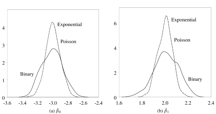
To demonstrate that the exponential, poisson, and binary-censored poisson models estimate the same effect parameters from the duration, count, and binary-censored data, respectively, we conducted a Monte Carlo analysis, letting the arrival rateλvary with a country-level covariate, orλ = exp(β0 +β1Xc). The true values of the effect parameters were set to
β0 = −3 andβ1=2.
A total of 200 simulations was run to obtain distributions of the estimated effects pa-rameters. Each simulation consisted of two parts: generating the data and running the maximum-likelihood regressions using the above models. In generating the data, for each of 200 countries, Xc was randomly distributed N(1,0.5) and durations of governments generated by exponentially distributed random draws, givenλ, up to a total of 10 time units. Counts were obtained for each country and the durations of each country were divided into unit lengths and the counts censored to obtain the binary data. The duration, count, and binary data were saved to data sets and the regressions were run to obtain the estimated parameters ˆβ0and ˆβ1.
Figures 2a and b show the resulting distributions of the Monte Carlo runs. Figure 2a shows that the exponential, poisson, and binary-censored poisson models all have similar distributions for the estimate of the constant term ˆβ0—in fact, the distributions of the
ex-ponential and poisson estimates appear to be identical when there is only a country-level covariate. Note also that the distributions are approximately normally distributed and cen-tered around the true valueβ0= −3.
Figure 2b shows much the same thing with respect to ˆβ1. The exponential, poisson, and
binary-censored poisson models all have similar distributions for the estimate of the country-level covariate’s coefficient ˆβ1. Again, the distributions of the exponential and poisson
estimates appear to be identical when there is only a country-level covariate. Similarly the distributions are approximately normally distributed and centered around the true value β1 =2.
Finally, since the logit model is so commonly used in the analysis of binary data, we compare it to the binary-censored poisson model. Unfortunately, the effect parameters of
9This model, as far as we know, is new. However, King (1989, pp. 225–226) uses similar notation in developing
(a) ˆβ0 (b) ˆβ1
Fig. 2 Time-independent data: densities of ˆβ0and ˆβ1 from the Monte Carlo analysis. The figures
show the densities of ˆβ0and ˆβ1 from regressions using the (a) exponential duration model (dotted
line), (b) poisson model (dashed line), and (c) binary censored-poisson model (solid line). The true values areβ0= −3 andβ1=2. All three models yield similar, approximately normal, distributions
for the parameter estimates, centered around the true value. In fact, the exponential and poisson densities are identical.N =200 for each density.
the logit are not comparable to those of the binary-censored poisson or, by extension, to those of the duration or poisson models. However, we can compare the two models in their predictions that at least one event will occur.
To do this, we generated data as before, lettingλ=exp(−3+2Xc), and ran a binary-censored poisson regression and a logit regression. Using the estimates obtained from these, we then plotted for each model the predicted probability of at least one event occurring over a sample of the simulated data. Figure 3 shows that the logit model predicts nearly identically to the binary-censored poisson model.10 However, although political scientists
may obtain nearly correct estimates using a logit model, we nevertheless believe that it is more appropriate to use a model derived from first principles. Doing so forces us to think theoretically about the data generating process. It also allows us to relate the parameter estimates directly (substantively and quantitatively) to the duration and count models of the same underlying data generation process.
4 Analyzing Time-Dependent Renewal Processes
The poisson process of Section 3 is a particular type of renewal process. It assumes not only that the durations of governments are independent and identically distributed, conditional on the explanatory variables, but that they are distributed exponentially. That is, after taking into account the explanatory variables and all events that have occurred up to timet, the probability of a new transfer of power remains the same in every period—i.e., the hazard rate is constant. Not surprisingly, there is considerable reason to believe that conditional time independence is not a reasonable assumption in many cases (e.g., Box-Steffensmeier
10Comparing plots of the logit and hurdle probabilities, King notes that the models are, for the most part, similar,
[image:12.612.119.480.93.284.2]Fig. 3 Time-independent data (β0= −3,β1=2): probability of event occurrence for the
censored-poisson and logit models. The figure shows the predicted censored-censored-poisson and logit probabilities of an event occurring for a sample of six countries over 10 time subintervals in each country. Each country is denoted by the number on thexaxis, with its 10 time subintervals following. The probability of an event occurrence is calculated for each subinterval using the country-varying dataXcand the
censored-poisson and logit regression estimates obtained from the larger data set. The figure shows that for time-independent data, the logit model predicts similarly to the censored-poisson model. Note, however, that, unlike the censored-poisson estimates, the logit estimates will not be directly comparable to the exponential and poisson estimates.
and Jones 1997; Beck et al. 1998). For example, Bienen and van de Walle (1991) argue that the durability of world leaders seem to follow a declining hazard rate. If a leader makes it past the first few years, the probability of losing power actually declines with time. Perhaps leaders that are more skillful are still in power later on, or, perhaps, only those countries with a custom of long leadership durations have leaders in power after 5 or 6 years. Whatever the explanation, a model that allows for increasing or decreasing hazard rates is essential, a task to which we now turn.11
Ideally, we would like a duration distribution that not only incorporates an increasing, decreasing, or nonmonotonic hazard rate, but also contains the exponential distribution as a special case. There are actually a number of duration distributions from which one might choose—e.g., the gamma, weibull, and normal distributions to name a few. The
11It is important to note, however, that temporal dependence in data can occur for one of two reasons: unobserved
[image:13.612.123.480.82.365.2]purpose of this paper is not to identify one distribution that researchers should use over others—which should be problem-specific and guided by theory—but rather to show how a time-dependent renewal process can be modeled and how the same effect parameters may be estimated from duration, count, and disaggregated data. For guidance concerning which distribution to choose—or whether to use a parameteric vs nonparametric method—we refer the reader to the references cited in the Introduction.
4.1 Duration Data
Suppose we believed that the durations between transfers of power were a result of one or more “shocks” to the governments, as, for example, in the “coalition of minorities” hypothesis. That is, a leader offends someone in the coalition every so often, and the coalition falls when saykcoalition members have been offended. Or suppose that a government can withstand onlyk“scandals” before it falls. If we assume that the underlying shocks to the government are independent and exponentially distributed, then the total duration between transfers of power is gamma distributed.
As the above implies, the gamma and exponential distributions are closely related. A duration random variableYcgwhich is the sum ofkindependent exponentially distributed random variables (e.g., durations) with arrival rateλis gamma distributed with parameters λandk, whereλ >0 andk≥1. The gamma probability density is given by
f(ycg|λcg,k)= yk−1
cg
(k)λ
k
e−λycg (14)
Fork>1, the failure rate is time dependent—in fact, it is an increasing failure rate. It is straightforward to see that ifk=1, then the gamma distribution reduces to the exponential distribution and the assumption of time independence, making this assumption a testable hypothesis.
Under this model, the expected duration isE(Ycg)=k/λ. We again letλ=exp(βxcg) vary as a function of explanatory variables. To estimate this model, we assume that the duration of successive governments are independent. This enables us to form the likelihood by taking the product of the densities over the countries and governments:
L(λ,k|ycg)=
c
g yk−1
cg
(k)λ
k e−λycg
=
c
g ycgk−1
(k)e
(xcgβ)ke−exp(xcgβ)ycg (15)
Althoughkis usually considered an integer, the duration model allows for nonintegerkand for testing whether the process has a constant failure rate (k=1) or an increasing failure rate (k>1). However, it does not allow one to distinguish whether the failure rate is constant versus decreasing.
4.2 Count Data
In deriving the gamma count model, we are interested in the number of gamma-distributed events that occur within a country’s observation periodTc. Recall that a gamma-distributed random variable with parameter λ is equivalent to the sum ofk exponentially distribu-ted random variables with arrival rateλ. It simplifies matters if we consider the gamma events as sequences of independent poisson events: for everykth poisson event (e.g., offense against a coalition member or appearance of a government scandal), a gamma event occurs (e.g., transition of power). For example, assumingk =3, zero gamma events implies that zero, one, or two poisson events occurred. Therefore, when we ask, What is the probability of zero gamma events in periodTc (givenk = 3)? we can equivalently ask, What is the probability of zero, one, or two poisson events inTc? Letting fp(·) be the poisson density,
we would more generally write (see also Ross 1993, p. 340; Winkelmann 1995, p. 469).
fγc(yc|λ,k,Tc)= fp(yck|λ,Tc)+ · · · + fp[(yc+1)k−1|λ,Tc] =
(yc+1)k−1
i=yck
fp(i |λ,Tc)
=
(yc+1)k−1
i=yck
e−λTc(λTc)
i
i! (16)
For nonnegative integer a, we can write the complement of the incomplete gamma function as
Q(a,x)=
a−1
i=0
e−xx i i! =
(a,x)
(a) (17)
where (a)=0∞e−tta−1dtis the standard gamma function and (a,x)=∞
x e− tta−1dt.
Using the incomplete gamma function, Eq. (16) becomes
fγc(yc|λ,k,Tc)=Q[(y+1)k, λTc]−Q[yk, λTc] (18)
The fact that we can express the gamma count density in terms of the same parameters as the gamma (duration) density allows us to estimate the same parameters from the count data that we can from duration data (with the exception, of course, of government-level covariates). As with the duration model, we allowλto vary as an exponential function of explanatory variables xc. The likelihood function for the count model is constructed by taking the product of Eq. (18) over all countries:
L(β,k|yc)=
c
Q[(y+1)k, λTc]−Q[yk, λTc]
=
c
Q[(y+1)k,excβTc]−Q[yk,excβTc] (19)
4.3 Disaggregated Data
as in the duration and country-level “aggregate” count models. To do this, we must provide a model forycgtderived from the gamma model ofycgabove. However, where in Section 3 we derived a binary model, here we instead derive a refined count model—one that is disaggregated over a country’s time series. We refer to this model as thedisaggregated gamma countmodel.
Modeling the disaggregated count data deserve a special section because of the problems induced by aggregation—or, rather disaggregation—in time-dependent data. Recall that for the poisson model, the arrival rate remains constant over time slices of equal size, no matter where those slices are sampled from on the time line. In contrast, for time-dependent data, where the time slice starts (and ends) matters, because the failure rate will be larger later in the life of a government. This was actually not a problem for the count model of our previous section, since we looked at the number of government transfers that occurred in the period (0,Tc), implying that we knew when the start of the first renewal was and that we did not have to take into account the disaggregation effects of dividing the (0,Tc) period into some number of artificial time slices.
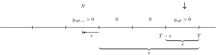
Before proceeding, we first define some additional notation, which corresponds to the time line in Fig. 4. LetT be the total time of a country up to the current observation,t
the duration of a government within that country up to the current observation, andsthe length of the time “slices.” We sometimes want to refer to time intervals in a more general way—i.e., allowing for time slicess=1—so letycg(t−s,t)be the number of gamma counts
in period (t−s,t) of governmentg for countryc. The number of events in time intervals starting att =0 can equivalently be written asycg(0,t)orycgt. However, we tend to use the
latter. Also, letN be the cumulative number of gamma counts for a country up to theprior
nonzero count relative to the current observation. Finally, letr be the unobserved length into the previous nonzero count interval, where the last gamma event actually occurred.
To derive the disaggregated gamma count distribution, we must account for two issues that arise due to the artificial divisions. First, we now have to deal with time slices that may exist in the “middle” of a government’s duration. Not only does the time dependence of the failure rate come into play here, but also we must condition on pastycgt. For example, if no gamma events occurs in two time periods and then ycg3gamma events occur in the
third period, then in calculatingycg3, we must condition on the fact that not enough poisson
events occurred during periods 1 and 2 to have caused a gamma event in either, but that there may have been poisson events in periods 1 and 2 which contributed to a gamma event in period three.
Fig. 4 Time line and notation for disaggregated gamma count model. The following notation is relative to the last period denoted by the down-arrow.tis the total time of a country up to the current observation.tis the duration of a government within that country up to the current observation.sis the length of the time “slices.”ycgt−1represents the last nonzero gamma count prior to the government
of the current observation.Nis the cumulative number of gamma counts for a country up to theprior
[image:16.612.125.475.529.619.2]The second issue is that in any period where one or more renewal occurs, we do not know where exactly the last renewal occurred in that period. Therefore, in calculating the probability ofycgtevents over some period of lengtht, we must average over the probabilities that the last renewal actually startedr back into the previous interval.
We leave the derivation of the disaggregated gamma count distribution for the Appendix and simply state it as
fd∗γc[ycg(t−s,t) |ycg(t−s) =0, λ,k]=
s
0
λe−λ(T−t−r)[λ(T−t−r)]
Nk−1
(Nk−1)!
Q[Nk, λ(T −t−s)]−Q[N k, λ(T −t)]
× k−1
i=0e−λ(
t−s+r)[λ(t−s+r)]
i
i! {Q[(ycgt+1)k−i, λs]−Q[ycgtk−i, λs]}
Q[k, λ(t−s+r)]
dr (20)
Note that all of the variables required to calculate fd∗γcare observable from the count data. Moreover, we now have an expression in the same terms as our duration and country-aggregated count model.
To form the likelihood, assume independence between gamma events having conditioned on the past, letλ=exp(xcβ), and take the product of the probabilities for each observation. In general, maximum-likelihood estimates forβandkwould be obtained by maximizing the log of the likelihood equation with respect toβ andk. However, one small problem remains. Traditional numerical search methods depend on continuous parameters. Here,
kcan only take on integer values since it is in the limit of the summation. We suggest a modified approach, where the user runs multiple maximum-likelihood regressions using Eq. (27) but holdsk constant at a different integer each time. The regression that yields the highest log-likelihood value determines the maximum-likelihood estimates of kand β. If, using this method, the maximum-likelihood estimate ofk is 1, then the user must examine whether the process is really time independent or if it actually has a decreasing failure rate—which would need to be modeled using a renewal model based on a different duration distribution.
4.4 An Example Using Simulated Time-Dependent Data
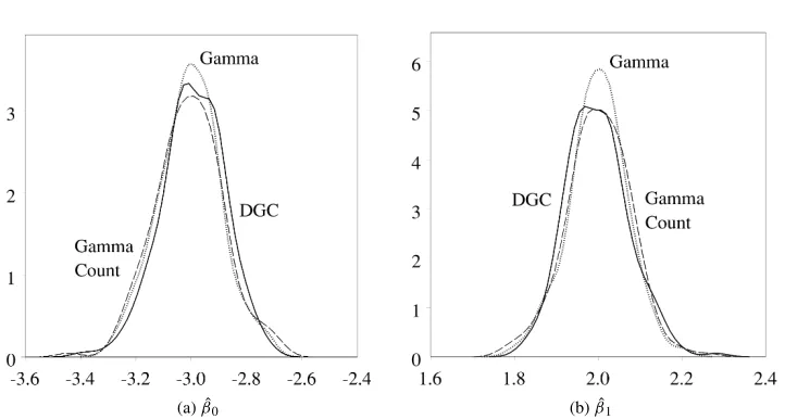
The log-likelihood equations for the gamma renewal models (especially the count models) are not trivial. In this section, we demonstrate (1) that the gamma, (country-aggregated) gamma count, and disaggregated gamma count models can actually be used to estimate effect parameters and (2) that they estimate the same effect parameters from the duration, count, and time-series disaggregated data, respectively. As in Section 3, we have conducted a Monte Carlo analysis, letting the arrival rate λvary with a country-level covariate, or λ=exp(β0+β1Xc). The true values of the parameters were set toβ0 = −3,β1=2, and
k=3. The basic procedure for simulating the data and running the regressions is identical to that outlined in Section 3, except that we generate gamma-distributed durations and the regressions use the gamma-based models just derived. Additionally, instead of unit length time periods for the binary model, we useds= 12.
(a) ˆβ0 (b) ˆβ1
Fig. 5 Time-dependent data: densities of ˆβ0and ˆβ1from Monte Carlo analysis. The figures show
the densities of ˆβ0 and ˆβ1 from regressions using the (a) gamma duration model (dotted line), (b)
aggregate gamma count model (dashed line), and (c) disaggregated gamma count model (solid line). All three models yield similar, approximately normal, distributions for ˆβ0and ˆβ, centered around the
true valuesβ0= −3 andβ1=2.N=200 for each density.
distributions are approximately normally distributed and centered around the true value β0= −3.
Figure 5b shows much the same thing with respect to ˆβ1. The gamma duration, gamma
count, and disaggregated gamma count models all have similar distributions for the estimate of the country-level covariate’s coefficient ˆβ1. The distributions are approximately normally
distributed and centered around the true valueβ1=2.
Finally, as in the time-independent case, we now compare the disaggregated gamma count model to commonly used specifications of logit. The analyst who believes that the data reflect some form of temporal dependence is unlikely to choose a time-independent logit model, like that in Section 3, where the probability of an event remains constant over time. An early suggestion of Beck (1998) is to use logit, but with time as a regressor,
y∗=β0+β1Xc+βtt+ (21)
wheret is operationalized as the duration up to the current observation. This allows the probability of an event occurrence to be an increasing or decreasing function of the time since the last event. We refer to this simply as “logit with time.” A specification recommended by Beck et al. (1998) is to include time dummies in the logit regression
y∗=β0+β1Xc+δ2D2+δ3D3+ · · · + (22)
Here, the dummies Dt are constructed for each of the discrete duration values realized in the data and then included as regressors in the logit model. This is a more flexible approach than “logit with time,” as it allows for the way in which time affects the probability of event occurrence to change over time. In general, however, it requires that many more parameters be estimated. We refer to this model as “logit with time dummies.”12
12Beck et al. (1998) propose that a cubic spline approach may be a better method than the time dummies, although
[image:18.612.120.481.91.284.2]Fig. 6 Time-dependent data (β0= −3,β1=2): probability of event occurrence for the disaggregated
gamma count and logit models. The graph shows the predicted disaggregated gamma count and logit probabilities of at least one event occurring for a sample of six countries over 20 time intervals in each country. Each country is denoted by the number on thexaxis, with its 20 time subintervals following. As the graph displays, both logit models do fairly well in capturing the temporal effects, although there are cases where they over-or underpredict by a wide margin.
As we noted in Section 3, the effect parameters of logit models are not comparable to those of the disaggregated gamma count model or, by extension, to those of the gamma or gamma count models. However, we can compare the logit and gamma models in their predictions that at least one event will occur. Following a similar procedure to the one outlined in Section 3.4, we assumedλ =exp(−3+2Xc) andk =3, generated data, ran disaggregated gamma count and logit regressions, and used the estimates to plot for each model the predicted probability of at least one event occurring over a sample of the simulated data. Figure 6 displays the predicted probabilities for each model for six countries over 20 time periods ofs= 12.
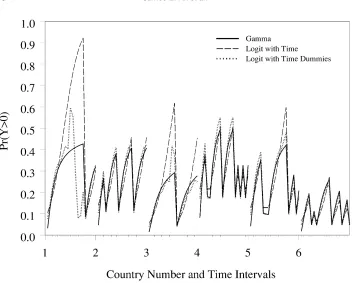
[image:19.612.124.478.87.370.2]Fig. 7 Extent to which logit will diverge from the gamma process. The graph displays the predicted probabilities for the disaggregated gamma count (solid line), logit with time (dashed line), and logit with time dummies (dotted line) models. As the graph shows, the logit models do not always predict the probabilities accurately. In general, they err the most in predicting large durations when Xcis
small. Logit with time dummies errs less than logit with time.
climbing in probability, the probability of government failure suddenly falls.13 A natural
question raised by this concerns when we should expect the logit with time and logit with time dummies models to diverge from the gamma data generating process.
To examine this question, we used Monte Carlo simulations (based on the data generation process described above) to estimate the average values of the parameter estimates in the logit with time and in the logit with time dummies models.14 For each of these, we then
plotted the gamma and logit probabilities of at least one event occurring. Figure 7 displays the predicted probabilities. Four hypothetical governments are shown, and each of the governments has 20 time intervals. The governments differ only in the values ofXc.
In general, Fig. 7 indicates (1) that both the logit with time and the logit with time dummies models are better at predicting shorter durations rather than longer durations and
13Beck et al. (1998) note that accurate estimation of the dummies requires a large sample size. In the Monte Carlo
analysis here, the sample size wasN=4000. Most political scientists would consider this a fairly large sample. Unfortunately, the literature is not yet clear on just how large a sample is needed for accurate dummy estimation.
14For the logit with time model,N = 1200 iterations resulted in mean parameter estimates of ˆβ
0 = −9.73,
ˆ
β1 =4.38, and ˆβt =.63, where ˆβt is the coefficient associated with the time regressor. For the logit with time dummies model,N=700 iterations resulted in mean parameter estimates of ˆβ0= −10.27, ˆβ1 =4.69,
ˆ
δ2 = .83, ˆδ3 = 1.22, ˆδ4 = 1.48, ˆδ5 = 1.65, ˆδ6 = 1.79, ˆδ7 =1.94, ˆδ8 = 1.97, ˆδ9 = 2.07, ˆδ10 = 1.98,
ˆ
δ11=1.93, ˆδ12=1.92, ˆδ13=2.18, ˆδ14=2.33, ˆδ15=2.59, ˆδ16=2.84, ˆδ17=2.53, ˆδ18=4.81, ˆδ19=4.41,
[image:20.612.122.478.97.369.2](2) that the logit with time dummies model is closer to the gamma than is logit with time. For example, note in the first government (Xc=1.5) that logit with time dummies is very close to the gamma model in periods 15 and 16, but logit with time errs by almost 0.6. However, in the last few periods, logit with time dummies errs by almost as much. The difference between the logit with time and the logit with time dummies models is not quite as stark for the other values ofXc.
The implications of these results are somewhat mixed concerning the recommendations of Beck (1998) and Beck et al. (1998). On the one hand, the results could be viewed as lending some theoretical support for these methods. By “theoretical support” we mean that including the time regressor or dummies produces predicted probabilities that are often fairly close in practice to those of the model that was derived from first principles and consistent with the data generating process. Because of the simplicity of these methods, they are obviously very attractive options. However, practitioners should understand that the predicted probabilities are not always accurate—and, in fact, can diverge greatly from the true probabilities. In particular, researchers should be careful in their predictions about longer durations. Whether our data provide enough information to distinguish between the models is of course another issue that needs further study in any real application.
Finally, although the logit with time and time dummies methods may be simple tools for addressing temporal dependence in practice, they were not designed to avoid aggregation bias. To do that, we need to understand the implications of a data generating process on different codings of the data. Only once we have a set of consistent models can we assess the impact of inappropriately aggregating data or of making incorrect assumptions in our analysis of aggregate data.
5 Concluding Remarks
We have derived models of binary, duration, and count data to represent identical underlying data generation processes—one requiring conditional independence among the events and one more general that allows a form of dependence. This analysis should help to show researchers the connections among the models applied to these various types of data. It should free them from the constraints the particular form of the data puts on their choice of models, encourage them to focus on the theory of what generated the data, and allow them to derive statistical models that are both consistent with the theory and appropriate for the data at hand. In doing so, we believe that this will facilitate comparisons of results across studies as the data is updated and perhaps changes formats.
We encourage future researchers to work out other consistent models of data at these, or other, levels of aggregation. This task will certainly be difficult at times. We have made a number of simplifications in this paper and, even with those, the resulting time-dependent disaggregated count model was not trivial to derive.
methods to weaken the present assumptions regarding independence of the parameters and regressors; this is particularly true since the dependence will usually also occur across the (often artificial) grouping categories. Fourth, the whole process of deriving consistent models forces us to pay more attention to our theories of what generated the data. If we political scientists are essentially studying the choices of individuals, then we need to think about the renewal processes that are consistent with individuals making choices. As Signorino (1999) and Signorino and Yilmaz (2000) show, failure to do so will guarantee misspecification and incorrect inferences.
These are but a few areas of the research agenda that stem directly from this paper. Other types of models will add even further complications. For example, Londregan and Poole (1990) use a simultaneous probit model to analyze binary data, Bienen and van de Walle (1991) use a proportional hazards model to study leadership duration, and Diermeier and Stevenson (1999) study these data with competing risks approaches. Further work needs to be done to determine precisely how these models aggregate so that they can be estimated from different forms of data and, especially, so that they can be compared with other studies which use these different forms of data. Finally, we hope that this agenda will eventually include results that help us understand and avoid aggregation bias as well.
Appendix: Disaggregated Gamma Count Model
To derive the disaggregated gamma count distribution fd∗γc, we start by addressing the issue of time dependence, ignoring for the moment any problems related to the issue of where the renewal process actually restarted. If the interval we are examining is preceded by an interval in which a gamma event occurs, then there is no problem of dependence between the current interval and the past lifetime of the government, since there is no additional past to the life of the government beyond the unobservablerinto the previous period, which is the subject of the second issue. However, if we are examining the second or higher period into the lifetime of a government, then the probability of a gamma event occurring in the current period is conditional on the poisson events that may have occurred in the previous periods for that government. Ignoring where the renewal process restarted, the disaggregated gamma count distribution is
fdγc[ycg(t−s,t) |ycg(t−s) =0]=
fdγc[ycg(t−s) =0,ycg(t−s,t)]
fdγc[ycg(t−s)=0]
(23)
where we have dropped the conditional notation forλandkfor the time being. Since the period for fdγc[ycg(t−s)] is (0,t−s), we can calculate this using Eq. (18).
To derive fdγc[ycg(t−s) = 0,ycg(t−s,t)], we again frame it in terms of the underlying
poisson events. For example, assumek=3 and letfp(y1,y2) be the joint poisson probability
thaty1poisson events occur in (0,t−s) andy2events occur in (t−s,t). Then
fdγc[ycg(t−s)=0,ycg(t−s,t)=0]
= fp(0,0)+ fp(0,1)+ fp(0,2)+ fp(1,0)+ fp(1,1)+ fp(2,0)
and
fdγc[ycg(t−s) =0,ycg(t−s,t)=1]
Generalizing (and recognizing that the joint poisson probabilities can be written as the product of their marginals), we get
fdγc[ycg(t−s)=0,ycg(t−s,t)]
= k−1
i=0
(ycg(t−s,t)+1)k−i−1
j=ycg(t−s)k−i
e−λ(t−s)[λ(t−s)] i i! e
−λs(λs)j
j! (24)
Substituting this and the appropriate form of Eq. (18) into Eq. (23) yields
fdγc[ycg(t−s,t)|ycg(t−s) =0, λ,k]
= k−1
i=0
(ycg(t−s,t)+1)k−i−1
j=ycg(t−s)k−i e
−λ(t−s)[λ(t−s)]
i i! e
−λs(λs) j j! k−1
i=0e−λ(t−s)
[λ(t−s)]i i!
= k−1
i=0e−λ(
t−s)[λ(t−s)]
i
i! {Q[(ycg(t−s)+1)k−i, λs]−Q[ycg(t−s)k−i, λs]}
Q[k, λ(t−s)] (25)
Equation (25) assumes that we can observe the start of a renewal and, therefore, specify it ast =0. However, when the durations (or country-aggregated counts) are divided into intervals, we often cannot observe where a renewal starts within an interval in which a gamma event occurs. Fortunately, we have probabilistic information about where the renewals start. What we want to know is the conditional probability that the renewal startedr back into the last nonzero gamma count period. If we letSNkbe the sum of the exponential durations from the country’s start to the previous nonzero count period, then the probability that the renewal startsrinto the previous nonzero count period, conditional on the fact that we know that the current renewal started in that period, is given by
f[SNk=T−t−r|T −t−s≤SNk≤T −t]
= f[SNk=T −t−r,T −t−s≤ SNk≤T −t] f[T −t−s≤ SNk≤T −t]
= f[SNk=T −t−r] f[T −t−s≤ SNk≤T −t]
= fγ[T −t−r|λ,Nk]
Fγ[T −t |λ,Nk]−Fγ[T −t−s|λ,Nk] (26) where fγ(t |λ,k) andFγ(t|λ,k) are the pdf and cdf of the gamma distribution.
To obtain the full distribution, we take the conditional probability Eq. (25), where we assume that the renewal start time is known and “average” it over the range of probable start times from Eq. (26), or
fd∗γc[ycg(t−s,t)|ycg(t−s)=0, λ,k]
=
s
0
f[SNk=T−t−r |T−t−s≤SNk≤T−t]
=
s
0
fγ[T −t−r|λ,Nk]
Fγ[T −t |λ,Nk]−Fγ[T −t−s|λ,Nk]
×fdγc[ycg(T−s,T)| ycg(T−t−r,T−s)=0]dr
= s 0
λe−λ(T−t−r)[λ(T−t−r)]
Nk−1
(Nk−1)!
e−λ(T−t−s)Nk−1
i=0
[λ(T −t−s)]i
i! −e
−λ(T−t)Nk−1
i=0
[λ(T −t)]i i!
× k−1
i=0
(ycgt+1)k−i−1
j=ycgtk−i e
−λ(t−s+r)[λ(t−s+r)]
i
i! e
−λs(λs)j j! k−1
i=0e−λ(t−s+r)
[λ(t−s+r)]i i! dr = s 0
λe−λ(T−t−r)[λ(T −t−r)] Nk−1
(Nk−1)!
Q[Nk, λ(T −t−s)]−Q[N k, λ(T −t)]
× k−1
i=0e−λ(
t−s+r)[λ(t−s+r)]
i i!
Q(ycgt +1)k−i, λs−Qycgtk−i, λs Q[k, λ(t−s+r)]
dr (27) References
Aalen, Odd O. 1992. “Modelling Heterogeneity in Survival Analysis by the Compound Poisson Distribution.” Annals of Applied Probability2(4):951–972.
Allison, Paul. D. 1982. “Discrete-Time Methods for the Analysis of Event Histories.” InSociological Methodology 1982, ed. S. Leinhardt. San Francisco: Jossey–Bass, pp. 61–98.
Allison, Paul D. 1984.Event History Analysis: Regression for Longitudinal Event Data. Beverly Hills, CA: Sage. Alt, James E., and Gary King. 1994. “Transfers of Governmental Power: The Meaning of Time Dependence.”
Comparative Political Studies27(2):190–211.
Beck, Nathaniel. 1998. “Modeling Space and Time: The Event History Approach.” InResearch Strategies in the Social Sciences, eds. Elinor Scarbrough and Eric Tanenbaum. Oxford: Oxford University Press. pp. 192–212. Beck, Nathaniel, Jonathan N. Katz, and Richard Tucker. 1998. “Taking Time Seriously: Time-Series-Cross-Section
Analysis with a Binary Dependent Variable.”American Journal of Political Science42(4):1260–1288. Bennett, D. Scott. 1997. “Testing Alternative Models of Alliance Duration, 1816–1984.”American Journal of
Political Science41(3):846–878.
Bennett, D. Scott, and Allan C. Stam III. 1996. “The Duration of Interstate Wars, 1816–1985.”American Political Science Review90(2):239–257.
Bienen, Henry, and Nicolas van de Walle. 1991. “Time and Power in Africa.”American Political Science Review 83:19–34.
Box-Steffensmeier, Janet M., and Bradford S. Jones. 1997. “Time Is of the Essence: Event History Models in Political Science.”American Journal of Political Science41(4):1414–1461.
Cameron, A. Colin, and Pravin K. Trivedi. 1998.Regression Analysis of Count Data. Cambridge: Cambridge University Press.