Possible binary progenitors for the Type Ib supernova iPTF13bvn
J. J. Eldridge,
1‹Morgan Fraser,
2Justyn R. Maund
3,4and Stephen J. Smartt
31Department of Physics, University of Auckland, Private Bag 92019, Auckland, New Zealand 2Institute of Astronomy, University of Cambridge, Madingley Road, Cambridge CB3 0HA, UK
3Astrophysics Research Center, School of Mathematics and Physics, Queen’s University Belfast, Belfast BT7 1NN, UK 4Department of Physics & Astronomy, University of Sheffield, Hicks Building, Hounsfield Road, Sheffield S3 7RH, UK
Accepted 2014 October 17. Received 2014 October 5; in original form 2014 August 18
A B S T R A C T
Cao et al. reported a possible progenitor detection for the Type Ib supernovae iPTF13bvn for the first time. We find that the progenitor is in fact brighter than the magnitudes previously reported by approximately 0.7–0.2 mag with a larger error in the bluer filters. We compare our new magnitudes to our large set of binary evolution models and find that many binary models with initial masses in the range of 10–20 Mmatch this new photometry and other constraints suggested from analysing the supernova. In addition, these lower mass stars retain more helium at the end of the model evolution indicating that they are likely to be observed as Type Ib supernovae rather than their more massive, Wolf–Rayet counter parts. We are able to rule out typical Wolf–Rayet models as the progenitor because their ejecta masses are too high and they do not fit the observed SED unless they have a massive companion which is the observed source at the supernova location. Therefore only late-time observations of the location will truly confirm if the progenitor was a helium giant and not a Wolf–Rayet star.
Key words: stars: evolution – binaries: general – supernovae: general – supernovae: individ-ual: iPTF13bvn.
1 I N T R O D U C T I O N
Massive stars end their lives in the explosive death throes of a core-collapse supernova (SN). These SNe are classified according to their observed spectra and light curves; in the first instance by the presence or absence of hydrogen in the SN spectrum – hydrogen-rich SNe are classified as ‘Type II’, while hydrogen-deficient SNe are ‘Type I’. Type I SNe are further divided1into Types Ib and Ic (collectively termed Type Ibc), which are helium rich and helium poor, respectively. While the progenitors of Type II SNe have been directly identified in pre-explosion images as H-rich supergiants between 8 and 16 M(Smartt et al.2009, and references therein), the progenitors of Type Ibc SNe have remained elusive.
The two likely candidates for the progenitors of Type Ibc SNe are single, massive Wolf–Rayet (WR) stars (Gaskell et al.1986), or lower mass stars in binaries (Podsiadlowski, Joss & Hsu1992). In both cases, the progenitor will be stripped of its H and/or He envelope. Eldridge et al. (2013) presented a sample of nearby Type Ibc SNe with pre-explosionHubble Space Telescope(HST) imag-ing, but found no progenitor candidates. Eldridge et al. suggested that this was evidence that a number of the progenitors of these
E-mail:[email protected]
1We note that Type Ia SNe are hydrogen-deficient SN from a thermonuclear
explosion mechanism in a carbon–oxygen white dwarf which we do not consider here.
SNe must been the result of an interacting binary star, as previously suggested from the relative rates of different SN types (De Donder & Vanbeveren 1998; Eldridge, Izzard & Tout2008; Smith et al.
2011). There is also growing additional evidence from statistical samples of ejecta masses that most Ib/c SNe are from low-mass stars in binaries (Drout et al.2011; Lyman et al.2014; Bianco et al.,
2014).
Last year Cao et al. (2013) presented the detection of a possi-ble progenitor candidate inHSTimages for the Type Ib supernova iPTF13bvn in the nearby galaxy NGC 5806. From the magnitudes they report for the progenitor candidate, along with indirect con-straints on its radius and mass-loss rate from observations of the SN itself, they suggested the progenitor of iPTF13bvn was consistent with a single WR star. Groh, Georgy & Ekstr¨om (2013) compared their single-star models to the constraints and found a possible initial mass range between 31 and 35 Mfor the progenitor. However, follow-up observations of iPTF13bvn yielded a bolometric light curve which, when fitted with a hydrodynamic model for the SN ejecta, implied a pre-explosion mass of∼3.5 M(Bersten et al.
In this paper, we first reanalyse the pre-explosion images of the site of the SN. We use late-timeHSTimages to revisit the astrometry and photometry of the progenitor candidate. We then compare the derived observational constraints for the progenitor of iPTF13bvn to our grid of binary evolution models from theBPASS(Binary Pop-ulation and Spectral Synthesis, http://bpass.auckland.ac.nz) code. While Bersten et al. (2014) have presented a binary progenitor sce-nario for iPTF13bvn, they note that their solution is not unique. Furthermore, we find the photometry of Cao et al. (2013) to which Bersten et al. (2014) fit their models to underestimates the progeni-tor candidates magnitudes. With our grid of models, we can compare a wide range of binary systems to the progenitor of iPTF13bvn, and constrain the allowed parameter space of the system.
In the following, we adopt a distance of 22.5±2.4 Mpc,µ=31.76
±0.36 mag towards NGC 5806, as used by Cao et al. and Fremling et al. from Tully et al. (2009). While the foreground reddening towards NGC 5806 is low (E(B−V)=0.045) from the Schlafly & Finkbeiner (2011) dust maps, the host galaxy reddenings adopted by Bersten et al., Cao et al. and Fremling et al. differ significantly. Bersten et al. find,E(B−V)=0.17±0.03, under the assumption that the colour evolution of iPTF13bvn matches that of other Type Ibc SNe; however, Cao et al. adopt a much lower value ofE(B−V)
= 0.03, from the strength of the Na D lines in high-resolution spectra. In this paper, we consider both possible values and find progenitors systems that fit between these two extinctions to take account of the uncertainty in the amount of dust.
2 O N T H E P R O G E N I T O R D E T E C T I O N
Cao et al. (2013) identified a progenitor candidate for iPTF13bvn in pre-explosionHST Advanced Camera for Surveys (ACS) im-ages, acquired as part of programme GO-10187 (PI: Smartt). These observations were acquired with the Wide Field Channel (WFC; pixel scale 0.05 arcsec pix−1) of ACS on 2005 March 10 using the
F435W(1600 s),F555W(1400 s) andF814W(1700 s) filters. A key outstanding question in the Cao et al. analysis, however, was the level of agreement between the position of the progenitor can-didate on the pre-explosion image and the transformed SN position derived from post-explosion adaptive optics images. Fremling et al. (2014) presented a re-analysis of the position of iPTF13bvn using
HST+WFC3 observations of iPTF13bvn, and found the Cao et al. progenitor candidate to be coincident with the SN. Using the same data as Fremling et al., we have performed an independent analysis of the position of iPTF13bvn.
NewHSTWide Field Camera 3 (WFC3; pixel scale 0.04 arcsec pix−1) Ultraviolet and Visual (UVIS) imager observations (F555W 1200 s) were taken of iPTF13bvn on 2013 September 2 (programme GO-12888, PI Van Dyk). Using theASTRODRIZZLEtask within the DRIZZLEPAC package, the under sampled WFC3_flt images were drizzled (Fruchter & Hook2002) on to a finer pixel scale, yield-ing a distortion corrected combined image with a pixel scale of 0.025 arcsec. The pre-explosion ACS images were taken at the same pointing, and so drizzling could not be used to improve their spatial resolution. However, the two individual_flc frames were still combined withASTRODRIZZLE(although with an output pixel scale of 0.05 arcsec) to remove cosmic rays and correct for the geometric distortion of ACS.
Using 29 point sources identified in both the ACSF555Wand WFC3 frames, we derived a geometric transformation between the pre- and post-explosion images with an rms error of 0.38 ACS pixels (19 mas). The pixel coordinates of iPTF13bvn were then measured on the post-explosion WFC3 image (as the SN is bright,
the uncertainty on its position is negligible in all of the following) and transformed to the ACS frame. We find the progenitor candidate of Cao et al. (2013) to be offset by only 7 mas from the transformed position of iPTF13bvn, and hence formally coincident, as also found by Fremling et al. (2014).
A caveat to this result, is that to correct the geometric distor-tion in the pre-explosion ACS image, we must resample the pixels in the image. We found through trials that the offset between the transformed SN position and the position of the progenitor can-didate was highly sensitive to the choice of parameters (e.g. the subtraction of the sky background, the shape of the kernel etc.) when correcting for this distortion using theASTRODRIZZLEandMUL -TIDRIZZLEpackages. We note that this effect was not observed for brighter nearby stars, and appeared to arise solely due to the relative faintness of the candidate. In comparison with bright nearby sur-rounding stars, we found the position of the progenitor candidate could change by as much as∼1.5 pixels, due to the way in which flux associated with the candidate was allocated into the pixels in its locality.
We hence performed a second alignment between the pre- and post-explosions, under the hypothesis that the_crj image was the least biased realization of the detected progenitor flux. We calcu-lated the geometric transformation between the distortedF555W _crj image (j90n02021_crj.fits) and the undistorted post-explosion WFC3F555Wimage, drizzled to 0.025 arcsec pix−1. To account for the distortion in the ACS frame, a fourth-order polynomial was used for the transformation, which had an rms error of 8 mas. The coordinates of iPTF13bvn were then transformed to the_crj image, where it lies at pixel coordinates 2698.09,593.38. The position of the progenitor candidate was measured using both theIRAF PHOT package and withDOLPHOT(Dolphin2000) to lie at 2698.0,593.83 and 2697.84,593.61 respectively. The progenitor candidate posi-tions fromPHOTandDOLPHOTare offset from the transformed SN position by0.5 pixels (25 mas); however, they are also offset from each other by 14 mas.
We performed point spread function (PSF)-fitting photometry of the pre-explosion_crj images using theDOLPHOTpackage (Dolphin
2000)2with the ACS module. Bad pixels were masked using the data quality images, beforeDOLPHOTwas run with the recommended parameters for ACS/WFC data. The progenitor candidate was de-tected in all three of the ACS filters. Interestingly, ifDOLPHOTis run on each of the filters separately, the magnitudes returned for the progenitor candidate are∼0.2 mag fainter than if all three filter images were input toDOLPHOTtogether. We measure magnitudes on individual images in the VEGAMAG system ofF435W=25.81± 0.06,F555W=25.86±0.08, F814W=25.77±0.10.
To check the output ofDOLPHOT, we also performed photometry on the pre-explosion images usingDAOPHOTwithinIRAF. Photometry was performed on the_drc files at the native ACS/WFC pixel scale of 0.05 arcsec pix−1. The_drc images have been corrected for both the inherent geometric distortion of ACS, and for losses due to CTE. For each filter, a PSF was constructed from bright, isolated point sources. The modelled PSF was then fitted simultaneously to both the progenitor candidate and all surrounding sources which may contribute flux at the position of the SN. The fit was made within a small (2 pixel) radius centred on each source, and the measured fluxes within this aperture were corrected to an infinite aperture using the tabulated corrections in Sirianni et al. (2005). Finally, the flux was converted to a magnitude in theHSTVEGAMAG system using the value of PHOTFLAM from the image header, and the flux of Vega in the corresponding filter from the HST webpages.3 We find magnitudes ofF435W=25.79±0.10,F555W=25.73± 0.07,F814W=25.99±0.22 for the progenitor candidate, which agree favourably with the results ofDOLPHOT. Because there is no clear reason to favour one over the other we use a mean of the two values. This gives magnitudes for the progenitor ofF435W=25.80
±0.12,F555W=25.80±0.11,F814W=25.88±0.24. Cao et al. (2013) reported magnitudes for the progenitor of
F435W=26.50±0.15,F555W= 26.40±0.15 andF814W=
26.10±0.20. It is not clear why there is such a great difference be-tween the two analyses. Other groups have also found magnitudes that agree with those we derive (van Dyk, private communication). We can only suggest, in light of the fact we obtain different results usingDOLPHOTandDAOPHOT, that the results are dependent on the parameters given to these codes when the photometry is derived and that any small error may be amplified.
The residual images after subtraction of the fitted PSFs were ex-amined, and do not show any gross over- or undersubtractions at the SN position. However, it is clear that the background is not smooth at the SN position, and late time observations after the SN has faded will be important to refine the progenitor candidate photometry using template subtraction (Maund, Reilly & Mattila2014).
3 N U M E R I C A L M E T H O D
The construction of the stellar models used in this paper have been described in detail in Eldridge et al. (2008). Here, we use these models and compare them to the progenitor candidate in a similar method to as in Eldridge et al. (2013), but now compare the models to an actual detection rather than upper limits on progenitor magni-tude. In summary, the stellar models follow single and binary stars at two metallicities,Z=0.008 and 0.020, that are close to the metallic-ity inferred for NGC 5806 of 12+log [O/H]=8.5 from Smartt et al.
2http://americano.dolphinsim.com/dolphot/
3http://www.stsci.edu/hst/acs/analysis/zeropoints/
(2009). In the models, the primary effect of metallicity is to vary the mass-loss rates via stellar winds. The evolutionary models are then matched to WR atmosphere models from the Potsdam group (e.g. Sander, Hamann & Todt2012) to enable their magnitudes to be calculated, as discussed in Eldridge & Stanway (2009). The grid of models covers initial masses of the primary from 5 to 120 M with mass ratios,m2/m1between 0.1 and 0.9 and initial separations in log (a/R) from 1.0 to 4.0.
The major difference in our method here to that of Eldridge et al. (2013) is that our aim is to demonstrate that single-star WR models are not the only possible progenitor and interacting binaries can fit the observed source and fit the other constraints available. Therefore, we compare the detected source to the end points of our models rather than considering the whole evolutionary track closer to the time of core-collapse. The latter is a more apt method to use when attempting to estimate accurate parameters for the progenitor and take into consideration uncertainties in the stellar evolution models themselves. But until post-explosion images are available to more tightly constrain the progenitor magnitudes, we consider only the final model end points. These are typically after the end of core-carbon burning and only a few years before core-collapse.
We have searched through our grid of models for stars which would give rise to a hydrogen-free SN and compared the magni-tude of these models to the magnimagni-tude derived in Section 2. With our assumed distance, the absolute magnitudes for the progenitor candidate areF435W= −5.96± 0.38,F555W= −5.97±0.38 andF814W= −5.88±0.43. We correct these magnitudes with the Bersten et al. (2014) and Fremling et al. (2014) extinction values to obtain our final magnitudes of between−6.15 and−6.67,−6.10 and
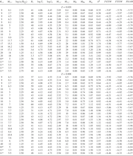
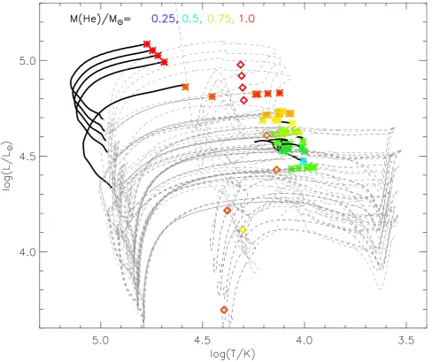
−6.49, and−5.95 and−6.13 for the progenitor candidate. These comparisons were made in theHSTfilter system to avoid the addi-tional uncertainty from converting to theUBVRIsystem. The upper limit of possible magnitudes are taken from magnitudes calculated with the higher extinction value and the lower bound is from the lower extinction value. We list the set of progenitor models which match the observed magnitudes of the progenitor candidate within the error bars, and within the range allowed by the uncertainty in extinction, in Table1. The evolutionary tracks of these models are plotted on a Hertzsprung–Russell diagram in Fig. 1, along with their spectral energy distributions (SED) compared to the observed magnitudes in Fig.2. In most cases, the SED is dominated by the primary, apart from in the few cases where the final mass of the secondary star is similar to the primary star’s initial mass. We cau-tion however, that the effect of mass transfer can cause dramatic evolutionary changes in the secondary star and much of the relevant physics is uncertain, as discussed by Claeys et al. (2011).
4 R E S U LT S
The large number of possible progenitor models means we need to consider also the secondary constraints from Cao et al. (2013), Fremling et al. (2014) and Bersten et al. (2014). We consider the constraint on the mass-loss rate, ejecta mass and the requirement for sufficient helium to produce a Type Ib SN. We do not use the radius constraint, because as pointed out by Bersten et al., this constraint is not as firm as first thought.
The constraint on the mass-loss rate from Cao et al. (2013) needs to be considered with care. Cao et al. assume a wind velocity of 1000 km s−1 to derive a mass-loss rate of approxi-mately 3 ×10⁻⁵M
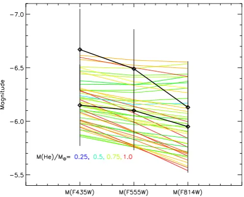
Table 1. Physical parameters of the binary progenitor models which match the observed constraints on the progenitor of iPTF13bvn. Models where the primary mass has an asterisk beside it are systems with a compact objects for a secondary; the secondary masses of 0.6, 1.4 or 2.0 Mcorrespond to a white dwarf, neutron star or black hole, respectively. The given magnitudes are for the combined system of primary and secondary together. All systems however are dominated by the emission from the primary star. All masses, radii and luminosities are in given in units of M, Rand L, respectively. Surface temperatures are given in kelvin.
M1,i M2,i log (a/R) R1 logT1 logL1 M1,f M2,f MH MHe Mej A F435W F555W F814W
Z=0.020
9 8.1 2.25 41 4.06 4.43 2.05 8.4 0.00 0.66 0.60 0.35 −5.87 −5.78 −5.72
9 2.7 2.50 48 4.03 4.44 2.07 2.7 0.00 0.67 0.62 0.38 −6.03 −5.97 −5.95
9 4.5 2.50 59 3.99 4.44 2.08 4.6 0.00 0.68 0.63 0.41 −6.22 −6.19 −6.21
9 6.3 2.50 65 3.97 4.44 2.09 6.5 0.00 0.68 0.64 0.43 −6.29 −6.27 −6.31
9 8.1 2.50 69 3.95 4.44 2.09 8.4 0.00 0.68 0.64 0.44 −6.29 −6.29 −6.38
10 5 2.25 40 4.10 4.55 2.29 5.1 0.00 0.64 0.83 0.65 −6.00 −5.89 −5.79
10 7 2.25 43 4.08 4.56 2.30 7.2 0.00 0.65 0.84 0.69 −6.10 −5.99 −5.90
10 9 2.25 45 4.07 4.56 2.31 9.3 0.00 0.66 0.87 0.71 −6.15 −6.05 −5.98
10 5 2.50 63 4.01 4.58 2.36 5.1 0.00 0.69 0.92 0.88 −6.47 −6.43 −6.44
11 9.9 2.75 29 4.21 4.69 2.82 10 0.00 0.84 1.37 0.87 −5.95 −5.78 −5.58
13 11.7 1.25 61 4.00 4.52 2.19 22 0.00 0.60 0.74 0.71 −6.38 −6.34 −6.36
17 15.3 1.50 4.4 4.69 4.99 4.21 26 0.00 1.01 2.70 1.74 −5.98 −5.77 −5.54
18 16.2 1.50 4.0 4.72 5.03 4.45 28 0.00 1.03 2.98 2.03 −6.11 −5.91 −5.67
19 17.1 1.50 3.6 4.75 5.05 4.65 29 0.00 1.02 3.20 2.30 −6.20 −5.99 −5.76
20 14 1.25 6.1 4.58 4.86 3.50 29 0.00 0.94 2.02 0.99 −6.01 −5.83 −5.64
20 18 1.50 3.3 4.77 5.08 4.91 30 0.00 1.01 3.41 2.82 −6.29 −6.08 −5.84
10* 5 2.25 56 4.01 4.47 2.06 2.2 0.00 0.42 0.62 0.56 −6.24 −6.16 −6.17
11* 3.3 2.50 38 4.15 4.69 2.75 1.4 0.00 0.82 1.27 1.07 −6.07 −5.91 −5.79
11* 5.5 2.50 55 4.06 4.67 2.74 2.0 0.00 0.81 1.29 1.15 −6.50 −6.37 −6.31
11* 3.3 2.75 41 4.13 4.69 2.81 1.4 0.00 0.83 1.35 1.05 −6.18 −6.01 −5.90
11* 5.5 2.75 40 4.13 4.69 2.80 2.0 0.00 0.83 1.35 1.05 −6.16 −6.00 −5.88
Z=0.008
9 6.3 2.25 37 4.11 4.53 2.14 6.5 0.00 0.60 0.69 0.58 −5.92 −5.83 −5.76
9 8.1 2.25 39 4.10 4.53 2.14 8.4 0.00 0.60 0.70 0.59 −5.98 −5.90 −5.84
9 2.7 2.50 43 4.08 4.53 2.16 2.7 0.00 0.62 0.72 0.64 −6.11 −6.05 −6.02
9 6.3 2.50 59 4.01 4.54 2.19 6.5 0.00 0.63 0.75 0.76 −6.35 −6.34 −6.42
10 3 2.25 34 4.15 4.61 2.49 3.0 0.00 0.72 1.02 0.72 −5.87 −5.76 −5.66
10 5 2.25 40 4.12 4.62 2.51 5.1 0.00 0.74 1.06 0.81 −6.11 −6.02 −5.94
10 7 2.25 43 4.10 4.62 2.52 7.1 0.00 0.74 1.07 0.83 −6.21 −6.13 −6.07
10 9 2.25 45 4.09 4.62 2.52 9.3 0.00 0.74 1.07 0.85 −6.26 −6.19 −6.15
10 3 2.50 54 4.05 4.62 2.55 3.0 0.00 0.75 1.10 0.92 −6.44 −6.41 −6.42
10 7 2.50 60 4.03 4.63 2.58 7.2 0.01 0.77 1.12 0.92 −6.51 −6.49 −6.54
11 9.9 1.25 35 4.13 4.57 2.29 18 0.00 0.67 0.84 0.63 −5.86 −5.76 −5.67
11 7.7 2.25 31 4.19 4.71 2.93 7.8 0.01 0.86 1.48 0.98 −5.92 −5.77 −5.61
11 9.9 2.25 33 4.18 4.72 2.93 10 0.01 0.86 1.49 1.01 −5.99 −5.85 −5.70
11 3.3 2.50 43 4.12 4.72 2.96 3.3 0.01 0.87 1.48 1.16 −6.30 −6.20 −6.12
11 5.5 2.50 54 4.08 4.72 2.97 5.5 0.01 0.87 1.53 1.30 −6.58 −6.52 −6.49
11 7.7 2.50 56 4.07 4.72 2.98 7.8 0.01 0.88 1.50 1.32 −6.62 −6.57 −6.55
12 8.4 1.25 41 4.11 4.62 2.49 18 0.00 0.72 1.05 0.82 −6.14 −6.05 −5.98
12 10.8 1.25 42 4.11 4.63 2.56 20 0.00 0.76 1.10 0.82 −6.18 −6.09 −6.02
12 8.4 2.50 29 4.24 4.82 3.38 8.5 0.01 0.96 1.93 1.83 −5.94 −5.76 −5.57
12 10.8 2.50 30 4.23 4.82 3.39 11 0.01 0.97 1.94 1.90 −6.08 −5.90 −5.71
12 3.6 2.75 38 4.18 4.83 3.42 3.6 0.01 0.97 1.96 2.17 −6.28 −6.14 −6.00
12 6 2.75 49 4.12 4.83 3.44 6.0 0.02 0.98 1.94 2.57 −6.60 −6.50 −6.42
40 12 1.25 11 4.45 4.81 3.31 42 0.01 0.94 1.87 1.00 −6.01 −5.86 −5.69
10* 5 2.50 43 4.10 4.63 2.54 2.1 0.00 0.73 1.10 0.89 −6.23 −6.10 −6.04
11* 3.3 2.50 43 4.13 4.73 2.95 1.4 0.01 0.84 1.50 1.33 −6.31 −6.17 −6.09
11* 5.5 2.50 48 4.11 4.73 2.94 2.0 0.01 0.84 1.50 1.43 −6.46 −6.33 −6.27
wind speeds evolve towards the end of a star’s evolution and vary with final mass. Therefore, a more reliable constraint is to consider the wind density, which is dependent on fewer as-sumptions. We use the dimensionless wind parameter,A∗, where
A∗=( ˙M/10−5Myr−1)/(vwind/1000 km s−1). Therefore, values of the order unity are similar to those from the typical WR star. From Cao et al., iPTF13bvn has a value ofA∗=3 therefore some-what dense compared to the typical WR wind. The mass-loss rate
Figure 1. HR diagram showing the evolutionary tracks for models which match the constraints on the progenitor candidate of iPTF13bvn. The tracks are for two metallicities withZ=0.008 and 0.020. Thin grey dashed lines – evolution tracks with hydrogen, thick black lines – evolution without hydrogen. Asterisks – end point of progenitor models, diamonds – location of secondary star at explosion, they are included to indicate the general locations possible for the secondary star. Colour indicates helium mass in the primary at the end point of the model.
a range between 0.4 and 3. The measured value is dependent on other physical assumptions so we do not regard this as a significant disagreement.
The ejecta mass derived by Fremling et al. (2014) for iPTF1bvn is around 1.94+0.50
−0.58M. This should be considered a lower limit as there may always be additional helium that is transparent and unobservable as described by Piro & Morozova (2014). We estimate an ejecta mass for our models by calculating the binding energy of the star and using this to estimate how much mass would be ejected if 1051erg of energy was injected into the envelope as described in Eldridge & Tout (2004). Only in cases where the binding energy of the stellar envelope is higher than this would there be material left to fall back on to the central protoneutron star. As our models have an initial mass less than 20 M, we find that a neutron star is always produced so the ejecta mass is effectively the final mass minus 1.4 M. For each model, a corresponding minimum observed ejecta mass can be estimated by subtracting the amount of helium in the stellar model from the ejecta mass quotes in Table1. We constrain our model selection again by requiring the ejecta mass
to be less than 3.5 M. This upper limit is estimated by using the upper limit from the error in the ejecta mass and up to 1 Mof helium being transparent (Piro & Morozova2014). We find that our model ejecta masses are in reasonable agreement with the value of Fremling et al. (2014), typically lying between 1 and 2 M.
The minimum amount of helium which a star must retain to the point of core-collapse if it is to produce the spectroscopic signature of a Type Ib SN is still somewhat uncertain (Dessart et al.2011). In nearly all our models, there is greater than 0.5 Mof helium in the ejecta, likely to be enough to provide the required Type Ib SN spectrum. We note that in some of the models there is a small amount of hydrogen left on the surface of the star at the end of our models. Because our models end at the end of carbon burning it is possible that this hydrogen would subsequently be removed, in addition the mass-loss rates of such stars are highest, and least certain at the end of their lives, when they become helium giants.
Figure 2. SED of progenitor models compared to limits derived here with both the low and high extinction values used. The error bars on the observed limits are mainly determined by the error in the distance to the host galaxy. Here the colours of the lines represent the helium abundance of the model as for the points in Fig.1. Most of the models are relatively cool with shallow or flat SEDs.
survived by a visible, albeit faint, stellar companion. There is also a subset of systems where the companion will be a compact object, and undetectable at optical wavelengths. We do not predict the mag-nitude for the secondary companion, as the parameters of this star will be strongly affected by the mass transfer process. Finally, we note that we do find that some very massive stars with initial masses of 80 Mdo match our magnitude range. However these have very low amounts of helium, large ejecta masses of around 5–7 Mand the SED is dominated by the binary companion. In this case, the observed SED therefore represents the binary companion not the progenitor itself.
5 D I S C U S S I O N A N D C AV E AT S
In contrast to the conclusion of Groh et al. (2013), we cannot find any single-star models which match the SED of the progenitor can-didate for iPTF13bvn. This is largely due to our revised magnitudes being brighter than previously reported, especially with the brighter
F435Wmagnitude. In addition to the other constraints such as the total mass and mass of helium ejected, we note that our single-star models do not include rotation so our analysis does not rule out a single-star solution completely. Therefore similar to Bersten et al. (2014), we conclude that iPTF13bvn most likely did not come from a non-rotating single-star progenitor.
We caution that current uncertainties in stellar models could weaken this result. For example the role of envelope inflation of WR stars, an increase in their radius due to radiation pressure on the iron-opacity peak, is still the subject of research and debate. Therefore, the single-star radii could be smaller or greater than ex-pected from models. In addition mass-loss rates of WR stars are still to some extent uncertain so models may lose less mass during the WR phrase and therefore contain more helium when they explode. From our models, we favour a binary progenitor for iPTF13bvn, most likely a low-mass helium giant in a binary system. While such a helium giant would have a radius larger that the limit of<5 R derived by Cao et al. (2013). Bersten et al. (2014) have suggested that for this SNe, as for SN 2011dh (Bersten et al.2012), detailed
modelling demonstrates that the initial constraints on the progenitor radius are not as stringent as first suggested.
We stress that all binary models represent a ‘best-guess’ as to the evolution of massive interacting binary stars. The largest uncer-tainty remains the contribution from the binary companion of the progenitor to the SED of the progenitor system. As discussed by Stancliffe & Eldridge (2009) and Claeys et al. (2011), the evolu-tion of these stars post-mass-transfer is uncertain, and they may be cooler than normally expected for a main-sequence star. Detection of any surviving companion in late-time imaging of the SN site will provide an important constraint on the binary scenario. Furthermore a spectrum of the star may reveal that it is rapidly rotating because of the binary interactions (De Mink et al.2013).
6 C O N C L U S I O N S
We have presented revised magnitudes for the source that is coinci-dent with the SN iPTF13bvn. TheF435Wis the most significantly brighter by 0.7 mag. This changes the shape of the source SED and therefore has a strong influence on the resulting possible objects that can match the progenitor source.
Using these new magnitudes and allowing for a range of extinc-tions measured by different methods, we find that it is possible to match the source and other secondary constraints with binary mod-els that had initial masses between 10 and 20 M. This overlaps with the model suggested by Bersten et al. (2014).
More massive models tend to not fit the source SED without a bright companion star. Therefore if the source still exists when the SN fades then the progenitor was a more massive WR star rather than a lower mass helium giant. However, we suggest that the latter is highly favoured in light of the ejecta mass estimates of Bersten et al. (2014) and Fremling et al. (2014). This is also in agreement with the prediction that helium giants would be easier to identify as the progenitor of a Type Ib/c SN by Yoon et al. (2012).
It is only with late-time imaging that a deeper insight will be gained into the progenitor. This has been demonstrated by analysis of even the relatively well understood progenitors of Type IIP SNe (Maund et al.2014). If a surviving companion star is found at the site of iPTF13bvn, then for the first time the binary evolution of a Type Ib SN progenitor can be studied in detail.
AC K N OW L E D G E M E N T S
JJE acknowledges support from the University of Auckland. This work was partly supported by the European Union FP7 pro-gramme through ERC grant number 320360. SJS acknowledge funding from the European Research Council under the European Union’s Seventh Framework Programme (FP7/2007-2013)/ERC Grant agreement no. [291222] and STFC grants ST/I001123/1 and ST/L000709/1. The research of JRM is supported by a Royal Soci-ety Research Fellowship.
R E F E R E N C E S
Bersten M. C. et al., 2012, ApJ, 757, 31 Bersten M. C. et al., 2014, ApJ, 148, 68 Bianco F. B. et al., 2014, ApJS, 213, 19 Cao Y. et al., 2013, ApJ, 775, L7
Claeys J. S. W., de Mink S. E., Pols O. R., Eldridge J. J., Baes M., 2011, A&A, 528, A131
de Mink S. E., Langer N., Izzard R. G., Sana H., de Koter A., 2013, ApJ, 764, 166
Dessart L., Hillier D. J., Livne E., Yoon S.-C., Woosley S., Waldman R., Langer N., 2011, MNRAS, 414, 2985
Dolphin A. E., 2000, PASP, 112, 1383 Drout M. R. et al., 2011, ApJ, 741, 97
Eldridge J. J., Stanway E. R., 2009, MNRAS, 400, 1019 Eldridge J. J., Tout C. A., 2004, MNRAS, 353, 87
Eldridge J. J., Genet F., Daigne F., Mochkovitch R., 2006, MNRAS, 367, 186
Eldridge J. J., Izzard R. G., Tout C. A., 2008, MNRAS, 384, 1109 Eldridge J. J., Fraser M., Smartt S. J., Maund J. R., Crockett R. M., 2013,
MNRAS, 436, 774
Fremling C. et al., 2014, A&A, 565, A114 Fruchter A. S., Hook R. N., 2002, PASP, 114, 144
Gaskell C. M., Cappellaro E., Dinerstein H. L., Garnett D. R., Harkness R. P., Wheeler J. C., 1986, ApJ, 306, L77
Groh J. H., Georgy C., Ekstr¨om S., 2013, A&A, 558, L1
Lyman J., Bersier D., Phil J., Paolo M., Eldridge J., Fraser M., Elena P., 2014, MNRAS, submitted
Maund J. R., Reilly E., Mattila S., 2014, MNRAS, 438, 938 Nugis T., Lamers H. J. G. L. M., 2000, A&A, 360, 227 Podsiadlowski P., Joss P. C., Hsu J. J. L., 1992, ApJ, 391, 246 Prio A. L., Morozova V. S., 2014, ApJ, 792, L11
Sander A., Hamann W.-R., Todt H., 2012, A&A, 540, A144 Schlafly E. F., Finkbeiner D. P., 2011, ApJ, 737, 103 Sirianni M. et al., 2005, PASP, 117, 1049
Smartt S. J., Eldridge J. J., Crockett R. M., Maund J. R., 2009, MNRAS, 395, 1409
Smith N., Li W., Filippenko A. V., Chornock R., 2011, MNRAS, 412, 1522 Stancliffe R. J., Eldridge J. J., 2009, MNRAS, 396, 1699
Tully R. B., Rizzi L., Shaya E. J., Courtois H. M., Makarov D. I., Jacobs B. A., 2009, AJ, 138, 323
Yoon S.-C., Grfener G., Vink J. S. Kozyreva A., Izzard R. G., 2012, A&A, 544, 11